A Data-Driven Fault Diagnosis Method for Solid Oxide Fuel Cell Systems

Abstract

In this study, a data-driven fault diagnosis method was developed for solid oxide fuel cell (SOFC) systems. First, the complete experimental data was obtained following the design of the SOFC system experiments. Then, principal component analysis (PCA) was performed to reduce the dimensionality of the obtained experimental data. Finally, the fault diagnosis algorithms were designed by support vector machine (SVM) and BP neural network to identify and prevent the reformer carbon deposition and heat exchanger rupture faults, respectively. The research results show that both SVM and BP fault diagnosis algorithms can achieve online fault identification. The PCA + SVM algorithm was compared with the SVM algorithm, BP algorithm, and PCA + BP algorithm, and the results show that the PCA + SVM algorithm is superior in terms of running time and accuracy, the diagnosis accuracy reached more than 99%, and the running time was within 20 s. The corresponding system optimization scheme is also proposed.

1. Introduction

A fuel cell is an energy conversion device that converts the chemical energy of fuel directly into electrical energy, which has the advantage of high efficiency without creating pollution or noise [1]. A solid oxide fuel cell (SOFC) operating at high temperature has a wider range of advantages compared to other fuel cells [2]. First, SOFCs offer fuel flexibility: SOFCs operate at high temperatures from 550 to 1000 °C, and therefore support internal reforming of gaseous hydrocarbon fuels. This means SOFCs are highly flexible in fuel selection and tolerant of a certain level of common fossil fuel impurities, such as ammonia, chlorides, and compounds containing sulfur [3]. Second, the high quality waste heat from SOFCs is suitable for cogeneration applications: the electrical efficiency of a stand-alone SOFC system is about 55%, and the energy conversion efficiency can be further increased to more than 85% by combining the cogeneration method to recycle the waste heat to generate additional electricity [4]. Third, SOFCs have lower costs, resulting in greater profitability: the high temperature operation eliminates the need for precious metal catalysts for SOFCs, resulting in lower costs and resulting in greater profitability [5]. Therefore, compared with other fuel cells, SOFCs have the advantages of high efficiency, wide fuel applicability, high waste heat quality, and relatively low cost. They also have a wide range of application scenarios, with power levels ranging from W-class to MW-class, mainly involving portable power generation, transportation, distributed power generation, and stationary power generation [6].

As SOFC systems become less tolerant of decreasing reliability and safety, their fault diagnosis is becoming an integral part of SOFC control systems and consists of three main tasks: (1) detection—detecting the presence of undesired states in the system [7]; (2) isolation—locating or classifying different faults; and (3) analysis or identification—determining the type, size, or possible cause of the fault [8]. Peng et al. [9] conducted a detailed review and analysis of SOFC system fault diagnosis research, pointing out the shortcomings of existing methods, and noting future research directions.

In the past decade, a large number of studies on SOFC system status monitoring and fault diagnosis have emerged, which can be broadly summarized into two categories in terms of approach [10,11,12]: model based and data based.

One approach is the model-based fault diagnosis scheme, which starts by building a model of the SOFC system with predetermined values of several physicochemical variables that represent the behavior of the system in a healthy state. Then, during system operation, the predetermined values of these variables are compared with the actual values to obtain residual values (i.e., indicators of deviation between measured and predetermined values). Since the model and the real system receive the same inputs and the model simulates the health of the system, when the real system is fault free, the residuals are zero, and are less than the thresholds for model uncertainty and the measurement tolerance. Conversely, when a fault occurs, the residuals will be larger than a certain threshold [13]. Murshed et al. [14] proposed a monitoring method that describes the fault detection problem as a linear matrix inequality. The method was used in a real SOFC system to detect early faults. Polverino et al. [15,16,17] studied SOFC field fault diagnosis algorithms and developed a dynamic model for simulating SOFC systems under fault conditions. The scheme compares the fault model with the normal SOFC system to determine if a fault has occurred and to infer the actual fault type with the help of a Fault Signature Matrix (FSM). However, this method is not used for online fault diagnosis because the model is too complex and requires a long processing time. Gallo et al. [18] defined health and fault states using a SOFC system component model and used FSM for fault monitoring and identification. Based on this, a fault mitigation strategy was developed to extend the lifetime. However, this solution can only identify typical faults with known principles; if the faults are not typical, they must be re-modeled, and therefore unknown faults cannot be detected. Wu et al. [19] developed a state observer for detecting flow sensor faults and fuel input actuator faults based on a thermal characteristic model. However, the observer can only work at pre-set operating points, and once the system deviates from the pre-set operating points, the observer cannot continue to detect faults. Xu et al. [20] developed a novel gas leak state estimator combined with a Kalman filter to diagnose SOFC gas leak faults, and compared the performance of different fault diagnosis strategies under different leak states. The results show that the proposed fault diagnosis strategy has good practicality and can guide compensation schemes for leaks.

The other approach is the data-based fault diagnosis scheme, which uses historical process data to measure the degree of interaction between process variables and then obtains the causal relationships between the variables. This scheme does not require mechanistic modeling, but rather extracts the underlying information from a large amount of historical data to show the dependence of system variables [21]. The data-based diagnostic scheme requires a sufficient training phase to enable it to distinguish between the healthy state of the system and each fault state. This scheme has two main implementations: supervised classifiers [22,23,24,25] and artificial neural networks [26,27,28]. Moser et al. [13] designed a support vector machine (SVM)-based fault diagnosis method for SOFC stack degradation, air leakage, fuel leakage, and reformer degradation faults; this method works well under different operating conditions and fault sizes. The diagnosis results show that the correct diagnosis rate of the scheme for the faults is higher than 80%. However, the four types of fault data used for SVM training are generated by the mechanism model, and the accuracy of fault diagnosis can also be affected if the mechanism model is not accurate enough. Li et al. [22] proposed a multi-label (ML) pattern recognition method to identify the simultaneous occurrence of multiple faults in SOFC systems. This method only requires the use of a dataset consisting of a single fault without requiring simultaneous fault data. Experimental results show that the proposed method is able to diagnose simultaneous SOFC system faults with high accuracy, and requires only a small amount of training data and has a low computational burden. However, during the training of the model, only some of the health and fault data were intercepted, and the most comprehensive system performance could not be obtained. Wu et al. [29] used a fault diagnosis scheme based on a square support vector machine (LS-SVM) classifier to diagnose anode poisoning and cathode moisture faults and to predict the remaining service life of SOFC systems. The results show that the LS-SVM model has a maximum fault identification rate of 97% and the prediction error of the remaining service life is within ±20%. Zhang et al. [30] established a general SOFC system fault diagnosis method based on deep learning (DL). Experimental results show that the accuracy of the proposed Deep Neural Network (DNN) method is very high, reaching more than 99%, both on small and large datasets. In the methods provided by Wu [29] and Zhang [30] et al., the data used also rely on model generation and are not directly obtained from system experiments, so the diagnostic results obtained are affected by the accuracy of the mechanistic model.

More studies on SOFC fault diagnosis can be found in the reviews of [7,9,12,31].

Both of these fault diagnosis schemes are currently inadequate and suffer from several problems:

• The model-based fault diagnosis scheme is used to determine whether the system is faulty by building a nonlinear physical model of the SOFC system. However, the model-based approach has some difficulties in ensuring model accuracy: (1) due to the existence of uncertain parameters and disturbances, the model must be simplified accordingly, which will lead to model uncertainty; (2) the SOFC system is a complex nonlinear model having a large number of coupling relationships in the system, and it is difficult for the model to accurately restore the performance of the system; and (3) the actual system becomes increasingly complex, and the model runs thus often require considerable processing time, which is not suitable for real-time diagnosis.
• In most of the studies of data-based fault diagnosis, the data used are generated by models. These studies face the same problems as those of the model-based schemes. The lack of accuracy in the data generated leads to the lack of accuracy in the diagnostic results obtained. The most accurate conclusions can only be obtained by using the data obtained during the operation of the actual system.
• In much of the literature that uses actual data for research, only a portion of the experimental data is intercepted for analysis, and the entire process of the experiment is not addressed. However, the SOFC system experimental data are a set of time series, and the most comprehensive system performance can be obtained only by analyzing the full phase data.

In order to improve the relevance and physical realizability of fault diagnosis methods, in this study, a data-driven fault diagnosis method for SOFC systems was constructed. It is divided into the following steps: (1) Conducting kW-level SOFC system experiments and analyzing experimental data under full working conditions. (2) Dimensionality reduction in experimental data using principal component analysis (PCA). PCA is an analysis technique that simplifies data, converting originally complex multidimensional data into simple, intuitive, and relevant low-dimensional data through dimensionality reduction, effectively reducing the difficulty and complexity of data analysis. Zhang et al. [32] proposed a fault diagnosis strategy combining PCA, simulated annealing genetic algorithm fuzzy c-means clustering (SAGAFCM), and a deep belief network (DBN) to diagnose faults occurring in fuel cell powered vehicles, in which PCA simplifies a large amount of data, and greatly optimizes the diagnosis results and improves the diagnosis speed. (3) The support vector machine (SVM) classifier and the BP neural network classifier are trained separately to obtain the fault diagnosis model, and the performance of the model is examined. The SVM and BP algorithms are the two most representative and easy-to-implement algorithms among supervised classifiers and artificial neural networks, respectively, so these two algorithms were chosen in the current study as the base models for comparison with Long Short-Term Memory (LSTM) and Recurrent Neural Network (RNN) algorithms. Xu et al. [33] proposed a fault diagnosis algorithm based on SVM to diagnose faults occurring in tracks and gearboxes, and the results showed that the diagnostic accuracy reached 96.7%; compared with other algorithms, SVM was superior in fault diagnosis, which is of great importance for industrial safety and reliability. Xiao et al. [34] also developed a fault diagnosis algorithm based on a BP neural network for faults in gearboxes, and also achieved an accuracy above 90%, illustrating the superiority of the BP algorithm.

The research solution proposed in this paper has the following main innovations: (1) For SOFC systems, this paper solves the problem of faults that are difficult to distinguish and diagnose, which is caused by the large amount of raw data and the complex system mechanism, and provides a new way of thinking for system performance optimization. (2) This scheme does not rely on complex system mechanism models, and only requires experimental data to locate, mark, and diagnose faults. It can be used not only for SOFC systems, but also for numerous systems where faults are difficult to diagnose directly, such as proton exchange membrane fuel cell systems, rolling bearing systems, and gearbox systems. (3) In this paper, the two most representative approaches in supervised classifiers and artificial neural networks are compared, reflecting the characteristics of each of the two schemes.

This paper is organized as follows: In Section 2, the structure of the SOFC system is described. In Section 3, the SVM-based fault diagnosis algorithm is introduced. In Section 4, the fault diagnosis scheme based on the BP neural network is presented. In Section 5, the proposed fault diagnosis scheme for SOFC systems is analyzed and discussed based on the obtained experimental results. The SVM and BP methods with and without PCA are also compared. Finally, conclusions are presented.

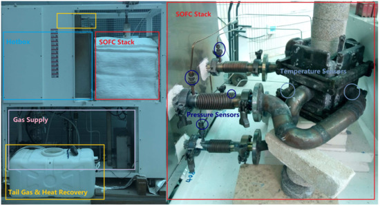
2. SOFC System Architecture

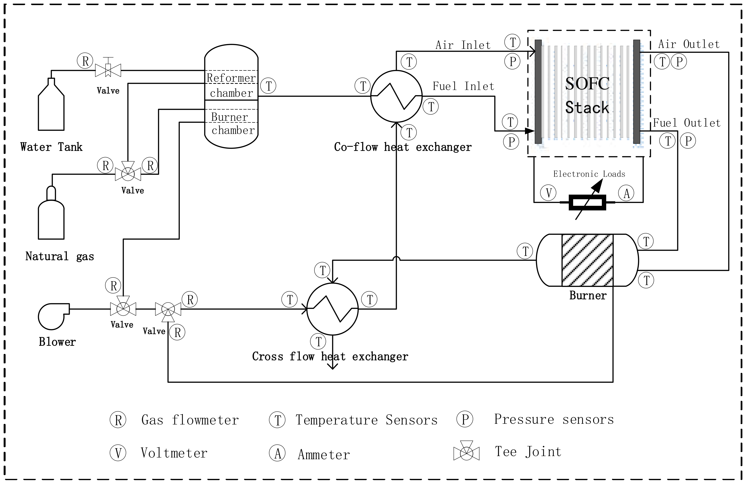
This experiment used a 1 kW SOFC system, whose main components include an SOFC stack, reformer, air–exhaust gas heat exchanger, fuel–air heat exchanger, exhaust gas combustion chamber, desulfurizer, dehumidifier, air compressor, air storage tank, electric lighter, cooling water tank, and monitoring system, as shown in Figure 1.

The reformer used in this system not only has combustion reactions of natural gas and air, but also high temperature reforming chemical reactions that produce CO and H₂. The combustion and reforming reactions take place in two separate chambers in the reformer. Electric firing triggers the combustion of natural gas and air, which provides high temperatures of approximately 600 to 700 °C to provide heat for the reforming reaction.

Inside the exhaust gas combustion chamber, the remaining fuel in the stack, which is not involved in the electrochemical reaction, is fully burned and its main function is to supply heat to the entire SOFC system. At the beginning of the system operation, it heats the stack to above 600 °C, thus enabling the discharge function of the stack. During system operation, it is mainly used to maintain the temperature balance in the SOFC system, while the excess heat it generates can be used for external cogeneration. To prevent tempering from causing temperature safety problems in SOFC stacks and pipes, the tail gas combustion chamber is filled with a porous medium.

The SOFC system studied in this paper contains two heat exchangers: an exhaust gas–air heat exchanger and a fuel–air heat exchanger, respectively. The two heat exchangers perform different functions. The function of the exhaust–air heat exchanger raises the temperature of the cathode air by exchanging heat between the high temperature exhaust gas coming from the exhaust combustion chamber and the cold cathode air that has just been introduced into the system. In this case, the temperature of the cathode air is raised to 500–700 °C after the first heat exchange. The function of the fuel–air heat exchanger is to exchange heat between the reformed high temperature fuel and the cathode air after the first heat exchange in order to reduce the temperature difference between the anode gas and the cathode air.

In addition to the above components, other auxiliary components—air flow meters, fuel flow meters, pumping pumps, desulfurizers, water evaporators, industrial control equipment, and electronic loads—are required to perform the functions of the SOFC system for power generation. The flow meter controls the amount of fuel and air entering the system; the pump passes cooling water and deionized water into the system; the desulfurizer desulfurizes the natural gas to prevent the sulfur in the fuel from poisoning the SOFC stack; the water evaporator vaporizes the liquid deionized water into water vapor; the industrial control equipment collects the signals returned through the various sensors installed on the SOFC system and sends real-time control signals; and the electronic load applies an external power demand and collects information, such as the current and voltage of the SOFC stack.

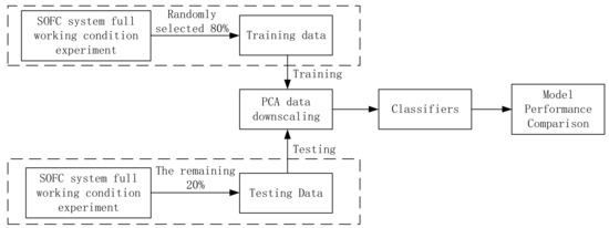
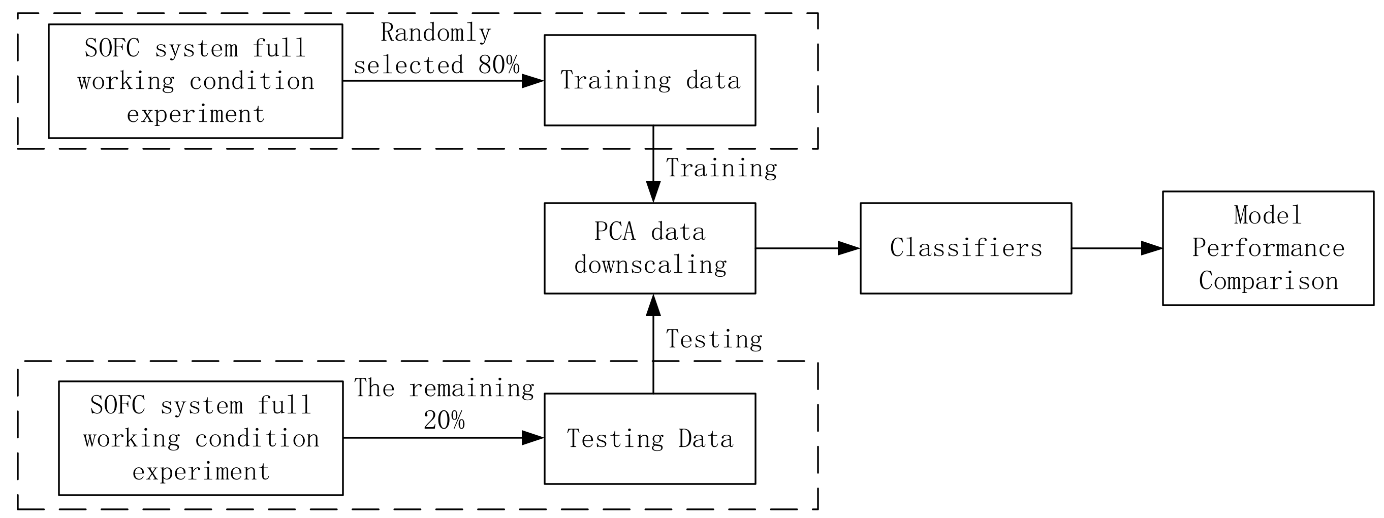
In order to diagnose the faults occurring in the SOFC system, in this study, an experiment using the SOFC system in full working condition was conducted to obtain the system data under actual operation conditions. A share of 80% of the data was randomly selected as the training data of the diagnostic model, and the remaining 20% of the data was used as the test data. Then, the obtained data were subjected to PCA data dimensionality reduction, retaining the low-order principal components and removing the high-order components to achieve the purpose of reducing the dimensionality of the dataset. Next, the dimensionality reduction data were used to train SVM, BP and other classifiers to obtain fault diagnosis models; finally, the test data were used to verify the accuracy of each diagnosis model and to compare them, as shown in Figure 2.

3. PCA-Based Data Dimensionality Reduction

In the real data collected, the data are usually affected by noise. In addition, when the dataset is large, it is likely to contain data triggered by exceptions. Low-quality data can affect the results of the fault diagnosis algorithm, so it is important to pre-process the data before training the model. The first step is to clean the data, fill in the missing values, smooth the noisy data, and identify and remove outliers. The data were then normalized to place all variable values between [0,1] to eliminate the effect of dimensional and numerical differences between different variables.

In the SOFC system experiments, 82 variables were collected by sensors in the cold and hot zones, and it is thus difficult for the fault diagnosis algorithm to quickly diagnose faults from the multidimensional information. Therefore, we need to first reduce the dimensionality of the data by a priori knowledge and principal component analysis (PCA), and then divide the reduced data into two parts, one for training the fault diagnosis model and one for verifying the accuracy of the model.

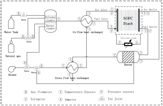
During the experiment, the PLC in the SOFC system recorded a total of 82 variables, namely, 21 variables in the cold box and 61 variables in the hot box, as shown in Figure 3.

In order to perform rapid diagnosis of faults, the data needs to be downscaled first. The first step is to perform a primary screening of the data by a priori knowledge. For example, eight Boolean state variables (ON/OFF status of valve units, system operating status, etc.) are removed because they have no impact on the training of the fault diagnosis model. After the initial screening, 10 variables were retained that were representative of the system performance: fuel input flow rate, fuel input flow rate to the combustion chamber, air input flow rate to the reformer, bypass air flow rate, deionized water input flow rate, reformer temperature, heat exchanger temperature, combustion chamber temperature, current, and voltage.

Principal component analysis (PCA) is then applied to the 10 variables for dimensionality reduction; PCA is an analysis technique that simplifies the data by transforming the problem from high to low dimensions through linear transformations, retaining low-order principal components and removing high-order components for the purpose of reducing the dimensionality of the dataset. The original complex multidimensional data are converted into simple, intuitive, and relevant low-dimensional data through dimensionality reduction, effectively reducing the difficulty and complexity of data analysis. The flow of PCA implementation is shown in Figure 4.

Assuming that after normalizing the original data, the resulting matrix is $D_{N\times m}=\left(x^{\left(1\right)},x^{\left(2\right)},\dots ,x^{\left(m\right)}\right)$:

(1)

Calculate the covariance matrix of the matrix D: $D{D}^T$.

(2)

Obtain the eigenvalue decomposition of the matrix $D{D}^T$.

(3)

Analyze the eigenvalues of the matrix $D{D}^T$, take out the eigenvectors $\left({\omega }_1,{\omega }_2,\dots ,{\omega }_{n^{\prime }}\right)$ corresponding to the largest n′ eigenvalues, and normalize them to form the eigenvector matrix W.

(4)

Transform each sample $x^{\left(i\right)}$ into a new sample $z^{\left(i\right)}=W^T{x}^{\left(i\right)}$.

(5)

Finally, the reduced dimensional dataset $D_{n^{\prime }\times m}^{\prime }=\left(z^{\left(1\right)},z^{\left(2\right)},\dots ,z^{\left(m\right)}\right)$ is obtained.

4. SVM-Based Fault Diagnosis Solution

To extend the life of a solid oxide fuel cell system and maximize the performance of the cell, it is important to develop a troubleshooting system that can detect and identify faults early. When a SOFC system fails, it can cause a significant degradation in system performance. Therefore, finding a fast fault detection method for SOFC systems is a prerequisite to ensure stable, efficient, and long-life operation. In this study, a support vector machine (SVM)-based fault diagnosis algorithm was designed, and the SVM model was trained and validated with the data obtained by dimensionality reduction in the previous section.

A support vector machine (SVM) is a supervised learning model that is commonly used to deal with binary classification problems. The multi-classification problem can also be implemented by training multiple binary classifiers. The method has good robustness, and therefore is widely used in many tasks and shows strong advantages.

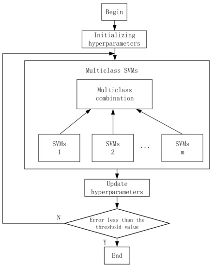
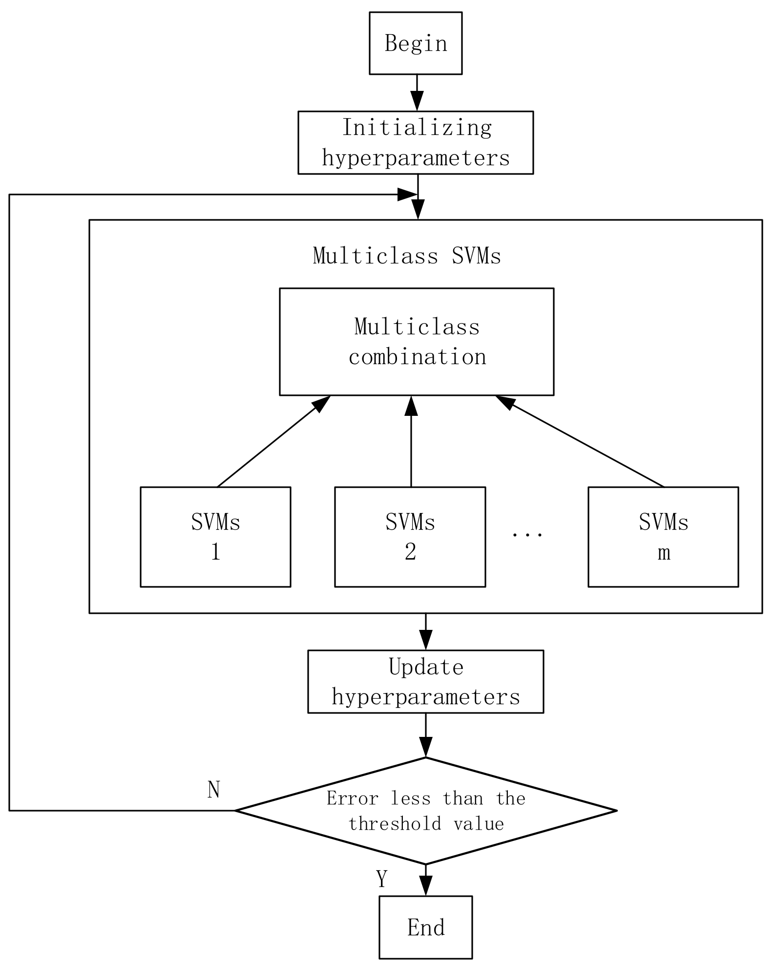
To implement the m classification problem using SVM, m two-class classifiers need to be trained. Classifier i is sets the label of the i-th class of data as class 1 (positive class), and the labels of all other m−1 classes other than class i are jointly set as class 2 (negative class), so that a two-class classifier needs to be trained for each class and, finally, we have a total of m classifiers. For data x that needs to be classified, the category with the highest confidence level is usually chosen to label the classification result. The flow chart of the implementation of the multiclassification SVM algorithm is shown in Figure 5.

The mechanism of SVM is to find an optimal classification hyperplane that satisfies the classification requirements such that the hyperplane can maximize the blank area on both sides of the hyperplane while ensuring the classification accuracy.

Suppose there is a binary dataset $R={\left\{\left(x^{\left(n\right)},y^{\left(n\right)}\right)\right\}}_{n=1}^N$ where $y_n\in \left\{+1,-1\right\}$. If the two classes of samples are linearly separable, then there exists a hyperplane ${\omega }^{T}x+b=0$, which separates the two classes of samples, and then each sample has $y^{\left(n\right)}\left({\omega }^T{x}^{\left(n\right)}+b\right)>0$.

The distance from each sample $x^{\left(n\right)}$ in the dataset R to the segmentation hyperplane is ${\gamma }^{\left(n\right)}=\frac{\left|{\omega }^T{x}^{\left(n\right)}+b\right|}{\left|\left|\omega \right|\right|}=\frac{y^{\left(n\right)}\left({\omega }^T{x}^{\left(n\right)}+b\right)}{\left|\left|\omega \right|\right|}$. Assume that $\gamma =\underset{n}{min}{\gamma }^{\left(n\right)}$ is the shortest distance from all samples in the entire dataset R to the segmentation hyperplane. A larger $\gamma$ means a more stable division of the two datasets and less susceptibility to noise. The goal of the SVM is to find a hyperplane $\left({\omega }^{*},b^{*}\right)$ such that $\gamma$ is the maximum:

$$\begin{gathered} \underset{\omega ,b}{max} \\ s.t.\frac{y^{\left(n\right)}\left({\omega }^T{x}^{\left(n\right)}+b\right)}{\left|\left|\omega \right|\right|}\ge \gamma , \forall n\in \left\{1,\dots ,\mathrm{N}\right\} \end{gathered}$$

(1)

Since simultaneous scaling of $\omega$ and b does not change the distance from the sample to the segmented hyperplane, here restricting $\left|\left|\omega \right|\right|\cdot \gamma =1$. For linearly divisible datasets, there are multiple segmentation hyperplanes, but the hyperplane with the largest interval is unique. SVM can solve nonlinear problems by mapping the original data to a higher dimensional space using kernel functions. The commonly used kernel functions are the linear kernel function, radial basis function (RBF), and polynomial kernel function. The RBF kernel function is usually used to deal with nonlinear differentiability problems. The RBF kernel function can be expressed by the following equation: $k\left(x,z\right)=\exp -\frac{|\left|x-z\right|{|}^2}{2{\sigma }^2}$. where σ is the width of the RBF.

In the optimization problem of support vector machines, the constraints are more stringent. If the samples in the training set are not linearly separable in the feature space, the optimal solution cannot be found. In order to be able to tolerate some of the samples that do not satisfy the constraints, slack variables can be introduced, transforming the optimization problem into:

$$\begin{gathered} \begin{array}{ll}& \underset{\omega ,b}{min} \frac{1}{2}|\left|\omega \right|{|}^2+C{{\displaystyle \sum }}_{n=1}^N{\xi }_n\\ & s.t.1-y^{\left(n\right)}\left({\omega }^T{x}^{\left(n\right)}+b\right)-{\xi }_n\le 0, \forall n\in \left\{1,\cdots ,N\right\}\end{array} \\ {\xi }_n\ge 0, \forall n\in \left\{1,\cdots ,N\right\} \end{gathered}$$

(2)

where ${\xi }_n$ is the relaxation factor and C is the penalty factor to control the balance of the interval and relaxation variables.

5. Fault Diagnosis Scheme Based on a BP Neural Network

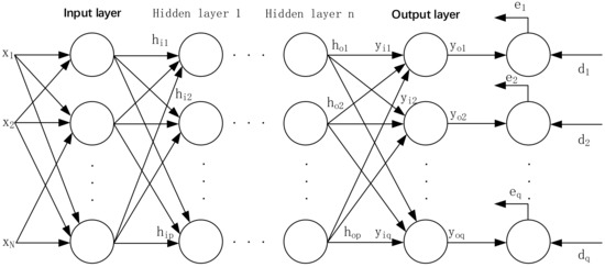
The BP neural network was proposed in 1986 by a group of scientists led by Rumelhart and McCelland as a multilayer feedforward network trained by an error backpropagation algorithm. The input data are gradually processed by the hidden layer until the output, and the parameters of each neuron and the threshold are adjusted backwards according to the output and the expected error, so that the output is closer and closer to the expected value. BP networks have become the most widely used artificial neural networks to date because of their excellent nonlinear mapping ability, generalization ability, and fault tolerance. The BP neural network is a variant of the perceptron and is highly capable of classifying and dividing nonlinearities. BP networks are supervised feed-forward networks, so the prediction of the network has to be trained first, and the associative memory and prediction ability are acquired through training, like in the human brain.

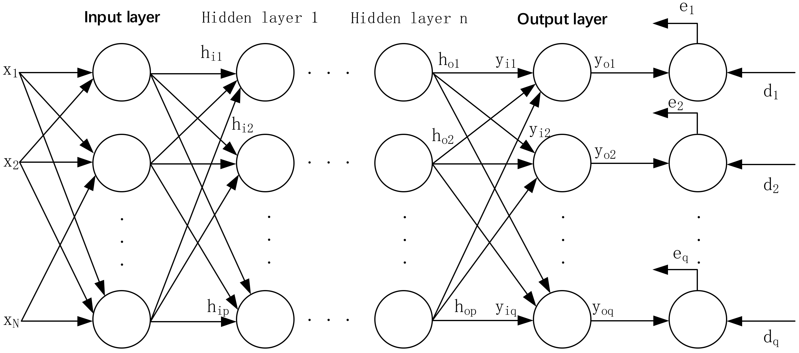
BP networks can learn and store a large number of input–output pattern mapping relationships without the need to describe the mathematical equations of such mapping relationships in advance. Its learning rule is to use the fastest descent method to continuously adjust the weights and thresholds of the network by back propagation to minimize the sum of the squared errors of the network. The topology of the BP neural network model includes an input layer, hidden layer, and output layer, as shown in Figure 6.

The main idea of BP neural network implementation is to input the learning samples, and then use the back propagation algorithm to iteratively adjust the weights and deviations of the network training, so that the output vector is as close as possible to the desired vector. The training is completed when the sum of squared errors of the output layer of the network is less than the specified error, and the weights and deviations of the network are saved, as shown in Table 1.

Table 1. Implementation process of a BP neural network.

1. Network initialization: assign a random number in the interval (−1,1) to the connection weights, set the error function$e$, and give the computational accuracy $\epsilon$ and the maximum learning number M.
2. Random selection: the kth output sample is randomly selected along with the corresponding expected output:
$x\left(k\right)=\left(x_1\left(k\right),x_2\left(k\right),\dots ,x_n\left(k\right)\right), d_o\left(k\right)=\left(d_1\left(k\right),d_2\left(k\right),\dots ,d_q\left(k\right)\right)$	(3)
3. Hidden layer computation: Compute the input and output of each neuron in the hidden layer, $h=1,2,\dots ,p$$, o=1,2,\dots ,q$:
$h_{ih}\left(k\right)={{\displaystyle \sum }}_{i=1}^n{w}_{ih}{x}_i\left(k\right)-b_h, h_{oh}\left(k\right)=f\left(h_{ih}\left(k\right)\right)$	(4)
$y_{io}\left(k\right)={{\displaystyle \sum }}_{h=1}^p{w}_{ho}{h}_{oh}\left(k\right)-b_o, y_{oo}\left(k\right)=f\left(y_{io}\left(k\right)\right)$	(5)
4. Find the partial derivative: Using the expected and actual outputs of the network, the partial derivative ${\delta }_o\left(k\right)$ of the error function is calculated for each neuron in the output layer.
5. Corrected weights: the connection weights ${\omega }_{ho}\left(k\right)$ are corrected using ${\delta }_h\left(k\right)$ of each neuron in the output layer and the output of each neuron in the hidden layer.
$\Delta {\omega }_{ho}\left(k\right)=-\mu \frac{\partial e}{\partial {\omega }_{ho}}=\mu {\delta }_o\left(k\right)h_{oh}\left(k\right), {\omega }_{ho}^{N+1}={\omega }_{ho}^N+\eta {\delta }_o\left(k\right)h_{oh}\left(k\right)$	(6)
6. Corrected weights: use the ${\delta }_o\left(k\right)$ of each neuron in the hidden layer and the input of each neuron in the input layer to correct the connection weights.
$\Delta {\omega }_{ih}\left(k\right)=-\mu \frac{\partial e}{\partial {\omega }_{ih}}={\delta }_h\left(k\right)x_i\left(k\right), {\omega }_{ih}^{N+1}={\omega }_{ih}^N+\eta {\delta }_h\left(k\right)x_i\left(k\right)$	(7)
7. Calculation of global error:
$E=\frac{1}{2m}{{\displaystyle \sum }}_{k=1}^m{{\displaystyle \sum }}_{o=1}^q{(d_o\left(k\right)-y_o\left(k\right))}^2$	(8)
8. Judging the reasonableness of the model: judge whether the network error meets the requirements, and end the algorithm when the error reaches the preset accuracy or the number of learning steps is larger than the designed maximum number. Otherwise, select the next learning sample and the corresponding output expectation, return to step 3, and enter the next round of learning.
Input variables: $x=\left(x_1,x_2,\dots ,x_n\right),$ hidden layer input variables: $h_i=\left(h_{i1},h_{i2},\dots ,h_{ip}\right),$ hidden layer output variables: $h_o=\left(h_{o1},h_{o2},\dots ,h_{op}\right),$ output layer input variables: $y_i=\left(y_{i1},y_{i2},\dots ,y_{iq}\right),$ output layer output variables: $y_o=\left(y_{o1},y_{o2},\dots ,y_{oq}\right),$ expected output vector: $d_o=\left(d_1,d_2,\dots ,d_q\right),$ connection weights of the input layer and the hidden layer: ${\omega }_{ih},$ connection weights of the hidden layer and the output layer: ${\omega }_{ho},$ threshold value of each neuron in the hidden layer: $b_h,$ threshold of each neuron in the output layer: $b_o,$ number of sample data: $k=1,2,\dots ,m,$ activation function: $f\left(•\right),$ error function: $e=\frac{1}{2}{{\displaystyle \sum }}_{o=1}^q{(d_o\left(k\right)-y_{oo}\left(k\right))}^2$.

Table 1. Implementation process of a BP neural network.

1. Network initialization: assign a random number in the interval (−1,1) to the connection weights, set the error function$e$, and give the computational accuracy $\epsilon$ and the maximum learning number M.
2. Random selection: the kth output sample is randomly selected along with the corresponding expected output:
$x\left(k\right)=\left(x_1\left(k\right),x_2\left(k\right),\dots ,x_n\left(k\right)\right), d_o\left(k\right)=\left(d_1\left(k\right),d_2\left(k\right),\dots ,d_q\left(k\right)\right)$	(3)
3. Hidden layer computation: Compute the input and output of each neuron in the hidden layer, $h=1,2,\dots ,p$$, o=1,2,\dots ,q$:
$h_{ih}\left(k\right)={{\displaystyle \sum }}_{i=1}^n{w}_{ih}{x}_i\left(k\right)-b_h, h_{oh}\left(k\right)=f\left(h_{ih}\left(k\right)\right)$	(4)
$y_{io}\left(k\right)={{\displaystyle \sum }}_{h=1}^p{w}_{ho}{h}_{oh}\left(k\right)-b_o, y_{oo}\left(k\right)=f\left(y_{io}\left(k\right)\right)$	(5)
4. Find the partial derivative: Using the expected and actual outputs of the network, the partial derivative ${\delta }_o\left(k\right)$ of the error function is calculated for each neuron in the output layer.
5. Corrected weights: the connection weights ${\omega }_{ho}\left(k\right)$ are corrected using ${\delta }_h\left(k\right)$ of each neuron in the output layer and the output of each neuron in the hidden layer.
$\Delta {\omega }_{ho}\left(k\right)=-\mu \frac{\partial e}{\partial {\omega }_{ho}}=\mu {\delta }_o\left(k\right)h_{oh}\left(k\right), {\omega }_{ho}^{N+1}={\omega }_{ho}^N+\eta {\delta }_o\left(k\right)h_{oh}\left(k\right)$	(6)
6. Corrected weights: use the ${\delta }_o\left(k\right)$ of each neuron in the hidden layer and the input of each neuron in the input layer to correct the connection weights.
$\Delta {\omega }_{ih}\left(k\right)=-\mu \frac{\partial e}{\partial {\omega }_{ih}}={\delta }_h\left(k\right)x_i\left(k\right), {\omega }_{ih}^{N+1}={\omega }_{ih}^N+\eta {\delta }_h\left(k\right)x_i\left(k\right)$	(7)
7. Calculation of global error:
$E=\frac{1}{2m}{{\displaystyle \sum }}_{k=1}^m{{\displaystyle \sum }}_{o=1}^q{(d_o\left(k\right)-y_o\left(k\right))}^2$	(8)
8. Judging the reasonableness of the model: judge whether the network error meets the requirements, and end the algorithm when the error reaches the preset accuracy or the number of learning steps is larger than the designed maximum number. Otherwise, select the next learning sample and the corresponding output expectation, return to step 3, and enter the next round of learning.
Input variables: $x=\left(x_1,x_2,\dots ,x_n\right),$ hidden layer input variables: $h_i=\left(h_{i1},h_{i2},\dots ,h_{ip}\right),$ hidden layer output variables: $h_o=\left(h_{o1},h_{o2},\dots ,h_{op}\right),$ output layer input variables: $y_i=\left(y_{i1},y_{i2},\dots ,y_{iq}\right),$ output layer output variables: $y_o=\left(y_{o1},y_{o2},\dots ,y_{oq}\right),$ expected output vector: $d_o=\left(d_1,d_2,\dots ,d_q\right),$ connection weights of the input layer and the hidden layer: ${\omega }_{ih},$ connection weights of the hidden layer and the output layer: ${\omega }_{ho},$ threshold value of each neuron in the hidden layer: $b_h,$ threshold of each neuron in the output layer: $b_o,$ number of sample data: $k=1,2,\dots ,m,$ activation function: $f\left(•\right),$ error function: $e=\frac{1}{2}{{\displaystyle \sum }}_{o=1}^q{(d_o\left(k\right)-y_{oo}\left(k\right))}^2$.

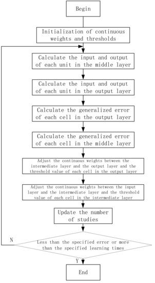
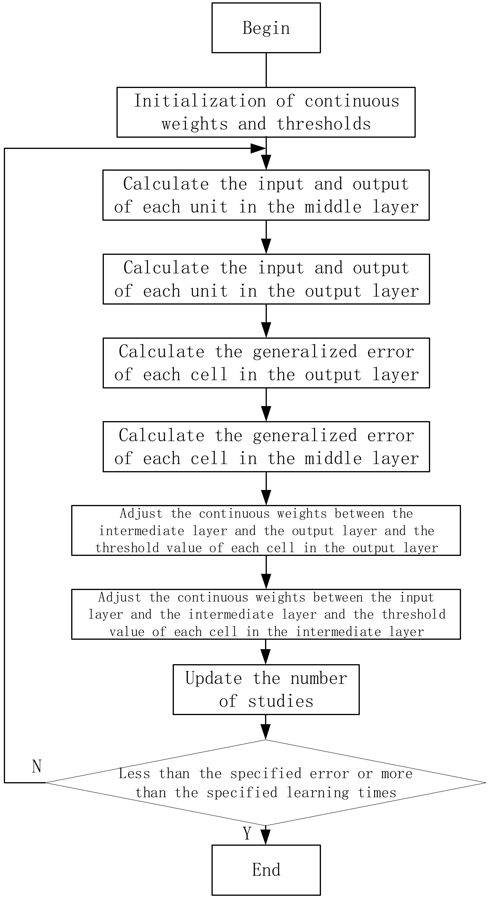
The implementation flow of a BP neural network is shown in Figure 7.

6. Results and Discussion

6.1. SOFC System Experimental Results and Analysis

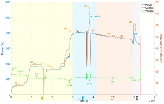
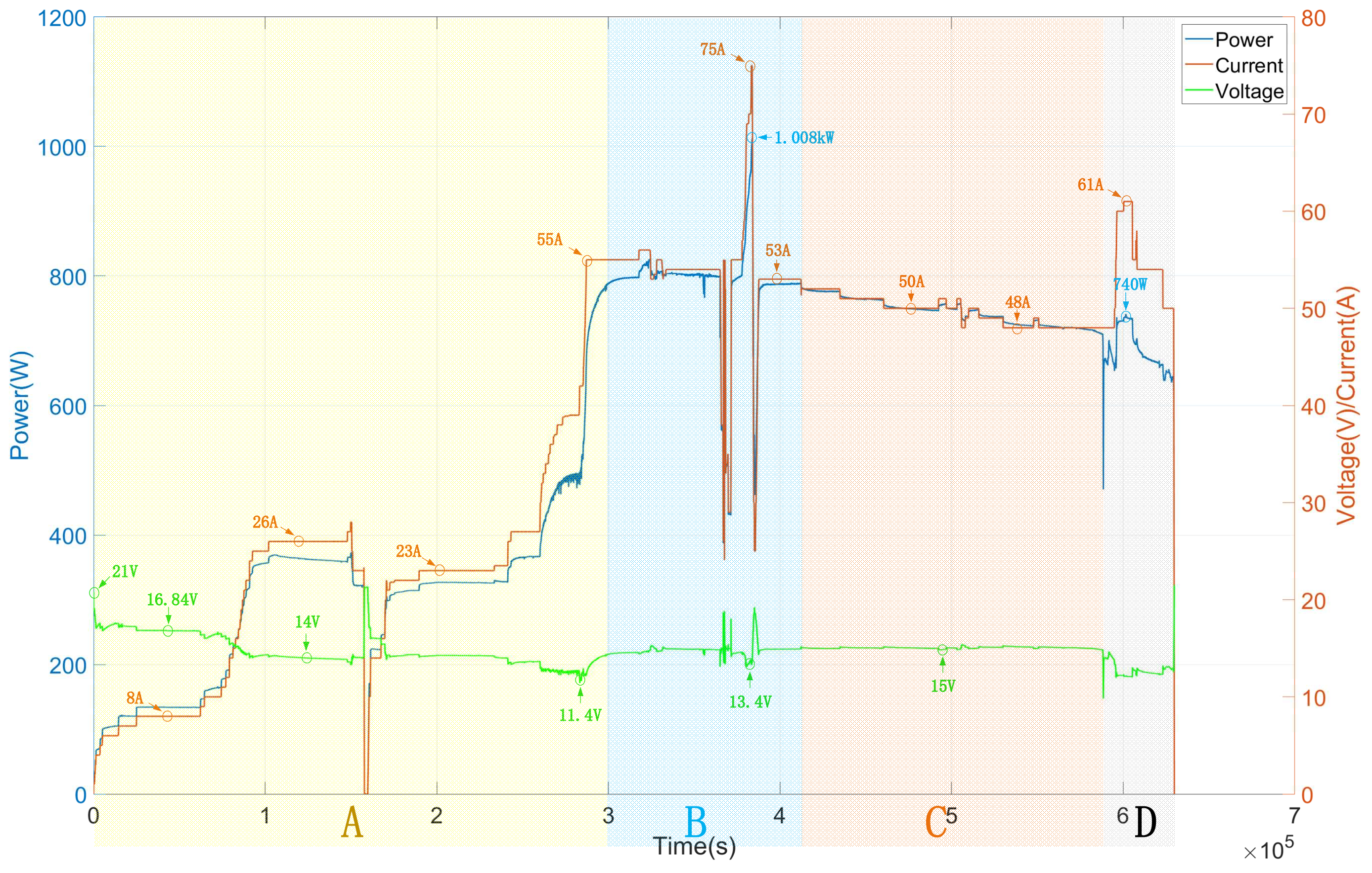
The full-scale experiments of the system include long-term power generation experiments of the stack, gradually from low current to high current. The current, voltage, and power characteristics of the SOFC system for the full working condition experiment are shown in Figure 8.

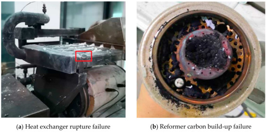
From the experiment, it is known that 0–300,000 s (A) is the current pull-up phase and, after 300,000 s, it is the stable discharge phase. During the stable discharge phase, it is known that the reformer carbon deposition and heat exchanger rupture failure occur in the system based on the change in the system electrical characteristics and the system condition after disassembly, as shown in Figure 9.

Therefore, 300,000–410,000 s (B) is marked as a healthy condition, 410,000–590,000 s (C) is marked as the reformer carbon deposition fault condition, and 590,000 s–shutdown (D) is marked as the heat exchanger rupture fault condition, as shown in

Table 2. SOFC system operation status.

Time	0–300,000 s	300,000–410,000 s	410,000–590,000 s	590,000–Shutdown
Num	A	B	C	D
Status	Current pull-up phase	Health	Reformer carbon deposit failure	Heat exchanger rupture failure

.

The data of each state are divided into two groups, one for fault diagnosis model training and the other for model validation. Among the healthy data, 45,000 data were randomly selected for model training and 5000 data were randomly selected for model validation; among the reformer carbon deposition failure data, 60,000 data were selected for model training and 6000 data were selected for model validation; among the heat exchanger rupture failure, 35,000 data were selected for model training and 5000 data were selected for model validation, as shown in

Table 3. Data for training and validation.

Status	Amount of Training Data	Amount of Test Data
Health	45,000	5000
Reformer carbon deposit failure	60,000	6000
Heat exchanger rupture failure	35,000	5000

.

6.2. Analysis of PCA Data Dimensionality Reduction Results

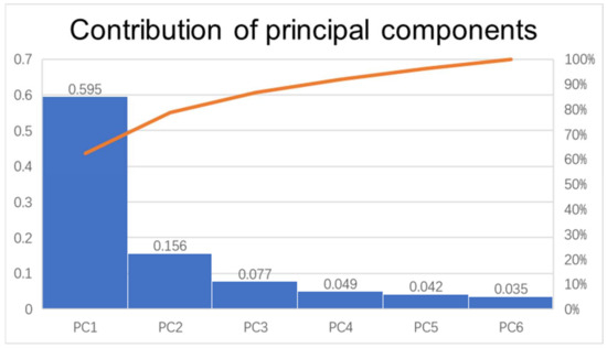
The variables in the SOFC system are coupled with each other, and the variables contain information that is duplicated between them. A small number of principal components extracted from all variables can describe the data characteristics of the whole system, so data dimensionality reduction by PCA can greatly reduce the complexity of the data. After the initial screening, the fuel input flow rate, fuel input flow rate to the combustion chamber, air input flow rate to the reformer, bypass air flow rate, deionized water input flow rate, reformer temperature, heat exchanger temperature, combustion chamber temperature, current, and voltage were selected to indicate the system performance. The reformer temperature was measured by sensors at five different locations and therefore contains five variables; the heat exchanger temperature is represented by six variables; and the combustion chamber temperature is represented by seven variables. Thus, there are a total of 25 variables to describe the performance of the system. PCA dimensionality reduction in these 25 variables revealed that all variables can be represented using six principal components, and Figure 10 represents the contributions of the six principal components.

As can be seen from the above figure, the cumulative contribution of the first six principal components is 95.4%, with principal component 1 accounting for a significantly higher proportion of the contribution than the other principal components, with a value of 59.5%. After feature fusion by PCA, the original 25-dimensional features are reduced to 6-dimensional, and the number of feature dimensions is reduced by 76%, which is a remarkable effect in compressing the amount of information and reducing the number of feature dimensions. PCA-based feature fusion methods are also effective in reducing the training time of classifiers, which is of great value when dealing with massive amounts of data, as shown in the next subsection.

6.3. Comparison of the Results of SVM and BP Neural Network Fault Diagnosis

SVM, BP, LSTM, and RNN classification algorithms are used to compare and analyze the accuracy of fault diagnosis before and after data dimensionality reduction. The classification results are shown in

Table 4. Accuracy of fault diagnosis before and after data downscaling.

	Parameters	Precision	Recall	F1	Time Cost
SVM	Decision function shape = OVR Penalty factor = 1, Kernel = RBF C(1,2,3) = 0.2391, 1.8508, 0.0951 σ(1,2,3) = 4.1167, 9.2878, 687.7935	0.952	0.963	0.957	35.795 s
SVM + PCA		0.998	1	0.998	17.588 s
BP	Input node = 7 Hidden layer node: (16, 64), (64, 256), (256, 256), (256, 32), (32, 7)	0.867	0.864	0.865	145.23 s
BP + PCA		0.909	0.909	0.909	95.47 s
LSTM	Input layer = 7, Hidden layer = 16 Sequence length = 100	0.824	0.826	0.825	378.17
RNN	Input layer = 7, Hidden size = 64 Hidden layer = 8, Sequence length = 100	0.822	0.822	0.822	164.28

.

In order to evaluate the generalization performance of a fault diagnosis model, some metrics to measure the quality of the model are needed. Taking the binary classification problem as an example, the samples are classified into four cases: true positive (TP), false positive (FP), true negative (TN), and false negative (FN), based on the combination of their true categories and the classifier prediction results. TP, FP, TN, and FN denote their corresponding sample numbers, respectively. With these four cases, precision (P), recall (R), and the F1 metric can be calculated.

Precision (P): Precision indicates the proportion of predicted positive samples relative to the true positive samples in the total sample. Its definition is shown as follows:

$$P=\frac{TP}{TP+FP}$$

(9)

Recall (R): Recall indicates how many positive examples in the sample were correctly predicted, and is defined as follows:

$$R=\frac{TP}{TP+FN}$$

(10)

In practical model evaluation, a model cannot be fully evaluated with precision or recall alone; both values of precision/recall must be used to evaluate the model. Therefore, a comprehensive evaluation metric, F1, is introduced, which is defined based on the harmonic mean of precision and recall:

$$F1=\frac{2PR}{P+R}$$

(11)

The research results show that SVM, BP, LSTM, and RNN algorithms are able to obtain a fault recognition rate of more than 80%. The LSTM neural network algorithm has a relatively large time complexity, uses the longest time to complete model training and state identification, and may not be able to complete time-critical online applications. The state recognition accuracy of BP neural network is higher than that of LSTM and RNN models because the feature extraction ability of BP neural network is higher than that of the other two models, and the superior feature extraction ability leads to better classification ability [35]. The SVM model has the highest accuracy in state identification due to its ability to map the problem to a high-dimensional space by means of kernel functions, which yields excellent classification of nonlinear problems. The SVM model has two main hyperparameters that enable constrained optimization to process the outliers and more accurately distinguish between categories.

The dimensionality of the features of the dataset fused by PCA was reduced substantially, and the experimental results of PCA + SVM and PCA + BP showed that the training and classification time of the classifier was greatly reduced and did not affect the accuracy of the classifier. On the contrary, the reduction in redundant features after fusion results in a small increase in accuracy. This is because the system data before dimensionality reduction contain redundant features and features containing error information, which will affect the accuracy of the fault classifier, in addition to increasing the computation of the classifier and increasing the running time of the classifier. The runtime reduction after fusion is very large, which indicates that the simple and effective feature set significantly reduces the computational effort of the classifier.

The combination of PCA and SVM has advantages over other algorithms in terms of diagnostic accuracy and time, with an accuracy of over 99% and a runtime that can be controlled within 20 s. Therefore, the combination of the two can make full use of the complementarity between the features, eliminate the redundant information in the feature information, and maximize the amount of compressed information to improve the ability to characterize the operation status and thus improve the fault diagnosis rate. The method combines the excellent fusion of principal component analysis to remove redundant information and the good classification performance of the support vector machine classifier, which enables the method to achieve feature dimensionality reduction while effectively characterizing the operation status of the equipment. The classifier can be used in future experiments to monitor the operational status of the SOFC system in real time. According to the operation status of the system to provide the corresponding control strategy, when the system again detects the occurrence of a carbon deposition fault, the water-to-carbon ratio of the system should be adjusted in time to prevent further carbon accumulation; when the system again detects the heat exchanger rupture fault, the operation of the system should be stopped immediately and the damaged heat exchanger should be replaced.

7. Conclusions

This paper presents a data-driven fault diagnosis scheme for SOFC systems. This study began with the design of system experiments and performed fault diagnosis on the data obtained from the experiments. First, the system experiments were designed; then, PCA dimensionality reduction was performed using the obtained data; finally, the SVM and BP neural network fault diagnosis models were trained and validated. The experiment yielded a total of 629,999 s of experimental data, with the first 300,000 s being the current pull state, in which a thermal standby occurred at about 150,000 s; the period from 300,000 to 410,000 s was the healthy operation state; a reformer carbon buildup failure occurred in the period from 410,000 to 590,000 s; and a heat exchanger rupture failure occurred at 590,000 s, which led to a system shutdown. These data were divided into training data and test data for fault diagnosis in SVM and BP neural networks. The fault diagnosis results show that both SVM and BP fault diagnosis algorithms can achieve online fault identification. The results of comparing the PCA + SVM algorithm with the SVM, BP, and PCA + BP algorithms show that the PCA + SVM algorithm is superior in terms of running time and accuracy, the diagnostic accuracy can reach more than 99%, and the running time is within 20 s. The program provides a fault diagnosis scheme that provides guidance for subsequent experimental improvements and controller design. Using this solution for subsequent experiments can effectively prevent failures, improve system life, and reduce system costs.

References

- Sharaf, O.Z.; Orhan, M.F. An overview of fuel cell technology: Fundamentals and applications. Renew. Sustain. Energy Rev. 2014, 32, 810–853. [Google Scholar] [CrossRef]
- Kirubakaran, A.; Jain, S.; Nema, R.K. A review on fuel cell technologies and power electronic interface. Renew. Sustain. Energy Rev. 2009, 13, 2430–2440. [Google Scholar] [CrossRef]
- Mekhilef, S.; Saidur, R.; Safari, A. Comparative study of different fuel cell technologies. Renew. Sustain. Energy Rev. 2012, 16, 981–989. [Google Scholar] [CrossRef]
- Harun, N.F.; Shadle, L.; Oryshchyn, D.; Tucker, D. Fuel utilization effects on system efficiency and solid oxide fuel cell performance in gas turbine hybrid systems. Proc. ASME Turbo Expo 2017, 3, 1–12. [Google Scholar] [CrossRef]
- Xia, Z.; Deng, Z.; Jiang, C.; Zhao, D.Q.; Kupecki, J.; Wu, X.L.; Xu, Y.W.; Liu, G.Q.; Fu, X.; Li, X. Modeling and analysis of cross-flow solid oxide electrolysis cell with oxygen electrode/electrolyte interface oxygen pressure characteristics for hydrogen production. J. Power Sources 2022, 529, 231248. [Google Scholar] [CrossRef]
- Boldrin, P.; Brandon, N.P. Progress and outlook for solid oxide fuel cells for transportation applications. Nat. Catal. 2019, 2, 571–577. [Google Scholar] [CrossRef] [Green Version]
- Barelli, L.; Barluzzi, E.; Bidini, G. Diagnosis methodology and technique for solid oxide fuel cells: A review. Int. J. Hydrog. Energy 2013, 38, 5060–5074. [Google Scholar] [CrossRef]
- Lin, R.H.; Xi, X.N.; Wang, P.N.; Wu, B.D.; Tian, S.M. Review on hydrogen fuel cell condition monitoring and prediction methods. Int. J. Hydrog. Energy 2019, 44, 5488–5498. [Google Scholar] [CrossRef]
- Peng, J.; Huang, J.; Wu, X.L.; Xu, Y.W.; Chen, H.; Li, X. Solid oxide fuel cell (SOFC) performance evaluation, fault diagnosis and health control: A review. J. Power Sources 2021, 505, 230058. [Google Scholar] [CrossRef]
- Zheng, Z.; Péra, M.C.; Hissel, D.; Becherif, M.; Agbli, K.S.; Li, Y. A double-fuzzy diagnostic methodology dedicated to online fault diagnosis of proton exchange membrane fuel cell stacks. J. Power Sources 2014, 271, 570–581. [Google Scholar] [CrossRef]
- Gao, Z.; Cecati, C.; Ding, S.X. A survey of fault diagnosis and fault-tolerant techniques-part I: Fault diagnosis with model-based and signal-based approaches. IEEE Trans. Ind. Electron. 2015, 62, 3757–3767. [Google Scholar] [CrossRef] [Green Version]
- Yang, B.; Guo, Z.; Wang, J.; Wang, J.; Zhu, T.; Shu, H.; Qiu, G.; Chen, J.; Zhang, J. Solid oxide fuel cell systems fault diagnosis: Critical summarization, classification, and perspectives. J. Energy Storage 2021, 34, 102153. [Google Scholar] [CrossRef]
- Moser, G.; Costamagna, P.; De Giorgi, A.; Greco, A.; Magistri, L.; Pellaco, L.; Trucco, A. Joint feature and model selection for SVM fault diagnosis in solid oxide fuel cell systems. Math. Probl. Eng. 2015, 2015, 282547. [Google Scholar] [CrossRef]
- Murshed, A.M.; Huang, B.; Nandakumar, K. Monitoring of solid oxide fuel cell systems. Asia-Pac. J. Chem. Eng. 2011, 6, 204–219. [Google Scholar] [CrossRef]
- Polverino, P.; Pianese, C.; Sorrentino, M.; Marra, D. Model-based development of a fault signature matrix to improve solid oxide fuel cell systems on-site diagnosis. J. Power Sources 2015, 280, 320–338. [Google Scholar] [CrossRef]
- Polverino, P.; Sorrentino, M.; Pianese, C. A model-based diagnostic technique to enhance faults isolability in Solid Oxide Fuel Cell systems. Appl. Energy 2017, 204, 1198–1214. [Google Scholar] [CrossRef]
- Polverino, P.; Esposito, A.; Pianese, C.; Ludwig, B.; Iwanschitz, B.; Mai, A. On-line experimental validation of a model-based diagnostic algorithm dedicated to a solid oxide fuel cell system. J. Power Sources 2016, 306, 646–657. [Google Scholar] [CrossRef]
- Gallo, M.; Costabile, C.; Sorrentino, M.; Polverino, P.; Pianese, C. Development and application of a comprehensive model-based methodology for fault mitigation of fuel cell powered systems. Appl. Energy 2020, 279, 115698. [Google Scholar] [CrossRef]
- Wu, X.L.; Xu, Y.W.; Xue, T.; Shuai, J.; Jiang, J.; Deng, Z.; Fu, X.; Li, X. Control-oriented fault detection of solid oxide fuel cell system unknown input on fuel supply. Asian J. Control 2019, 21, 1824–1835. [Google Scholar] [CrossRef]
- Xu, Y.W.; Wu, X.L.; Zhong, X.B.; Zhao, D.Q.; Sorrentino, M.; Jiang, J.; Jiang, C.; Fu, X.; Li, X. Mechanism model-based and data-driven approach for the diagnosis of solid oxide fuel cell stack leakage. Appl. Energy 2021, 286, 116508. [Google Scholar] [CrossRef]
- Fu, X.; Liu, Y.; Li, X. Source diagnosis of solid oxide fuel cell system oscillation based on data drive. Energies 2020, 13, 4069. [Google Scholar] [CrossRef]
- Li, S.; Cao, H.; Yang, Y. Data-driven simultaneous fault diagnosis for solid oxide fuel cell system using multi-label pattern identification. J. Power Sources 2018, 378, 646–659. [Google Scholar] [CrossRef]
- Costamagna, P.; De Giorgi, A.; Moser, G.; Pellaco, L.; Trucco, A. Data-driven fault diagnosis in SOFC-based power plants under off-design operating conditions. Int. J. Hydrog. Energy 2019, 44, 29002–29006. [Google Scholar] [CrossRef]
- Costamagna, P.; De Giorgi, A.; Moser, G.; Serpico, S.B.; Trucco, A. Data-driven techniques for fault diagnosis in power generation plants based on solid oxide fuel cells. Energy Convers. Manag. 2019, 180, 281–291. [Google Scholar] [CrossRef]
- Zheng, Y.; Wu, X.L.; Zhao, D.; Xu, Y.W.; Wang, B.; Zu, Y.; Li, D.; Jiang, J.; Jiang, C.; Fu, X.; et al. Data-driven fault diagnosis method for the safe and stable operation of solid oxide fuel cells system. J. Power Sources 2021, 490, 229561. [Google Scholar] [CrossRef]
- Marra, D.; Sorrentino, M.; Pianese, C.; Iwanschitz, B. A neural network estimator of Solid Oxide Fuel Cell performance for on-field diagnostics and prognostics applications. J. Power Sources 2013, 241, 320–329. [Google Scholar] [CrossRef]
- Wu, X.L.; Xu, Y.W.; Xue, T.; Zhao, D.Q.; Jiang, J.; Deng, Z.; Fu, X.; Li, X. Health state prediction and analysis of SOFC system based on the data-driven entire stage experiment. Appl. Energy 2019, 248, 126–140. [Google Scholar] [CrossRef]
- Zhang, Z.; Li, S.; Xiao, Y.; Yang, Y. Intelligent simultaneous fault diagnosis for solid oxide fuel cell system based on deep learning. Appl. Energy 2019, 233–234, 930–942. [Google Scholar] [CrossRef]
- Wu, X.; Ye, Q. Fault diagnosis and prognostic of solid oxide fuel cells. J. Power Sources 2016, 321, 47–56. [Google Scholar] [CrossRef]
- Zhang, Z.; Li, S.; Yang, Y. A General Approach for Fault Identification in SOFC-based Power Generation Systems. Proc. Am. Control Conf. 2018, 2018, 3816–3821. [Google Scholar] [CrossRef]
- Sinha, V.; Mondal, S. Recent development on performance modelling and fault diagnosis of fuel cell systems. Int. J. Dyn. Control 2018, 6, 511–528. [Google Scholar] [CrossRef]
- Zhang, X.; Zhou, J.; Chen, W. Data-driven fault diagnosis for PEMFC systems of hybrid tram based on deep learning. Int. J. Hydrog. Energy 2020, 45, 13483–13495. [Google Scholar] [CrossRef]
- Xu, P.; Huang, L.; Song, Y. An optimal method based on HOG-SVM for fault detection. Multimed. Tools Appl. 2022, 81, 6995–7010. [Google Scholar] [CrossRef]
- Xiao, M.; Zhang, W.; Zhao, Y.; Xu, X.; Zhou, S. Fault diagnosis of gearbox based on wavelet packet transform and CLSPSO-BP. Multimed. Tools Appl. 2022. [Google Scholar] [CrossRef]
- Li, M.W.; Xu, D.Y.; Geng, J.; Hong, W.C. A ship motion forecasting approach based on empirical mode decomposition method hybrid deep learning network and quantum butterfly optimization algorithm. Nonlinear Dyn. 2022, 107, 2447–2467. [Google Scholar] [CrossRef]
Publisher’s Note: MDPI stays neutral with regard to jurisdictional claims in published maps and institutional affiliations. |
© 2022 by the authors. Licensee MDPI, Basel, Switzerland. This article is an open access article distributed under the terms and conditions of the Creative Commons Attribution (CC BY) license (https://creativecommons.org/licenses/by/4.0/).