Seismic Analysis of 10 MW Offshore Wind Turbine with Large-Diameter Monopile in Consideration of Seabed Liquefaction

Abstract

With the increasing construction of large-scale wind turbines in seismically active coastal areas, the survivability of these high-rated-power offshore wind turbines (OWTs) in marine and geological conditions becomes extremely important. Although research on the dynamic behaviors of OWTs under earthquakes has been conducted with consideration of the soil-structure interaction, the attention paid to the impact of earthquake-induced seabed liquefaction on OWTs supported by large-diameter monopiles remains limited. In view of this research gap, this study carries out dynamic analyses of a 10 MW OWT under combined wind, wave, and earthquake loadings. This study uses a pressure-dependent multisurface elastoplastic constitutive model to simulate the soil liquefaction phenomenon. The results indicate that the motion of the large-diameter monopile leads to more extensive soil liquefaction surrounding the monopile, specifically in the zone near the pile toe. Moreover, compared with earthquake loading alone, liquefaction becomes more severe under the coupled wind and earthquake loadings. Accordingly, the dynamic responses of the OWT are apparently amplified, which demonstrates the importance of considering the coupling loadings. Compared with wind loading, the effect of wave loading on the dynamic response and liquefaction potential is relatively insignificant.

1. Introduction

The contradiction between the plan to increase energy consumption and reduce the carbon footprint has motivated many countries to explore more sustainable and renewable energy sources, including wind, solar, hydropower, geothermal, and biomass. In the past several decades and since the oil crisis in the early 1970s, wind energy has rapidly developed worldwide. Moreover, many onshore and offshore wind farms have been constructed or are being planned, specifically in Europe, the United States, and Asia. Figure 1 presents the development history of the total installation of wind turbines (WTs) in the world. The accumulated wind power capacity reached approximately 743 GW in 2020, with 35.0 GW for offshore WTs, which accounted for 4.5% of the total capacity [1].

Several distinct trends are witnessed in the current WT market. The first is the increasing installation of WTs in coastal areas [2,3]. Offshore wind turbines (OWTs) have become mainstream because of their inherent advantages, such as higher and steadier wind speeds, adequate installation space, and less visual and noise impacts. The second trend is the extensive construction of wind farms in seismic-prone areas because of the larger population sizes and energy requirements in these specific zones, such as China, Japan, and India [4,5]. The third trend is the improvement of energy capture by using increasingly larger turbine structures [6]. For example, the most powerful WT prototype (the GE 12-MW Halidae-X) has recently produced the first power at the Rotterdam-Maasvlakte port in the Netherlands [7]. The last trend is the use of various foundation types for bottom-fixed and floating OWTs, of which monopiles are still the most common choice because of their simpler shape, easier installation, and better economic benefits [8,9,10,11,12].

Given these development trends, high-power OWTs that are supported by large-diameter monopiles in active seismic zones present new design requirements and challenges. For example, on the basis of wind field data over 38 years (from 1979 to 2016), Wan et al. [13] investigated the wind energy potential of the South China Sea (Figure 2a). They concluded that the climatic and geographic circumstances in the Taiwan Strait are highly favorable for wind power development. The average wind power density of the Taiwan Strait reaches approximately 450 W/m² because of the monsoon influence and the strait narrowing effect. Numerous wind plants have been planned or constructed, such as the Xinghua Bay Wind Farm and the Chang-Bin Wind Farm. Meanwhile, the strait is located between the Eurasian Plate and the Philippine Sea Plate, and it represents the region with the highest seismicity [14], as depicted in Figure 2b. Therefore, the new installations will be susceptible to coupled wind, wave, and earthquake loadings.

The existing research on WTs that are subjected to seismic loadings mainly covers three aspects. The first is the dynamic responses of onshore WTs under wind and earthquake loadings, or offshore WTs under wind, wave, and earthquake loadings with consideration of the aerodynamic damping, and the seismic loading conditions and types [15,16,17,18,19,20,21,22,23]. The second aspect is the fragility analysis and the collapse evaluation, which employs the nonlinear incremental dynamic analysis approach to assess the exceeding probability for various damage states [24,25,26,27,28]. Finally, the third aspect is the frequency variation and dynamic performance with consideration of the soil–structure interaction (SSI) by employing three conventional simplified models: apparent fixity, coupled springs, and distributed springs [29,30,31,32,33,34].

The general conclusion, that seismic loading on WTs is insignificant compared with wind loadings, has been drawn in the literature [35]. However, this conclusion needs to be carefully revisited, particularly for OWTs, given that the liquefaction risk has often been overlooked in the aforementioned literature. The geotechnical investigation of the Chang-Bin Wind Farm [36,37] points out that the seabed was mainly composed of silty sand and low plasticity clay, with loose-to-medium sand that existed in the upper 25 m layer. Standard penetration tests clarified that the liquefaction thickness was more than 15 m. Earthquake-induced liquefaction was observed during numerous strong earthquakes, such as the 1964 Niigata (Japan), 1964 Alaska (USA), 1999 Chichi (Taiwan), 1999 Kocaeli (Turkey), 2008 Wenchuan (China), and 2011 Christchurch (New Zealand) earthquakes [38]. Field investigations, laboratory tests, and numerical simulations have been conducted to evaluate the liquefaction potential and the possible consequences. These studies include initial liquefaction, pore water pressure generation, soil lateral spreading and settlement, and pile bending moment variation [39]. When coupled with considerable wind and wave loadings, ground liquefaction may pose a potential risk to irreversible permanent deflection, or even to structural stability, which certainly warrants research attention.

Despite the significant effects on a single pile–soil system, liquefaction evaluation studies for OWTs remain limited. Barari et al. [40] employed the University of California San Diego (UCSD) sand model to investigate small monopile-supported OWTs under cyclic loads with different cycle numbers and frequencies. Using the same soil model, Patra and Haldar [41] examined the influence of various loadings on liquefaction by considering an artificial seismic record, and further evaluated the dynamic responses considering different parameters, which included the peak acceleration values, the embedded depths of the monopile, and the sand deposit depths [42,43]. Kementzetzidis et al. [44] adopted the SANISAND04 model to investigate the geotechnical dynamics of an 8 MW OWT with a monopile foundation under coupled wind and wave loadings. For other types of foundations, Zhang et al. [45,46] analyzed the seismic responses and antiliquefaction performances of WTs with a prestressed concrete bucket foundation by using the Seed simplified method [47,48] and different finite element (FE) software (e.g., ADINA and ABAQUS). Gao et al. [49] also adopted the suction bucket foundation to study the failure mechanism of WTs by employing the finite element–finite difference (FE-FD) method with a cyclic mobility constitutive model, and they indicated that the permanent displacement could reach around 40% of the safety threshold. Esfeh and Kaynia [50] conducted a liquefaction assessment for a floating WT, which was fixed on the seabed with the anchor pile and anchor suction, by using the finite-difference code, FLAC3D, and Kobe-L seismic records. A similar caisson foundation concept was developed and employed to evaluate the liquefaction distribution and dynamic performance of a fixed-bottom wind turbine [51,52]. Tsiapas et al. [53] and Chaloulos et al. [54] depict the degradation of the pseudostatic safety factor against the pullout failure of pile-supported tension leg platforms with consideration to the seabed liquefaction. Moreover, the dynamic performance of OWTs with a monopile foundation under the wave-induced liquefaction condition was analyzed by Fard et al. [55], with different structure and load parameters, including the pile diameters, the embedment depths, and the sea-wave periods and depths. Li et al. [56] and Wang et al. [57,58] carried out a series of geotechnical centrifuge tests of the newly developed suction bucket and hybrid monopile foundations in dry and saturated soil conditions. Then, they evaluated the liquefaction resistance effectiveness of these foundations on the basis of the soil seismic behavior and the superstructure dynamic response. A shake table test of a 1/25 scale model of the 5 MW offshore wind turbine supported by a piled jacket foundation was conducted by Ko et al. [59] and Ko and Li [60] to describe the interaction mechanism between the soil and the piles during liquefaction.

However, some questions remain unanswered in the literature. First, numerous simulations and experiments were focused on small-diameter monopiles. However, the soil–pile interaction and liquefaction mechanism for high-rated-power OWTs that are supported by large-diameter monopiles have not been systematically investigated. Second, with the increasing rotor diameter and hub height, the wind loading plays a more critical role in the ultimate-limit-state and serviceability-limit-state design. The coupling of wind, wave, and earthquake loadings under different operating conditions may influence the liquefaction depth, which has not been discussed so far. This study aims to answer these fundamental questions by employing the Technical University of Denmark (DTU) 10 MW benchmark WT model, which is supported on a monopile with a large diameter of 10 m. The detailed FE model was established in the software, OpenSees, by using an advanced soil constitutive model to capture the variation in the excess pore water pressure (EPP) and the liquefaction depth. Three loading scenarios, including five earthquake records, instantaneous wind loading with earthquake records, and wind–wave–earthquake coupling loading, were simulated.

This study is organized into five sections. Following the introduction in Section 1, Section 2 presents the numerical modeling of the DTU 10 MW WT. This section also introduces a multisurface constitutive model that describes the effective soil stress and the damping model with consideration of the structural and loading characteristics. Section 3 concisely describes the earthquake, wind, and wave loadings, as well as the corresponding modeling procedure. Section 4 focuses on the liquefaction development and the dynamic response by comparing the soil and pile performances in different loading scenarios. Section 5 concludes the study and summarizes the findings.

2. Numerical Modeling of OWT

2.1. DTU 10 MW Reference WT

Two reference WT models, namely, a National Renewable Energy Laboratory (NREL) 5 MW WT, and a DTU 10 MW WT, are commonly employed to assess the dynamic performance of OWTs under complex environmental loadings. To reduce the levelized cost of energy, the rated power is continuously enhanced by increasing the blade length and the tower height. Given this development trend, the DTU 10 MW OWT, with a large-diameter monopile foundation, which was proposed by Bak et al. [61] and Velarde [62], is selected as an example in this study. The outer diameter of the tower varies linearly from 8.3 m at the bottom, to 5.5 m at the top. The tower is divided into ten sections, where the wall thickness of each section is assumed to be constant. Velarde [62] suggests that the tower diameter of each section should be increased with the same factor of 1.25 in order to satisfy the fundamental frequency requirement of the entire system, whereas the wall thicknesses are kept unchanged. The total length of the monopile is 75 m, of which 40 m is in seawater, and 35 m is embedded in the seabed. The monopile diameter is 10 m, and the wall thickness is assumed to be 1/80 of the monopile diameter, which is approximately 0.125 m.

2.2. Structural Modeling

The complete three-dimensional FE model is built using an open-source FE code, OpenSees (Version 2.5.0), for the seismic simulations, as is shown in Figure 3. The rotor–nacelle assembly (RNA) that is fixed at the top of the tower is represented by lumped mass points in order to simplify the computation. The transition piece (TP) is also modeled as a lumped mass that is attached to the tower node, with a height of 19.0 m above sea level.

Table 1. Main parameters of the FE model [61,62].

DTU 10 MW Reference WT with Large-Diameter Monopile
Basic description	Rated power	10 MW
	Cut-in, rated, cut-out wind speeds	4 m/s, 11.4 m/s, 25 m/s
	Minimum, maximum rotor speeds	6.0 rpm, 9.6 rpm
Rotor–nacelle assembly	Single blade mass	40,699 kg
	Hub mass	105,520 kg
	Nacelle mass	446,036 kg
	Blade structural damping ratio	0.48%
Tower	Height above water	115.63 m
	Tower diameter	10.375 m (bottom), 6.875 m (top)
	Wall thickness (10 sections from bottom to top)	0.038 m, 0.036 m, 0.032 m, 0.034 m, 0.030 m, 0.028 m, 0.026 m, 0.024 m, 0.022 m, 0.020 m
	Integrated mass	786,223 kg
	Structural damping ratio	1%
Transition piece	Integrated mass	500,000 kg
Monopile	Length	40 m (in water); 35 m (in soil)
	Diameter	10 m
	Wall thickness	0.125 m
	Integrated mass	2,554,000 kg
	Structural damping ratio	1%
Soil domain	Length	100 m
	Width	100 m
	Depth	55 m

shows that the masses of the rotor, the nacelle, and the TP are 227,962, 446,036, and 500,000 kg, respectively. The tower density is assumed to be 8500 kg/m³, with consideration of the paint, welds, bolts, and flanges, whereas the monopile density that is embedded in the soil is considered to be 7885 kg/m³. The tower and monopile are modeled by the elastic beam–column element with 12 degrees of freedom (DOFs), and they are divided into 129 and 47 elements, respectively, with an element size of approximately 1.0 m.

The vibration of the monopile in seawater accelerates the surrounding water, and the water–monopile interaction can be modeled by using the added mass approach, as suggested by [63] and [64]. The tributary mass is only valid in the horizontal translational direction. The effective mass ($m_e$) on the monopile nodes in the water can be expressed as:

$$m_e=m_{monopile}+m_{add},$$

(1)

$$m_{add}=C_a{A}_p{\rho }_w,$$

(2)

where $m_{monopile}$ is the physical mass of the monopile; $m_{add}$ is the added mass; $C_a$ is the added mass coefficient, which is assumed to be 1.0, as suggested in [65]; $A_p$ is the cross section of the monopile; and ${\rho }_w=1030{ \mathrm{kg}/\mathrm{m}}^3$ is the seawater density.

2.3. Soil Modeling

The adoption of nonlinear springs (as is recommended in [66,67]) to model the soil domain prevents the proper evaluation of the liquefaction risk. The nonlinear p–y method is a widely adopted model in the studies of the SSI of OWTs. Although this method could be extended to the dynamic analysis of foundations in liquefiable soil by considering the dynamically evolved soil properties, this approach cannot capture the pore water pressure. Therefore, three-dimensional FE-FD approaches are widely employed for liquefaction evaluation with appropriate soil constitutive models. Lu et al. [68] and Qiu et al. [69] summarize several advanced soil constitutive models, including pressure-independent models (e.g., PressureIndependMultiYield and PressureIndependMultiYieldSoftening) and pressure-dependent models (e.g., PressureDependMultiYield, PressureDependMultiYield02, PressureDependMultiYield03, and LadeDuncanMultiYield). These models were developed in the UCSD on the basis of the multisurface models that were suggested by Prevost [70,71]. They presented the model applications in some typical pile-supported multispan bridges and wharves. Then, Zhang et al. [72] employed this elastic–perfectly plastic model to study the effects of the peak ground velocity on the pile–soil system’s response on a liquefiable site. Cheng and Jeremić [73] adopted the boundary surface model that was presented by Dafalias and Manzari [74] and Manzari and Dafalias [75], and the u-p-U constitutive formulation to validate its effectiveness for liquefaction analysis. Rahmani and Pak [76] further demonstrated the efficiency of this model by comparing the numerical results and experimental outcomes of Wilson [77]. On the basis of the concept of the reversible and irreversible components of the volumetric strain, Wang et al. [78,79] constructed two Tsinghua sand models, which were employed to simulate the pre- and post-liquefaction phenomenon for the single and group pile foundation in the liquefied soil. Considering the inconsistent stress distribution and the scaling similarity problems in the shake table and centrifuge tests, numerical simulation is still regarded as the predominant choice for a liquefaction assessment on a full-scale prototype.

The UCSD constitutive model (i.e., the PressureDependentMultiYield material in OpenSees) is employed in this study to describe the soil liquefaction [80,81]. Figure 4 shows the schematic of the constitutive model. In this constitutive model, the plasticity is formulated on the basis of the multisurface concept (Drucker–Prager type), with a nonassociative flow rule to reproduce the dilatancy effect. The model parameters for saturated medium sand that were suggested by Yang et al. [81] are employed in this study, considering the aforementioned geotechnical reports of the Chang-Bin Wind Farm.

Table 2. Model parameters of medium sand [81].

Parameters	Values
Relative density	35–65%
Saturated soil mass density (kg/m3)	1900
Reference low-strain shear modulus (kPa)	75,000
Reference bulk modulus (kPa)	200,000
Friction angle (in degrees)	33
Peak shear strain at peak shear strength (−)	0.1
Reference mean effective confining pressure (kPa)	80
Constant defining various shear and bulk modulus	0.5
Phase transformation angle (in degrees)	27
Constant defining the rate of shear-induced volume contraction or pore pressure built up	0.07
Constant 1 defining the rate of shear-induced volume dilation	0.4
Constant 2 defining the rate of shear-induced volume dilation	2
Parameter 1 controlling the mechanism of liquefaction-induced perfectly plastic shear strain accumulation (kPa)	10
Parameter 2 controlling the mechanism of liquefaction-induced perfectly plastic shear strain accumulation	0.01
Parameter 3 controlling the mechanism of liquefaction-induced perfectly plastic shear strain accumulation	1
Number of yield surfaces	20
Initial void ratio	0.6
Numerical constant	0.7

presents the corresponding model parameters of the adopted medium sand.

As shown in Figure 3 and Table 1, the length and width of the soil domain are assumed to be 100 m, which is ten times the monopile diameter, whereas the depth is 55 m, which is approximately 1.5 times the pile length. This depth was adopted per the suggestion of Barari et al. [40] in order to achieve a good balance between the computing efficiency and the accuracy. The soil domain is modeled by eight-node BrickUP elements with four DOFs for each node, wherein DOFs 1–3 are for the node displacements, and DOF 4 is for the fluid pressure. The mesh size in the vertical direction is set to 5.0 m, whereas different mesh sizes (2.5, 5.0, and 10.0 m) are adopted in the horizontal direction, as suggested by Chiaramonte et al. [82]. Figure 3 shows the detailed mesh information, where fine and coarse meshes are used in the domains close to and far from the monopiles, respectively. A simplified approach, the rigid beam–column links (radially rigid “spikes”) that connect the pile and soil nodes, is employed to model the interaction between the monopile and the surrounding soil. This method was initially adopted by Law and Lam [83] to a large pile group, and was then extended by Elgamal et al. [84] to simulate and evaluate the seismic response and liquefaction potential of the Humboldt Bay Bridge. The monopile and rigid link nodes are connected directly to the surrounding soil nodes by using the EqualDOF command for translational DOFs only.

This paper mainly focuses on the scenario where various dynamic loads are applied in the same direction, which is regarded as the most critical scenario, as is briefly explained in Section 4.1. Considering the symmetry of the model and the loads, only half of the system is modeled in this scenario to improve the computational efficiency. All of the DOFs of the meshes at the bottom boundary are restrained, which represent the bedrock layer. The displacements within the symmetry plane are free, whereas the component that is normal to the symmetry plane is restrained. The horizontal DOFs of the soil nodes on the two-side boundaries are tied together on the same level. In particular, the static water pressure caused by 40 m seawater is also considered and added to DOF 4 of the soil nodes on the seabed surface. Transformation is adopted for the Constraint Handle in OpenSees, and SparseSYM and ProfileSPD are selected for the System of Equations in the nonlinear dynamic and eigenvalue analyses, respectively.

2.4. Modal Properties

Eigenvalue analyses were conducted to examine the dynamic properties (i.e., the modal frequencies and mode shapes) of the OWT system. The obtained modes, 1, 2, and 6, with the frequencies of 0.287, 1.256, and 3.091 Hz correspond to the first-, second-, and third-tower fore–aft frequencies, respectively. The first frequency is slightly higher than the value of 0.25 Hz that is reported by Velarde [62]. The discrepancy may be attributed to the different SSI simulation approaches. The simulated fundamental frequency in this study still lies in between the rotational frequency range, 1P (0.104–0.167 Hz), and the blade passing frequency range, 3P (0.312–0.501 Hz).

2.5. System Damping

The damping mechanism of an OWT is quite complicated. The damping usually comprises structural, aerodynamic, hydrodynamic, and soil damping, which accounts for the contributions of the superstructure, the wind, the waves, the current, and the soil, respectively. Aerodynamic damping results from the interaction between the wind and the rotating blades, and it varies with the operational conditions. In the parked state, the blades are pitched to the maximum pitch angle, and the aerodynamic damping is minimal and negligible. By contrast, the aerodynamic damping is high in normal operating conditions. The aerodynamic damping ratio in the fore–aft direction for an in-operation WT is generally in the range of 1–6% [85]. Hydrodynamic damping develops from the drag between the monopile and the surrounding water, which includes radiation and viscous damping. The upper values of the radiation and viscous damping ratios that are specified in Germanischer Lloyd are 0.22 and 0.15%, respectively [86]. The soil damping is from the SSI, which consists of material and wave radiation damping. In the research of [87], wave radiation damping was neglected, and a constant of 1% of the soil damping ratio was adopted. Structural damping includes material damping and the damping from vibration control systems. The material damping ratio of the steel tower and the monopile is suggested to be 0.3% [61]. The vibration control system is not introduced herein, and the corresponding ratio is not considered. If we sum all the above components, then the damping ratios of the OWT in the parked and operating conditions are equal to 1.7 and 5.2%, respectively. However, in the nonlinear response history analysis (RHA), such a direct superposition of the damping ratios would overestimate the total damping of the OWT system. As suggested by Ali et al. [88] and De Risi et al. [63], constant damping ratios of 1.5 and 3.0% are chosen for the parked and operating OWT, respectively, in this study.

Rayleigh damping is the most common model in the RHA, and the following equations could be adopted to estimate the mass and stiffness coefficients:

$$\alpha =2\zeta \frac{{\omega }_a{\omega }_b}{{\omega }_a+{\omega }_b},\hspace{1em} \beta =2\zeta \frac{1}{{\omega }_a+{\omega }_b},$$

(3)

where $\alpha$ and $\beta$ are the mass and stiffness coefficients, respectively, and ${\omega }_a$ and ${\omega }_b$ are the two selected frequencies with the target damping ratio, $\zeta$. The fundamental frequency (${\omega }_1$) of the structures, and the predominant frequency (${\omega }_{ep}$) of the ground motions, as shown in

Table 3. Selected earthquake records.

No.	Year	Magnitude	Earthquake Event	Station Name	Peak Ground Acceleration (PGA) (g)	Predominant Frequency (Hz)
E1	1979	6.53	Imperial Valley	El Centro Array No.11	0.38	3.78
E2	1994	6.69	Northbridge	Canyon Country-W Lost Canyon	0.48	1.42
E3	1995	6.90	Kobe	Shin-Osaka	0.23	0.81
E4	1999	6.20	Chi-Chi	CHY101	0.18	0.59
E5	2004	6.00	Parkfield	Parkfield-Froelich	0.46	7.40

, are suggested by QUAD4M to be used to consider the excitation characteristics, where QUAD4M is a computer program to evaluate the seismic responses of soil structures [89].

3. Dynamic Loading Cases

In IEC 61400-3-1 [90], five different types of loads should be included for the design calculation: (1) Gravitational and inertial loads, which include static and dynamic loads that result from gravity, vibration, rotation, and earthquake; (2) Aerodynamic loads, which involve static and dynamic loads that are caused by the airflow and its interaction with the stationary and moving parts of WTs; (3) The actuation load, which results from the control system of WTs; (4) Hydrodynamic loads, which are caused by the water flow and its interaction with the support structure; and (5) Ice loads, which act on the foundation. As this study focuses on the influence of earthquakes on the liquefaction risk, the dynamic complexity that arises from the ice loads and the control system (e.g., the pitch and yaw system) is not included.

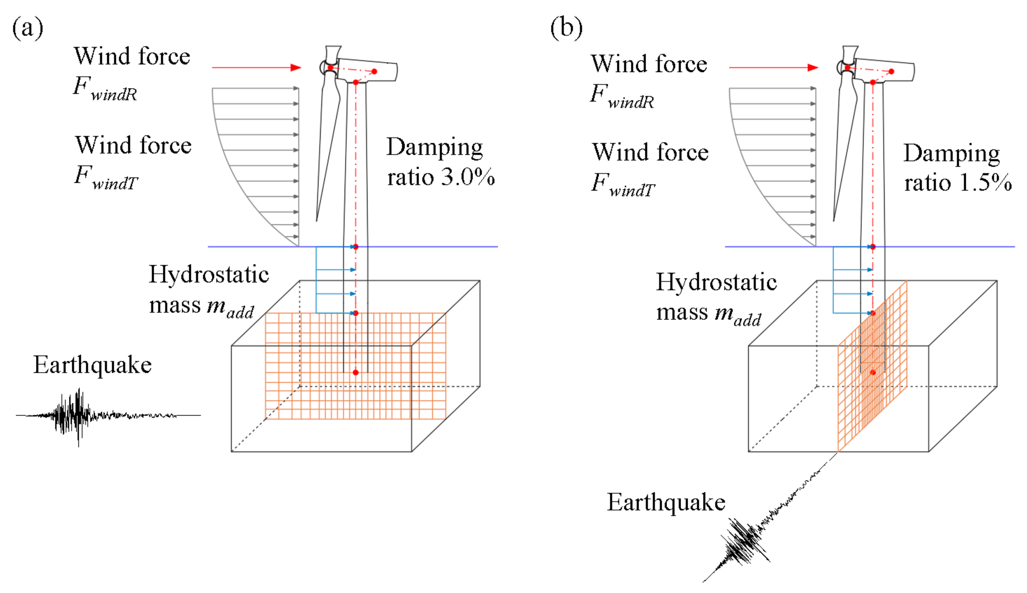
3.1. Inertial Loading

As listed in Table 1, the structural weight is composed of the masses of different components, which include the masses of the RNA, the tower, the monopile, and the transition section. In this study, the tower and the monopile are assumed to interface at the mean sea level. The water surrounding the monopile is modeled by the added mass method with a coefficient of 1.0, as is described in Section 2.2. The soil domain is simulated by the continuum elements, in which the gravitational forces are added automatically in OpenSees.

3.2. Wind Loading

The wind load along the tower is applied to the tower nodes in the x-direction. The thrust force that is imposed on the hub is extracted from the fatigue, aerodynamic, structures, and turbulence (FAST) code [91], which was developed by NREL in the United States. A regular wind profile at a rated wind speed is considered, which is more likely to occur during the entire lifetime of WTs, and is more realistic than storms and hurricanes when an earthquake occurs.

The wind action along the tower is proportional to the wind velocity profile, as is described by the following formula in IEC 61400-3-1 [90]:

$$v(z)=v_{hub}{(\frac{z}{h_{hub}})}^{0.14},$$

(4)

where $h_{hub}$ is the height of the hub center measured from the sea surface; $v_{hub}$ is the velocity at the hub height and is assumed to be the rated wind speed (i.e., 11.4 m/s); and $z$ and $v(z)$ are the height and the wind velocity of the concerned tower node, respectively. Then, the velocity could be employed to calculate the horizontal forces through the following equation:

$$F_{windT}(z)=0.5{\rho }_a{v}^2(z)A(z),$$

(5)

where ${\rho }_a$ is the air density, which is typically equal to 1.225 kg/m³; and $A(z)$ is the tributary area.

Two methods are usually adopted to evaluate the resultant aerodynamic force. One is a simplified method that considers the thrust coefficient. In this approach, Equations (6) and (7) could be employed to estimate this static force on the basis of Frohboese et al. [92] and Arany et al. [93]:

$$F_{windR}=0.5C_T{\rho }_a{v}_{hub}^2{A}_{swept},$$

(6)

$$C_T=\frac{3.5(2V_{hub}+3.5)}{V_{hub}^2},$$

(7)

where $C_T$ is the thrust coefficient; ${\rho }_a$ is the air density; $v_{hub}$ is the velocity at the hub height; $A_{swept}$ is the rotor-swept area; and $V_{hub}$ is the rated wind speed.

The other method is the blade element momentum (BEM) theory, which considers the appropriate wind speed information. This method, which is incorporated in the FAST, is adopted in the following simulation, wherein the Kaimal spectrum is employed to produce the wind field, and the BEM theory is utilized to calculate the aerodynamic loading along the blade. The Kaimal spectrum for three wind components (K = u, v, and w) [94] is shown below:

$$S_K(f)=\frac{4{\sigma }_K^2{L}_K/{\overline{u}}_{hub}}{{(1+6f{L}_K/{\overline{u}}_{hub})}^{5/3}},$$

(8)

$$L_K=\left\{\begin{array}{ll}8.10{\Lambda }_U& K=u\\ 2.70{\Lambda }_U& K=v\\ 0.66{\Lambda }_U& K=w\end{array}\right.,$$

(9)

$${\Lambda }_U=\left\{\begin{array}{ll}0.7z_{hub}& z\le 60 \mathrm{m}\\ 42 \mathrm{m}& z\ge 60 \mathrm{m}\end{array}\right.,$$

(10)

$${\sigma }_v=0.8{\sigma }_u, {\sigma }_w=0.5{\sigma }_u,$$

(11)

where $f$ is the wind frequency; $L_K$ is an integral scale parameter; ${\overline{u}}_{hub}$ is the mean wind speed corresponding to the hub height ($z_{hub}$); ${\Lambda }_U$ is the turbulence scale parameter; and ${\sigma }_K$ is the ambient turbulence standard deviation in three directions. In addition, the spatial coherence model is adopted to add the correlations between the same wind components at two spatially separated points. The IEC equations for the three components [94] shown below are considered:

$$Co{h}_{i,j}{}_K=\exp \left(-a_K\sqrt{{\left(\frac{fd}{{\overline{u}}_{hub}}\right)}^2+{(b_{K}d)}^2}\right),$$

(12)

$$\left\{\begin{array}{l}{a}_u=12,b_u=\frac{0.12}{5.67*60}\\ a_v=\mathrm{large} \mathrm{number}, b_v=0\\ a_w=\mathrm{large} \mathrm{number}, b_w=0\end{array}\right.,$$

(13)

where $f$ is the wind frequency; $d$ is the distance between two concerned spatial points (i and j); and $a_K$ and $b_K$ are the input coherence decrement and the offset parameters, respectively. Following the constructed wind field, the local lift and drag force on each blade element could be computed using the BEM theory [95]:

$$d{F}_L(r,t)=\frac{1}{2}{\rho }_a{V}_{rel}^{2}c(r)C_l(\alpha )dr,$$

(14)

$$d{F}_D(r,t)=\frac{1}{2}{\rho }_a{V}_{rel}^{2}c(r)C_d(\alpha )dr,$$

(15)

$$V_{rel}(r,t)=\sqrt{{\left(\left(V_0(r,t)(1-a)\right)+\tilde{w}(t)\right)}^2+{\left(\Omega \mathrm{r}\left(1+a^{\prime }\right)\right)}^2},$$

(16)

where $r$ is the radial distance of the considered element from the center of the hub; $C_l(\alpha )$ and $C_d(\alpha )$ are the lift and drag coefficients, respectively, which are determined on the basis of the angle of attack ($\alpha$); and $c(r)$ is the chord length. $V_{rel}(r,t)$ is the relative wind velocity, which is defined according to the instantaneous wind speed ($V_0(r,t)$), the stochastic component of wind flow ($\tilde{w}(t)$) and the rotation velocity ($\Omega$). $a$ and $a^{\prime }$ are the axial and tangential induction factors. Finally, the total blade force could be determined by the computational integration along the blade and, consequently, the resultant aerodynamic force could also be defined. Figure 5a shows the calculated resultant force–time history that was extracted from the FAST, and the equivalent static force that is based on Frohboese’s method at the hub. Given that the short duration of the selected seismic records is only 30 s, only a short window (around 37 s) of the wind loading was chosen for the dynamic analyses under the coupled loadings.

3.3. Wave Loading

The wave load imposed on the monopile is also considered in this study. The power spectral density (PSD) of the sea elevation can be described by the JONSWAP spectrum [96]:

$$S(w)=a^{*}{H}_s^2\frac{w^{-5}}{w_p^{-4}}\exp \left(-\frac{5}{4}{(\frac{w}{w_p})}^{-4}\right){\gamma }^{\exp \left(\frac{{\left(w-w_p\right)}^2}{2{\tau }^2{w}_p^2}\right)},$$

(17)

where $w$ is the circular frequency in rad/s; $H_s$ is the significant wave height; $w_p$ is the peak wave frequency; and Parameter $a^{*}$ is calculated by:

$$a^{*}=\frac{0.0624}{0.230+0.0336\gamma -0.185{\left(1.9+\gamma \right)}^{-1}},$$

(18)

where $\gamma$ is the peak enhancement factor (generally taken as 3.3); and $\tau$ is a shape parameter. When $w\le w_p$, $\tau =0.07$; while $\tau =0.09$ for $w>w_p$. In the wave load simulation, the peak wave frequency and the significant wave height are adopted as 0.96 rad/s and 1.9 m, respectively.

After the PSD of the sea surface elevation is determined, the sea surface elevation time history can be simulated by using the inverse fast Fourier transform (IFFT) technique. Thereby, the hydrodynamic load on each monopile element can be calculated by using the Morison formula [96]:

$$\mathrm{d}{F}_{wave}=\frac{1}{2}{\rho }_w{C}_{D}D\left|\dot{x}\right|\dot{x}dz+{\rho }_w{C}_M\pi \frac{D^2}{4}\ddot{x}dz,$$

(19)

where ${\rho }_w$ is the seawater density; $C_D$ and $C_M$ are the drag and inertia coefficients, respectively, which are taken as 1.2 and 2.0, respectively, in this study; $\dot{x}$ and $\ddot{x}$ are the horizontal water particle velocity and the acceleration, respectively; and $D$ is the outer diameter of the monopile. The monopile in the water is equally divided into 40 segments with a length of 1.0 m, to simplify the calculation. The representative wave loads at the mean sea level and the mudline are shown in Figure 5b.

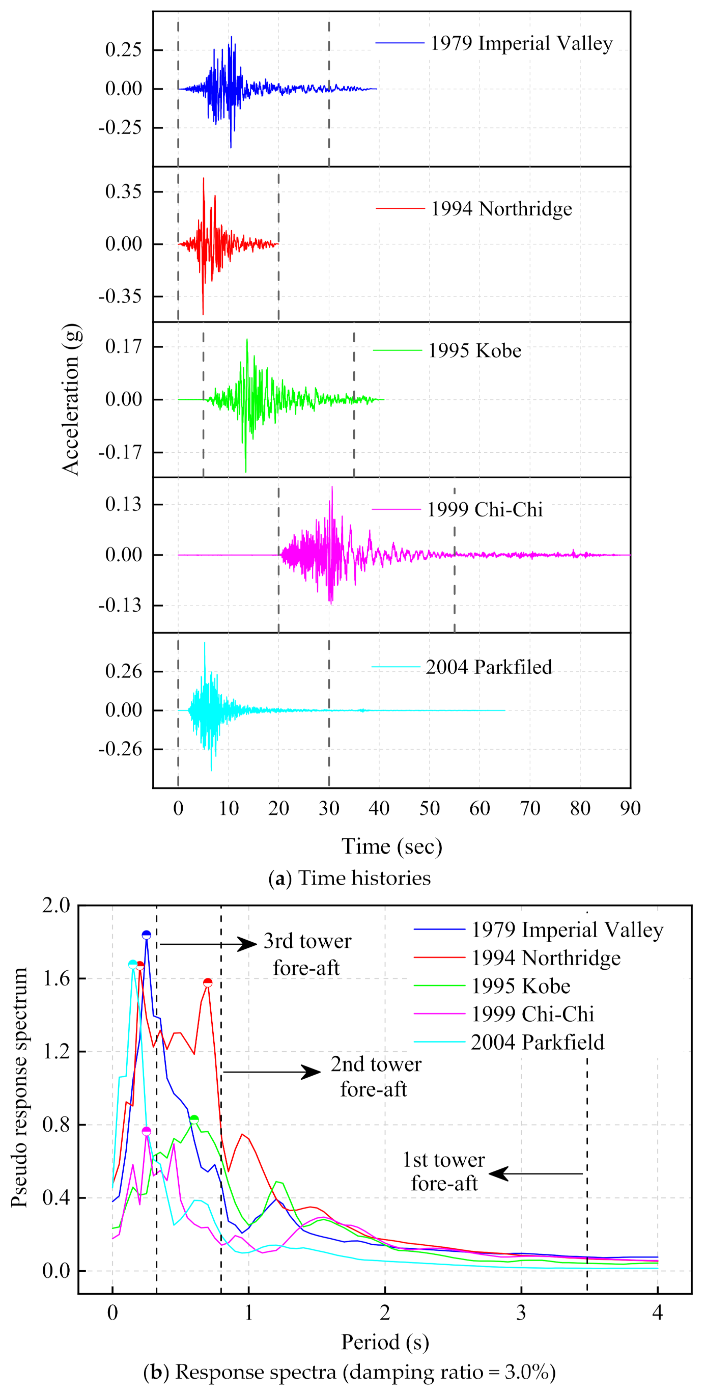
3.4. Earthquake Loading

The medium sand is considered to reproduce the liquefaction phenomenon, and its corresponding shear wave velocity is 198.7 m/s, which corresponds to the Site Class D that is defined in the ASCE 7-10 [97]. Therefore, five earthquake records with a wide range of frequency contents for Site Class D, which is denoted as E1 to E5, are selected, with their PGAs ranging from 0.18 to 0.48 g. Table 3 presents the details of the selected strong ground motion records. Their PGAs are linearly scaled to 0.15 g to meet the requirement for the seismic precautionary intensity level of 7 that is defined in GB 50010-2010 in China [98]. The dominant horizontal components of the strong motion records are inputted to the FE model in this study, and the corresponding acceleration time histories are shown in Figure 6a. It is important to note that only partial records between the dashed grey lines were selected for the dynamic analysis, considering the computation cost. Figure 6b depicts the acceleration response spectra for a damping ratio of 3.0%, wherein the damping ratio corresponds to an operating condition of the OWT. The response spectra for the damping ratio (i.e., 1.5%) in a parked state are not shown herein. All the peak frequencies of the five response spectra are considerably higher than the tower’s first fore–aft frequency, but they are closer to the second or third fore–art frequencies of the tower. In particular, the Northridge earthquake shows two peaks that are close to the second and third fore–art frequencies.

3.5. Simulated Scenarios

Four different scenarios are simulated, as shown in

Table 4. Simulation scenarios for liquefaction evaluation for the OWT.

Scenario	Analysis Object	Wind Speeds (m/s)	Earthquakes		Turbine States	Remarks
			Records	PGA (g)
Scenario 1	Free-field soil	0.0	E1–E5	0.15	-	Earthquake
Scenario 2	OWT	0.0	E1–E5	0.15	Parked	Earthquake
Scenario 3	OWT	11.4	E1–E5	0.15	In-operation	Earthquake + Wind
Scenario 4	OWT	11.4	E1–E5	0.15	In-operation	Earthquake + Wind + Wave

. In Scenario 1, only the soil domain under the selected seismic records is simulated; whereas in Scenario 2, the soil domain plus the OWT superstructure are simulated under the same seismic records. Furthermore, in Scenario 3, the dynamic wind loading corresponding to the rated wind speed is further introduced to simulate the coupled effect of the wind and earthquake loadings on the OWT. The wave load is supplemented in Scenario 4. The simulation time is 5 s beyond the ground motion records in order to consider the dissipation time.

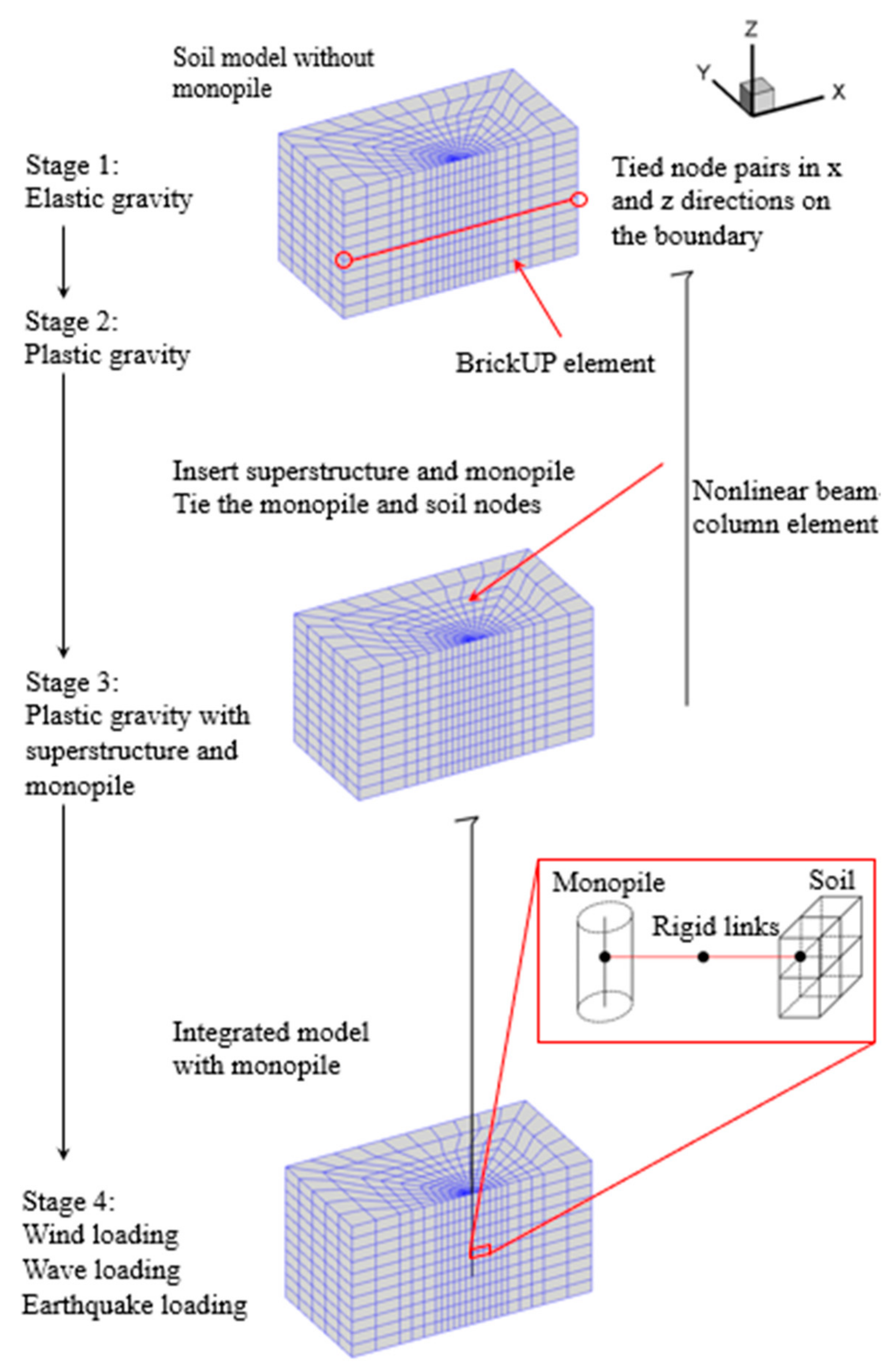
3.6. Staged Simulation Procedure

A staged modeling procedure is employed to simulate the pile existence and to generate accurate initial conditions for the liquefaction assessment [79]. In the first stage, the soil domain without the pile is modeled by adopting the BrickUP elements, with a significant permeability coefficient and a tied boundary condition. An elastic gravity stage is initially carried out. Then, the state of soil is updated by using the proposed plastic model to produce the initial effective stress in Scenario 1. Next, the superstructure, the monopile foundation, and the links are introduced, and three translational DOFs of the monopile and link nodes are tied to adjacent soil nodes. Another plastic gravity step is conducted to account for the settlement and consolidation of the soil that is caused by the pile and the WT gravity, and to generate the proper initial stress for the liquefaction evaluation in Scenarios 2, 3, and 4. After the gravity stages, the earthquake loading or the coupled loadings are applied. The soil permeability coefficient is updated with the appropriate value to simulate the undrained condition of the soil domain. Figure 7 depicts the detailed procedure for Scenarios 2, 3, and 4.

4. Numerical Results and Discussions

The pore water pressure is monitored at seven columns of the soil points, including at SP1×, SP2×, SP3×, SP4×, and SP5× on the left side (upwind) of the monopile, and SP6× and SP7× on the right side (downwind) of the monopile, in order to assess the liquefaction possibility of the soil domain. The “×” symbol represents the numbers, 1–5, for the different soil layers in a column. The vertical displacements at Points DV1 and DV2 are monitored to evaluate the soil settlement and the monopile tilt. The acceleration and displacement at the tower top are also observed, and are denoted as AT and DT, respectively, in order to examine the dynamic responses of the OWT system. Figure 8 shows the detailed layout of the monitoring points.

Table 5. Dynamic response and liquefaction distribution under different simulation scenarios.

Loading Cases		Tower	Pile		Soil
		Tower Top Displacement (m)	Rotation at Mudline (°)	Max Bending Moment (MN-m)	Liquefied Depth (m)	Max EPP 1 (kPa)
						Z = −5 m	Z = −10 m	Z = −15 m
Scenario 1 (S1)	E1	-	-	-	5	44.7	52.5	47.6
	E2	-	-	-	5	44.4	54.2	57.3
	E3	-	-	-	10	44.8	88.3	87.0
	E4	-	-	-	5	44.5	57.1	51.1
	E5	-	-	-	0	33.5	22.6	16.4
Scenario 2 (S2)	E1	0.114	0.065	418.3	10	64.1	90.5	105.7
	E2	0.105	0.097	492.3	10	60.0	90.5	123.8
	E3	0.221	0.145	724.6	15	59.2	102.0	141.6
	E4	0.309	0.092	430.9	10	59.3	91.2	120.5
	E5	0.017	0.035	279.9	5	52.8	52.4	38.2
Scenario 3 (S3)	E1	1.135	0.126	808.9	10	67.6	96.0	102.0
	E2	1.167	0.158	777.6	10	68.5	93.1	117.4
	E3	1.317	0.210	1003.5	15	65.3	108.6	153.6
	E4	1.117	0.143	663.8	10	67.8	90.4	102.0
	E5	1.116	0.095	638.7	5	50.0	55.8	34.4
Scenario 4 (S4)	E1	1.138	0.123	760.3	10	67.2	89.9	112.9
	E2	1.206	0.160	711.5	10	66.6	98.5	105.3
	E3	1.392	0.226	1052.8	15	46.9	107.4	149.6
	E4	1.142	0.130	716.8	10	72.6	91.5	97.6
	E5	1.142	0.087	627.3	5	50.5	60.0	32.5

¹ The monitored soil points are located at X = −7.5 m and Y = 0.0 m.

summarizes the major results that are obtained in the dynamic responses in four simulated loading scenarios. The tower top displacement is examined to guarantee the stable levels and the normal operations of the components (e.g., gearbox, generator, and other equipment) in the nacelle. The pile rotation angle at the mudline shows the inclination of the OWT in the service. The pile bending moment below the mudline is also examined because this index is sensitive to the loading variation that is transferred from the WT system and the liquefaction developed in the surrounding soil domain. Moreover, the moments can also be employed to evaluate the foundation-bearing capacity. Finally, the EPP, which is defined as the difference between the instantaneous pore water pressure and the hydrostatic pore pressure, at the monitoring points, SP11, SP12, and SP13 (on the left side of the monopile), is presented to illustrate the EPP accumulation and to assess the liquefaction distribution.

As the dynamic responses and liquefaction development under five selected earthquake records follow similar trends, the following subsections mainly focus on the Kobe earthquake to explain the dynamic responses and liquefaction potential. This event causes the most severe liquefaction distribution and capacity deterioration.

4.1. The Effect of Seismic Loading Direction

With the introduction of aerodynamic damping, the fore–aft and side–side damping ratios of the operating OWT system are different. Therefore, two cases that represent different input directions for the Kobe (E3) earthquake are considered in Scenario 3 in order to clarify the influence of the angle between the wind and earthquake loadings, and to select the severest liquefaction case in the following simulation. The detailed layouts of the two cases are shown in Figure 9. Considering the asymmetrical characteristics of loading when changing the earthquake incident directions, the full model, instead of the half model, is simulated.

The dynamic response and liquefaction severity are summarized in

Table 6. Dynamic response and liquefaction distribution, with and without considering aerodynamic damping.

Loading Cases		Direction	Tower	Pile
			Tower Top Displacement (m)	Rotation at Mudline (°)	Max Bending Moment (MN-m)
Scenario 3 (S3)	Case 1 1	X	1.302	0.209	1019.3
		Y	0.000	0.000	0.0
	Case 2 2	X	1.206	0.112	525.4
		Y	0.236	0.098	798.2

¹ Wind and earthquake loading directions along the X axis; ² wind and earthquake loading directions along the X and Y axes, respectively.

. In Case 1, the tower top displacement, the rotation angle, and the maximum bending moment in the Y direction are nearly zero, as both the wind and earthquake loadings are applied in the X direction. In Case 2, the dynamic responses in the Y direction intensify with the introduction of the earthquake in this direction. However, the maximum dynamic responses in Table 6 indicate that Case 1, with the consistent wind and earthquake direction, represents the severest situation. Therefore, the discussions in the following subsections are mainly focused on this most critical case. Comparing the results of the half model (shown in Table 5) and the full model (shown in Table 6), Case 1 verifies the accuracy of the half model when the wind and earthquake loading are applied in the same direction.

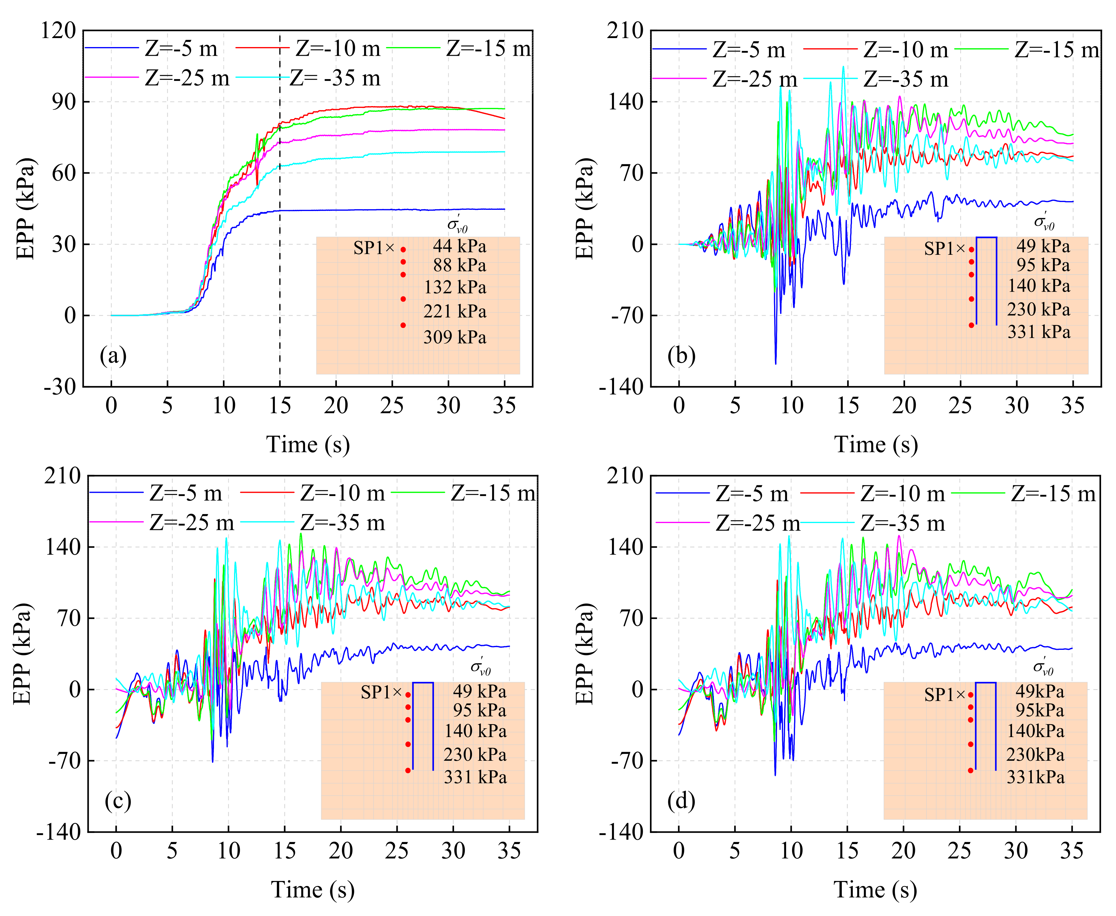
4.2. Liquefaction Analysis of Free-Field Soil (Scenario 1)

As mentioned before, three different mesh sizes (2.5, 5.0, and 10.0 m) are considered horizontally, while a single mesh size of 5.0 m is adopted in the vertical direction. To eliminate the uncertainty that is caused by the mesh sizes, a finer model, which adopts the half values of the mesh sizes in three axes under the Kobe earthquake, was evaluated. The EPP comparison of the two models is shown in

Table 7. Maximum EPP values for wind turbines with various fidelity meshes under Kobe earthquake (E3).

Model	EPP 1 (kPa)
	Z = −5 m	Z = −10 m	Z = −15 m	Z = −25 m	Z = −35 m
Coarse mesh	44.8	88.3	87.0	78.3	68.9
Fine mesh	44.2	85.8	85.4	78.3	68.5
Difference (%)	1.2%	2.7%	1.5%	0.5%	0.6%

¹ The EPPs of monitored soil points are located at X = −7.5 m and Y = 0.0 m.

. The difference between the two different fidelity models is relatively small, and the maximum difference could be found at the soil node with a depth of 10.0 m, which is around 2.7%. The relatively coarser model is adopted in the following simulation to improve the computing efficiency.

Figure 10a presents the development of EPPs under the Kobe earthquake in Scenario 1. The EPP values increase dramatically during the first 15 s for all depths, and then generally remain constant in the remaining time. The EPP of the shallow soil nodes accumulates more quickly than those at deep layers because of the amplified soil responses that are observed at a shallow depth. In addition, the water-depth-induced static water pressure that is imposed on the seabed prevents water drainage, which also contributes to the buildup of EPP at shallow layers. The EPP of the top layer (SP11 at Z= −5 m) reaches approximately 44.0 kPa, and the maximum EPP (88.3 kPa) occurs at the depth of Z = −10 m (SP12). The maximum EPP values at other monitoring nodes (SP13, SP14, and SP15) are 87.2, 78.3, and 68.9 kPa, respectively, which generally decrease with the increasing depth.

The liquefaction areas could be judged on the basis of the excess pore water pressure ratio (EPPR) ($r_u$):

$$r_u=\frac{u(z)}{{\sigma }_{v0}^{\prime }(z)},$$

(20)

where $u(z)$ is the EPP at a depth of $z$, and ${\sigma }_{v0}^{\prime }(z)$ is the initial vertical effective stress, which could be determined on the basis of the computation results before the input of the ground motions. The liquefaction takes place when the EPPR $r_u\ge 0.9$. Figure 11a shows the EPPR diagrams in Scenario 1. The liquefaction depth reaches approximately 10 m during the Kobe earthquake. The shallow layer initially transforms into the liquefied state because of the lower effective stress and the more significant dynamic response. In addition, the EPPR (or EPP) of the soil nodes at the same horizontal level keeps constant, which satisfies the response characteristics of the free-field soil model and eliminates the error that is caused by the different mesh sizes that are adopted in the horizontal directions.

Table 5 presents the detailed results in Scenario 1 (i.e., the free-field soil) under five earthquake records. The liquefaction does not occur under the Parkfield (E5) earthquake, but the liquefaction depths reach approximately 5 m under the other seismic ground motions, except for the Kobe earthquake. Among four liquefied cases, the greatest EPP is observed under the Kobe (E3) earthquake, with the maximum EPP of 88.3 kPa at the depth of Z = −10 m. The different liquefaction severities under five ground motion records are attributed to the different intensities and frequency components of the selected earthquakes (Figure 6). Compared with other seismic ground motions, the predominant frequency of the Kobe earthquake is closer to the fundamental frequency (0.9 Hz) of the free-field soil, which intensifies the dynamic responses and, consequently, leads to more severe liquefaction.

4.3. OWT in the Parked Condition (Scenario 2)

The OWT system supported on a large-diameter monopile under earthquakes is simulated in Scenario 2. Figure 10b shows the EPP variation of the soil nodes (SP1×) at different depths under the Kobe (i.e., E3) earthquake. The development history of the EPP exhibits a similar trend, as is shown in the free field. However, the variation amplitude is more significant in Scenario 2 because of the cyclic tension–compression stress that is induced by the monopile motion. In particular, the EPP around the pile toe (i.e., the depth of Z = −35 m) in Figure 10b accumulates more quickly than that in the free field, as shown in Figure 10a. Furthermore, the maximum EPP values are approximately 68.9 and 174.7 kPa in Scenarios 1 and 2, respectively, which indicates greater stress transfer in this zone in Scenario 2.

Figure 11b shows the EPPR distribution under the Kobe earthquake in Scenario 2 when the EPPR of SP13 (Z = −15 m) reaches the maximum value. At the selected instant, the soil inside and outside the pile shows different states. Considering the confinement of the pile wall, the EPPR of the soil inside the monopile (X = 0 m) is smaller than that outside (X = ±7.5 m), and correspondingly, more severe liquefaction can be found outside of the monopile. Figure 12a shows the EPP variation in the horizontal direction at a selected depth of Z = −15 m, which corresponds to the maximum liquefaction depth (Table 5). The EPP variation is apparently affected by the monopile within the distance of 12.5 m from the pile center, whereas the influence becomes limited beyond the distance of 20 m (approximately twice the monopile diameter).

Figure 13 shows the peak positive and negative bending moment distributions along the pile under the Kobe earthquake in Scenario 2. The maximum bending moments are developed at the depth of approximately 10–15 m, which is close to the interface of the liquefiable and nonliquefiable layers. This result is consistent with the observation that is made by Rahmani and Pak [76] on traditional pile foundations. The averaged maximum and minimum bending moments during the Kobe earthquake are 724.6 and −752.8 MN-m, respectively.

In general, the introduction of the large-diameter monopile in Scenario 2 intensifies the liquefaction severity under all five seismic records, as shown in Table 5. For example, the liquefaction occurs under the Parkfield earthquake in Scenario 2, but not in the free-field soil in Scenario 1. Compared with the shallow soil layers (Z = −5 m), the EPP of the soil at deeper positions (Z = −10 m) increases more significantly to reach the liquefied state under three seismic records (E2, E4, and E5). The most severe liquefied state is still observed in the Kobe case, in which the liquefaction depth expands to 15 m.

Table 5 also presents the pile rotation and bending moment in Scenario 2. The largest rotation angles and bending moments are observed under the Kobe earthquake, which is consistent with the liquefaction severity. Figure 14 shows the time histories of the tower top displacement and the pile rotation at the mudline level under the Kobe earthquake. Given that the current IEC standard has not specified the detailed requirement for OWTs when considering the earthquake loading, some general specifications in different design codes are considered as the evaluation criteria, even though these limits are not originally intended for seismic cases. FD 003-2007 [99] specifies a rotation angle limit of 0.17° for WTs, whereas DNV-OS-J101 [96] defines another limit of 0.25° for OWT structures. These rotation angles are specified to meet the visual requirements and to ensure the normal drivetrain operation. GB 50135-2019 [100] defines an upper limit of tower top displacement as 1/75 of the tower height for high-rise structures, which include WT towers, in order to guarantee adequate resistance capacity. These threshold values are set to meet the requirements for the normal serviceability of WTs. Figure 14 depicts the corresponding values. None of these thresholds exceed in Scenario 2, despite the occurrence of soil liquefaction. The residual tower top displacement and residual pile rotation after the Kobe earthquake are equal to −0.035 m and −0.002°, respectively.

4.4. OWT in Operating Condition (Scenarios 3 and 4)

Scenarios 3 and 4 consider the OWT operating at a rated wind speed, when an earthquake occurs with and without the inclusion of the wave loadings, respectively. As shown in Figure 14a, the maximum displacement at the tower top in Scenario 3 reaches 1.317 m, which is 5.9 times the peak value in Scenario 2, but is slightly smaller than the limit required in GB 50135-2019. The maximum value in Scenario 4 is slightly larger, at around 1.392 m. It is noteworthy that turbulent wind loading was applied before the earthquake attacks, and, thus, the initial displacement is not zero in two scenarios. Moreover, Figure 14b shows that the time histories of the pile rotation angle under the Kobe earthquake in Scenarios 3 and 4 have apparently different magnitudes from that of Scenario 2, which is due to the addition of the wind loading. The maximum values under coupling loading are 0.210 and 0.226°, respectively, which exceeds the 0.17° limit that is defined in FD 003-2007 [99], but still satisfies the limit of 0.25° in DNV-OS-J101 [96].

Figure 10c shows the EPP variation at the soil nodes next to the pile wall under the Kobe (E3) earthquake in Scenario 3, wherein the EEP development history shows a trend similar to that in Scenario 2. The time histories of EPPs at different depths in Scenario 4, as shown in Figure 10d, are generally consistent with those in Scenario 3, except for the normal soil node with a depth of 25 m, where the corresponding EPP value is larger because of the introduction of wave loading. Figure 15a directly compares the EPP development histories between Scenarios 2 and 3 at a selected depth of Z = −15 m, which corresponds to the maximum liquefaction depth in these two scenarios. A noticeable difference can be observed between Scenarios 2 and 3 for the soil nodes next to the pile wall (X = −7.5 m). Following the seismic record peak at 8.46 s, the coupling effect of the wind and earthquake loading has a significant influence on the EPP accumulation and leads to a larger value. In the remaining time, the EPP values in Scenario 2 are slightly greater. The effect of the wave loading on the EPP accumulation is relatively limited when comparing the EPP values in Scenarios 3 and 4, as shown in Figure 15b. The EPPR distributions in Scenarios 3 and 4 when the EPPR of SP13 (Z = −15 m) reaches the maximum are shown in Figure 11c,d, and similar liquefaction distributions could be found.

Figure 13 shows the bending moment distributions along the pile under the Kobe earthquake in Scenarios 3 and 4. The maximum positive bending moments are equal to 1003.5 and 1052.8 MN-m, respectively, in Scenarios 3 and 4; while the minimum values are −494.5 and −430.8 MN-m, respectively. The maximum bending moment increases slightly when the wave loading is included. In comparison to Scenario 2, although the maximum negative bending moment becomes smaller in Scenarios 3 and 4, the maximum positive bending moment, which is regarded as a dominant component, is significantly amplified under the coupled loadings.

Figure 16 directly compares the peak values of several key indices among four scenarios, including the EPP of shallow soil nodes, and the maximum bending moments and rotation angles of the monopile. As shown in Figure 16a, the EPP values in the free-field soil are very close under five earthquakes, except for the Kobe earthquake (E3); whereas the introduction of the OWT and monopile in Scenario 2 will considerably increase the EPP values by 15.5–132.1%. The maximum increment ratio of 132.1% occurs in the Parkfield earthquake (E5) when the liquefaction phenomenon appears with the introduction of the OWT. The further addition of wind loading in Scenario 3 only increases the EPP values slightly (<7%), compared to that in Scenario 2. The influence of the wave loading on the EPP variation in Scenario 4 is not consistent. The EPP values slightly increase in the Northbridge, Chi-Chi, and Parkfield earthquakes (E2, E4, and E5), whereas the smaller EPPs could be found in the other two seismic records.

However, the effects of the coupled earthquake and wind loadings (Scenario 3) become more evident in the pile rotation angles and bending moments, respectively, as shown in Figure 16b,c. The increment ratios range from 38.5 to 128.2% under the coupled earthquake and wind loadings for the maximum bending moment, and the increment ratios of the pile rotation angle at the mudline range from 44.8 to 171.4%. The liquefaction severity has a significant impact on the bending moments and rotation angles of the monopile. Given that the liquefaction depth is only 5 m under the Parkfield (E5) earthquake, the bending moment and rotation angle are relatively small. By contrast, with the largest liquefaction depth under the Kobe (E3) earthquake, the bending moment and rotation angles are maxima among the five earthquake cases. The significant liquefaction weakens the stiffness and capacity of the soil foundation, and thereby amplifies the dynamic responses of the monopile and superstructure. When including the wave loading in Scenario 4, the rotation angle and bending moment are not increased, except for the Kobe earthquake, which corresponds to the severest liquefaction condition. The increment ratios of the rotation angle and the maximum bending moment under the Kobe earthquake are 7.5 and 4.9%, respectively.

Figure 17 depicts the shear stress–shear strain and shear stress–mean effective stress relationships of soil nodes at two selected depths in Scenarios 3. The soil node at a depth of 10 m experiences the maximum shear stress amplitude of 107.06 kPa and the maximum shear strain of 1.906% in Scenario 3, as shown in Figure 17a. The corresponding values in Scenario 2 are only 69.88 kPa and 1.853%, respectively, which are not shown in this paper for brevity. The relatively larger shear stress amplitude and accumulated strain under the coupled loading intensify the soil performance deterioration in Scenario 3. Figure 17b also indicates that the mean effective stress gradually reduces to zero with the loading cycles during the earthquake, which indicates the liquefaction process. In comparison to a 10 m depth, although the soil node at a 25 m depth in Figure 17c experiences larger shear stress, the node is not finally liquefied given the positive mean effective stress.

A similar stress path could be found in Scenario 4 considering the wave loading, but the corresponding shear stress amplitude (104.44 kPa) and maximum shear strain (1.904%) at shallow depth (Z = −10 m) are smaller than those in Scenario 3. For the sake of brevity, the diagrams for Scenario 4 are not shown in Figure 17.

5. Conclusions

On the basis of a three-dimensional FE model of a 10 MW OWT with a large-diameter monopile, the impact of the earthquake-induced seabed liquefaction on a large-scale OWT is systematically assessed in the current study. The solid–fluid fully coupled element, which is based on Biot’s theory for a porous medium, and the pressure-dependent elastoplastic model, are employed to assess the soil displacement and the pore water pressure. Five representative earthquake records are selected to evaluate the dynamic responses of the OWT under combined wind, wave, and earthquake loadings. The major findings are summarized as follows:

(1)

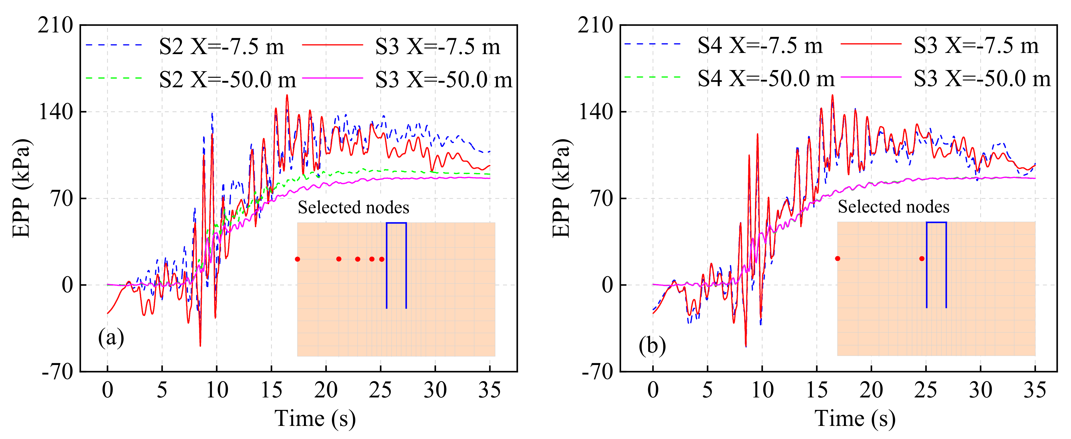
Compared with free-field soil, the large-diameter monopile considerably increases the EPP of the soil surrounding the pile, particularly at the pile toe. However, the influence of the pile becomes limited for soil domain with a horizontal plan distance that is beyond twice the pile diameter;

(2)

The motions of the OWT under earthquake loadings increase the liquefaction depth and intensify the liquefaction severity;

(3)

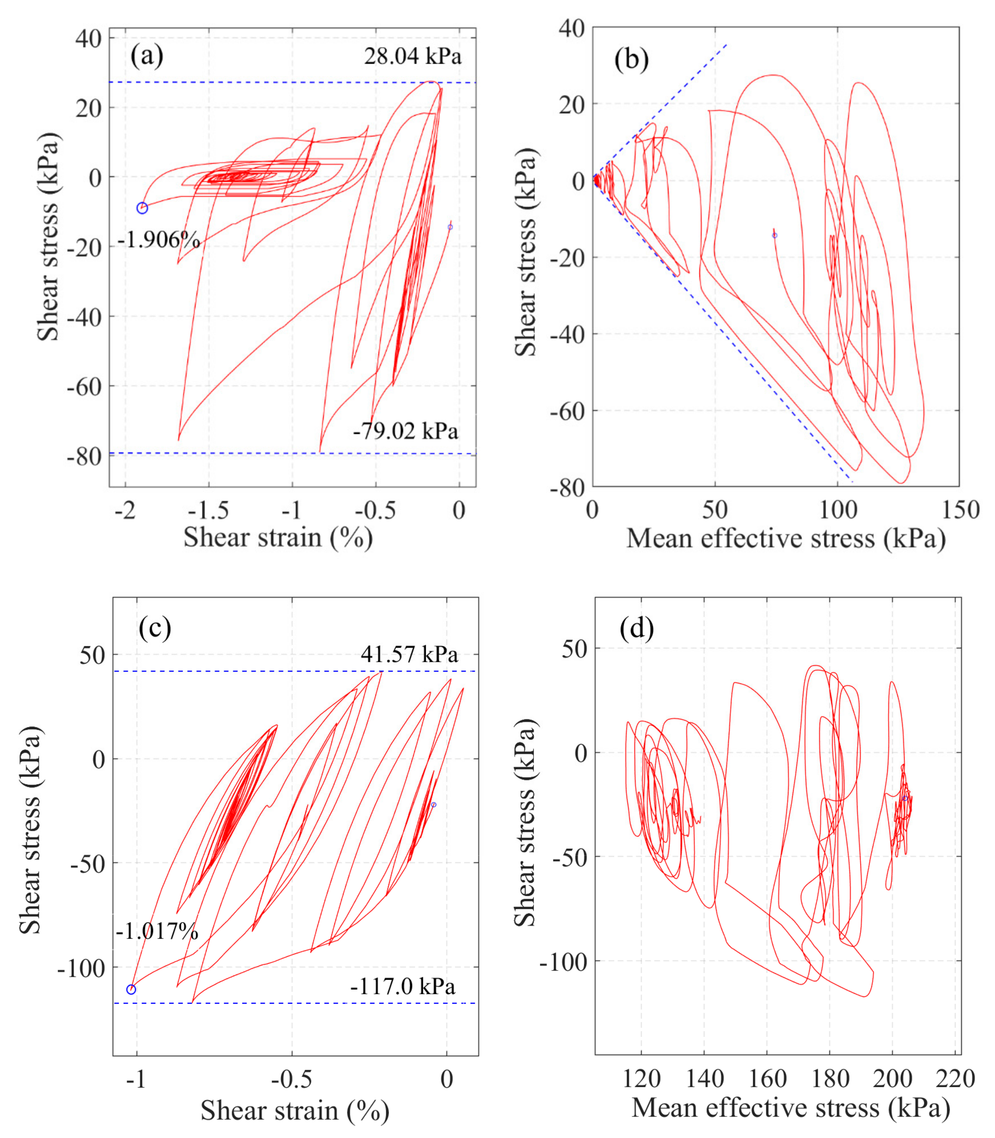
Compared with earthquake loadings, the coupled wind and earthquake loadings have small effects on the EPP values of the soil. However, the introduction of wind loading leads to an increased shear stress amplitude and accumulated shear strain, which has a critical influence on the soil degradation;

(4)

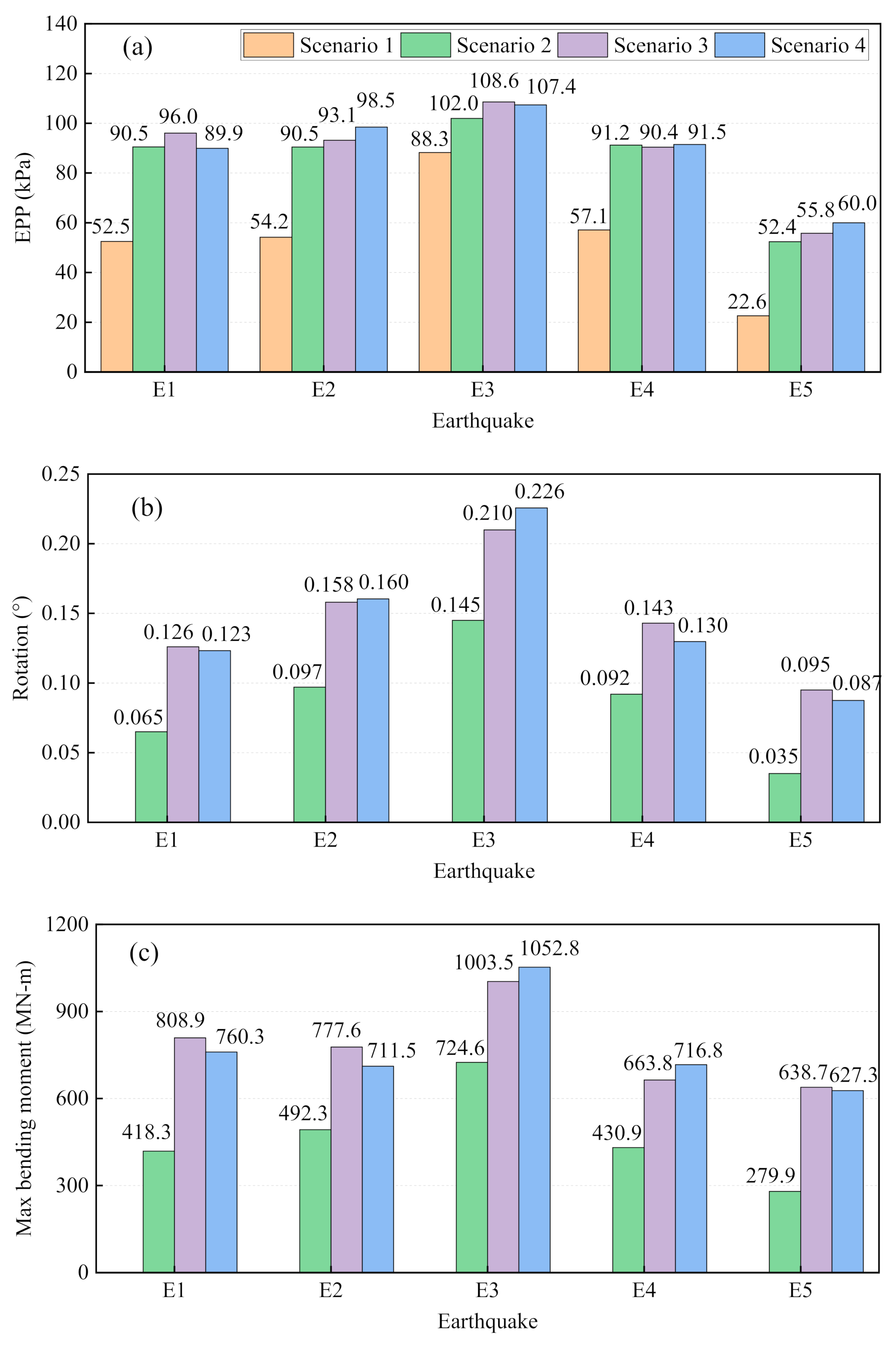
The liquefaction reduces the foundation stiffness and capacity of the OWT. Consequently, under the coupled wind and earthquake loadings, the pile rotation angles at the mudline and tower top displacements increase distinctly. In particular, the maximum pile rotation angle exceeds the limit that is specified in a Chinese standard;

(5)

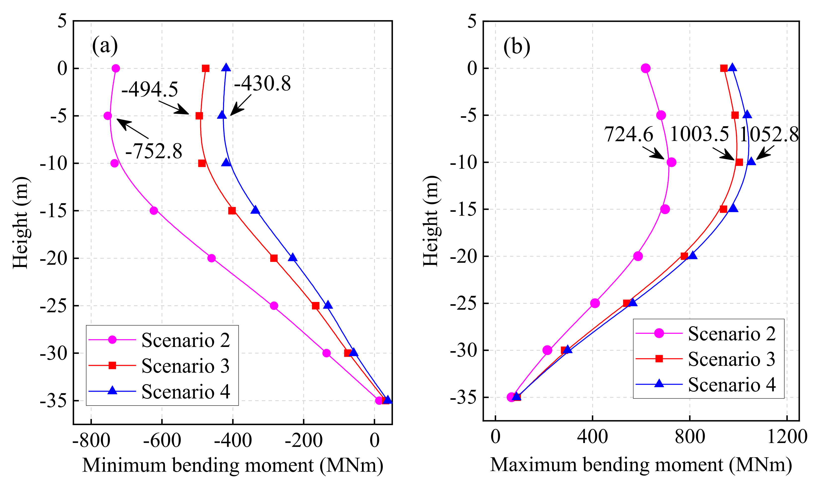
A considerably larger bending moment in the monopile is observed under the coupled wind and earthquake loadings. The peak bending moment occurs with the liquefaction, with the maximum value appearing close to the interface between the liquefiable and nonliquefiable soil layers;

(6)

The influence of the wave loading on the dynamic response (tower top displacement, pile rotation angle, and bending moment) and the liquefaction severity is limited;

(7)

The strong coupling effect between the wind and earthquake loadings indicates that the past seismic analyses of OWTs that overlooked the liquefaction effect have considerably underestimated the seismic risks of OWTs.

On the basis of the dynamic analyses of OWTs on the liquefiable seabed presented in this paper, more systematical future studies will be needed on the following aspects: (1) More load combinations should be analyzed in order to investigate the coupling effect of different loads on the dynamic response of OWTs; and (2) Parametric studies should be carried out to determine the critical factors that control the liquefaction behavior, and, thereby, more effective and practical solutions can be suggested.

References

1. Lee, J.; Zhao, F. Global Wind Energy Council Home Page. Available online: https://gwec.net/global-wind-report-2019/ (accessed on 19 March 2022).
2. Watson, S.; Moro, A.; Reis, V.; Baniotopoulos, C.; Barth, S.; Bartoli, G.; Bauer, F.; Boelman, E.; Bosse, D.; Cherubini, A.; et al. Future emerging technologies in the wind power sector: A European perspective. Renew. Sust. Energy Rev. 2019, 113, 109270. [Google Scholar] [CrossRef]
3. Bento, N.; Fontes, M. Emergence of floating offshore wind energy: Technology and industry. Renew. Sust. Energy Rev. 2019, 99, 66–82. [Google Scholar] [CrossRef]
4. Katsanos, E.I.; Thöns, S.; Georgakis, C.Τ. Wind turbines and seismic hazard: A state-of-the-art review. Wind Energy 2016, 19, 2113–2133. [Google Scholar] [CrossRef] [Green Version]
5. Kaynia, A.M. Seismic considerations in design of offshore wind turbines. Soil Dyn. Earthq. Eng. 2019, 124, 399–407. [Google Scholar] [CrossRef]
6. Veers, P.; Dykes, K.; Lantz, E.; Barth, S.; Bottasso, C.L.; Carlson, O.; Clifton, A.; Green, J.; Green, P.; Holttinen, H.; et al. Grand challenges in the science of wind energy. Science 2019, 366, 443. [Google Scholar] [CrossRef] [PubMed] [Green Version]
7. Skopljak, N. GE Haliade-X 12MW Produces First Power in Rotterdam. Available online: https://www.offshorewind.biz/2019/11/07/ge-haliade-x-12mw-produces-first-power-in-rotterdam/ (accessed on 19 March 2022).
8. Oh, K.; Nam, W.; Ryu, M.S.; Kim, J.; Epureanu, B.I. A review of foundations of offshore wind energy convertors: Current status and future perspectives. Renew. Sust. Energy Rev. 2018, 88, 16–36. [Google Scholar] [CrossRef]
9. Igwemezie, V.; Mehmanparast, A.; Kolios, A. Current trend in offshore wind energy sector and material requirements for fatigue resistance improvement in large wind turbine support structures—A review. Renew. Sust. Energy Rev. 2019, 101, 181–196. [Google Scholar] [CrossRef] [Green Version]
10. Wang, X.; Zeng, X.; Li, J.; Yang, X.; Wang, H. A review on recent advancements of substructures for offshore wind turbines. Energy Convers. Manag. 2018, 158, 103–119. [Google Scholar] [CrossRef]
11. Wu, X.; Hu, Y.; Li, Y.; Yang, J.; Duan, L.; Wang, T.; Adcock, T.; Jiang, Z.; Gao, Z.; Lin, Z.; et al. Foundations of offshore wind turbines: A review. Renew. Sust. Energy Rev. 2019, 104, 379–393. [Google Scholar] [CrossRef] [Green Version]
12. Negro, V.; LópezGutiérrez, J.; Esteban, M.D.; Matutano, C. Uncertainties in the design of support structures and foundations for offshore wind turbines. Renew. Energy 2014, 63, 125–132. [Google Scholar] [CrossRef] [Green Version]
13. Wan, Y.; Fan, C.; Dai, Y.; Li, L.; Sun, W.; Zhou, P.; Qu, X. Assessment of the Joint Development Potential of Wave and Wind Energy in the South China Sea. Energies 2018, 11, 398. [Google Scholar] [CrossRef] [Green Version]
14. Li, X.; Chen, S.; Ren, Z.; Lv, Y.; Tong, H.; Wen, Z. Project plan and research progress on key technologies of seismic zoning in sea areas. Prog. Earthq. Sci. 2020, 50, 2–19. [Google Scholar]
15. Yang, Y.; Ye, K.; Li, C.; Michailides, C.; Zhang, W. Dynamic behavior of wind turbines influenced by aerodynamic damping and earthquake intensity. Wind Energy 2018, 21, 303–319. [Google Scholar] [CrossRef]
16. Kjørlaug, R.A.; Kaynia, A.M. Vertical earthquake response of megawatt-sized wind turbine with soil-structure interaction effects. Earthq. Eng. Struct. Dyn. 2015, 44, 2341–2358. [Google Scholar] [CrossRef]
17. Zafeirakos, A.; Gerolymos, N. On the seismic response of under-designed caisson foundations. Bull. Earthq. Eng. 2013, 11, 1337–1372. [Google Scholar] [CrossRef]
18. Patil, A.; Jung, S.; Kwon, O.-S. Structural performance of a parked wind turbine tower subjected to strong ground motions. Eng. Struct. 2016, 120, 92–102. [Google Scholar] [CrossRef]
19. Santangelo, F.; Failla, G.; Santini, A.; Arena, F. Time-domain uncoupled analyses for seismic assessment of land-based wind turbines. Eng. Struct. 2016, 123, 275–299. [Google Scholar] [CrossRef]
20. Huang, S.; Huang, M.; Lyu, Y.; Xiu, L. Effect of sea ice on seismic collapse-resistance performance of wind turbine tower based on a simplified calculation model. Eng. Struct. 2021, 227, 111426. [Google Scholar] [CrossRef]
21. Alati, N.; Failla, G.; Arena, F. Seismic analysis of offshore wind turbines on bottom-fixed support structures. Philos. Trans. A Math. Phys. Eng. Sci. 2015, 373, 20140086. [Google Scholar] [CrossRef]
22. Santangelo, F.; Failla, G.; Arena, F.; Ruzzo, C. On time-domain uncoupled analyses for offshore wind turbines under seismic loads. Bull. Earthq. Eng. 2018, 16, 1007–1040. [Google Scholar] [CrossRef]
23. Sigurᶞsson, G.Ö.; Rupakhety, R.; Rahimi, S.E.; Olafsson, S. Effect of pulse-like near-fault ground motions on utility-scale land-based wind turbines. Bull. Earthq. Eng. 2020, 18, 953–968. [Google Scholar] [CrossRef]
24. Asareh, M.; Schonberg, W.; Volz, J. Fragility analysis of a 5-MW NREL wind turbine considering aero-elastic and seismic interaction using finite element method. Finite Elem. Anal. Des. 2016, 120, 57–67. [Google Scholar] [CrossRef]
25. Fan, J.; Li, Q.; Zhang, Y. Collapse analysis of wind turbine tower under the coupled effects of wind and near-field earthquake. Wind Energy 2019, 22, 407–419. [Google Scholar] [CrossRef]
26. Kim, D.H.; Lee, S.G.; Lee, I.K. Seismic fragility analysis of 5 MW offshore wind turbine. Renew. Energy 2014, 65, 250–256. [Google Scholar] [CrossRef]
27. Martín del Campo, J.O.; Pozos-Estrada, A. Multi-hazard fragility analysis for a wind turbine support structure: An application to the Southwest of Mexico. Eng. Struct. 2020, 209, 109929. [Google Scholar] [CrossRef]
28. Quilligan, A.; O’Connor, A.; Pakrashi, V. Fragility analysis of steel and concrete wind turbine towers. Eng. Struct. 2012, 36, 270–282. [Google Scholar] [CrossRef]
29. Yang, Y.; Bashir, M.; Li, C.; Wang, J. Analysis of seismic behaviour of an offshore wind turbine with a flexible foundation. Ocean Eng. 2019, 178, 215–228. [Google Scholar] [CrossRef]
30. Yang, Y.; Li, C.; Bashir, M.; Wang, J.; Yang, C. Investigation on the sensitivity of flexible foundation models of an offshore wind turbine under earthquake loadings. Eng. Struct. 2019, 183, 756–769. [Google Scholar] [CrossRef]
31. Zuo, H.; Bi, K.; Hao, H.; Li, C. Influence of earthquake ground motion modelling on the dynamic responses of offshore wind turbines. Soil Dyn. Earthq. Eng. 2019, 121, 151–167. [Google Scholar] [CrossRef]
32. Damgaard, M.; Zania, V.; Andersen, L.V.; Ibsen, L.B. Effects of soil–structure interaction on real time dynamic response of offshore wind turbines on monopiles. Eng. Struct. 2014, 75, 388–401. [Google Scholar] [CrossRef]
33. Wang, P.; Zhao, M.; Du, X.; Liu, J.; Xu, C. Wind, wave and earthquake responses of offshore wind turbine on monopile foundation in clay. Soil Dyn. Earthq. Eng. 2018, 113, 47–57. [Google Scholar] [CrossRef]
34. Wang, P.; Xu, Y.; Zhang, X.; Xi, R.; Du, X. A substructure method for seismic responses of offshore wind turbine considering nonlinear pile-soil dynamic interaction. Soil Dyn. Earthq. Eng. 2021, 144, 106684. [Google Scholar] [CrossRef]
35. Prowell, I.; Veers, P. Assessment of Wind Turbine Seismic Risk: Existing Literature and Simple Study of Tower Moment Demand; Sandia National Laboratories: Albuquerque, NM, USA; Livermore, CA, USA, 2009. [Google Scholar]
36. Wang, Y.; Chai, J.; Chang, Y.; Huang, T.; Kuo, Y. Development of Seismic Demand for Chang-Bin Offshore Wind Farm in Taiwan Strait. Energies 2016, 9, 1036. [Google Scholar] [CrossRef] [Green Version]
37. Kuo, Y.; Chong, K.; Tseng, Y.; Hsu, C.; Lin, C. Assessment on liquefaction potential of seabed soil in Chang-Bin Offshore wind farm considering parametric uncertainty of standard penetration tests. Eng. Geol. 2020, 267, 105497. [Google Scholar] [CrossRef]
38. Xiang, N.; Goto, Y.; Obata, M.; Alam, M.S. Passive seismic unseating prevention strategies implemented in highway bridges: A state-of-the-art review. Eng. Struct. 2019, 194, 77–93. [Google Scholar] [CrossRef]
39. Sumer, B.M.; Ansal, A.; Cetin, K.O.; Damgaard, J.; Gunbak, A.R.; Hansen, N.-E.O.; Sawicki, A.; Synolakis, C.E.; Yalciner, A.C.; Yuksel, Y.; et al. Earthquake-Induced Liquefaction around Marine Structures. J. Waterw. Port Coast. Ocean Eng. 2007, 133, 55–82. [Google Scholar] [CrossRef]
40. Barari, A.; Bagheri, M.; Rouainia, M.; Ibsen, L.B. Deformation mechanisms for offshore monopile foundations accounting for cyclic mobility effects. Soil Dyn. Earthq. Eng. 2017, 97, 439–453. [Google Scholar] [CrossRef] [Green Version]
41. Patra, S.K.; Haldar, S. Response of monopile supported offshore wind turbine in liquefied soil. In Proceedings of the Indian Geotechnical Conference, Bengaluru, India, 13–15 December 2018; pp. 1–8. [Google Scholar]
42. Patra, S.K.; Haldar, S. Fore-aft and the side-to-side response of monopile supported offshore wind turbine in liquefiable soil. Mar. Georesour. Geotechnol. 2021, 39, 1411–1432. [Google Scholar] [CrossRef]
43. Patra, S.K.; Haldar, S. Seismic response of monopile supported offshore wind turbine in liquefiable soil. Structures 2021, 31, 248–265. [Google Scholar] [CrossRef]
44. Kementzetzidis, E.; Corciulo, S.; Versteijlen, W.G.; Pisanò, F. Geotechnical aspects of offshore wind turbine dynamics from 3D non-linear soil-structure simulations. Soil Dyn. Earthq. Eng. 2019, 120, 181–199. [Google Scholar] [CrossRef]
45. Zhang, P.; Xiong, K.; Ding, H.; Le, C. Anti-liquefaction characteristics of composite bucket foundations for offshore wind turbines. J. Renew. Sustain. Energy 2014, 6, 053102. [Google Scholar] [CrossRef]
46. Zhang, P.; Ding, H.; Le, C. Seismic response of large-scale prestressed concrete bucket foundation for offshore wind turbines. J. Renew. Sustain. Energy 2014, 6, 013127. [Google Scholar] [CrossRef]
47. Seed, H.B.; Idriss, I.M. A Simplified Procedure for Evaluating Soil Liquefaction Potential; University of California: Berkeley, CA, USA, 1970. [Google Scholar]
48. Shanon and Wilson Inc. Evaluation of Soil Liquefaction Potential for Level Ground during Earthquakes; Shannon & Wilson, Inc. and Agbabian Associates: Seattle, WA, USA; El Segundo, CA, USA, 1976. [Google Scholar]
49. Gao, B.; Ye, G.; Zhang, Q.; Xie, Y.; Yan, B. Numerical simulation of suction bucket foundation response located in liquefiable sand under earthquakes. Ocean Eng. 2021, 235, 109394. [Google Scholar] [CrossRef]
50. Esfeh, P.K.; Kaynia, A.M. Numerical modeling of liquefaction and its impact on anchor piles for floating offshore structures. Soil Dyn. Earthq. Eng. 2019, 127, 105839. [Google Scholar] [CrossRef]
51. Esfeh, P.K.; Kaynia, A.M. Earthquake response of monopiles and caissons for Offshore Wind Turbines founded in liquefiable soil. Soil Dyn. Earthq. Eng. 2020, 136, 106213. [Google Scholar] [CrossRef]
52. Esfeh, P.K.; Govoni, L.; Kaynia, A.M. Seismic response of subsea structures on caissons and mudmats due to liquefaction. Mar. Struct. 2021, 78, 102972. [Google Scholar] [CrossRef]
53. Tsiapas, Y.Z.; Chaloulos, Y.K.; Bouckovalas, G.D.; Bazaios, K.N. Performance based design of Tension Leg Platforms under seismic loading and seabed liquefaction: A feasibility study. Soil Dyn. Earthq. Eng. 2021, 150, 106894. [Google Scholar] [CrossRef]
54. Chaloulos, Y.K.; Tsiapas, Y.Z.; Bouckovalas, G.D. Seismic analysis of a model tension leg supported wind turbine under seabed liquefaction. Ocean Eng. 2021, 238, 109706. [Google Scholar] [CrossRef]
55. Fard, M.M.; Erken, A.; Erkmen, B.; Ansal, A. Analysis of Offshore Wind Turbine by considering Soil-Pile-Structure Interaction: Effects of Foundation and Sea-Wave Properties. J. Earthquake Eng. 2021, 1–23. [Google Scholar] [CrossRef]
56. Li, X.; Zeng, X.; Yu, X.; Wang, X. Seismic response of a novel hybrid foundation for offshore wind turbine by geotechnical centrifuge modeling. Renew. Energy 2021, 172, 1404–1416. [Google Scholar] [CrossRef]
57. Wang, X.; Yang, X.; Zeng, X. Seismic centrifuge modelling of suction bucket foundation for offshore wind turbine. Renew. Energy 2017, 114, 1013–1022. [Google Scholar] [CrossRef]
58. Wang, X.; Zeng, X.; Li, X.; Li, J. Liquefaction characteristics of offshore wind turbine with hybrid monopile foundation via centrifuge modelling. Renew. Energy 2020, 145, 2358–2372. [Google Scholar] [CrossRef]
59. Ko, Y.-Y.; Li, Y.-T.; Chen, C.-H.; Yeh, S.-Y.; Hsu, S.-Y. Influences of repeated liquefaction and pulse-like ground motion on the seismic response of liquefiable ground observed in shaking table tests. Eng. Geol. 2021, 291, 106234. [Google Scholar] [CrossRef]
60. Ko, Y.Y.; Li, Y.T. Response of a scale-model pile group for a jacket foundation of an offshore wind turbine in liquefiable ground during shaking table tests. Earthq. Eng. Struct. Dyn. 2020, 49, 1682–1701. [Google Scholar] [CrossRef]
61. Bak, C.; Zahle, F.; Bitsche, R.; Kim, T.; Yde, A.; Henriksen, L.C.; Natarajan, A.; Hansen, M.H. Description of the DTU 10 MW Reference Wind Turbine; DTU Wind Energy: Roskilde, Denmark, 2013. [Google Scholar]
62. Velarde, J. Design of Monopile Foundations to Support the DTU 10 MW Offshore Wind Turbine. Master’s Thesis, Delft University of Science and Technology and Norwegian University of Science and Technology, Trondheim, Norway, 2016. [Google Scholar]
63. De Risi, R.; Bhattacharya, S.; Goda, K. Seismic performance assessment of monopile-supported offshore wind turbines using unscaled natural earthquake records. Soil Dyn. Earthq. Eng. 2018, 109, 154–172. [Google Scholar] [CrossRef]
64. Dong, R.G. Effective Mass and Damping of Submerged Structures; Lawrence Livermore National Laboratory: Livermore, CA, USA, 1978. [Google Scholar]
65. DNVGL-RP-C205; Environmental Conditions and Environmental Loads. Det Norske Veritas and Germanischer Lloyd: Oslo, Norway, 2017.
66. ISO 19901-4; Petroleum and Natural Gas Industries-Specific Requirements for Offshore Structures Part 4: Geotechnical and Foundation Design Considerations. International Organization for Standardization: Geneva, Switzerland, 2016.
67. DNVGL-RP-C212; Offshore Soil Mechanics and Geotechnical Engineering. Det Norske Veritas and Germanischer Lloyd: Oslo, Norway, 2019.
68. Lu, J.; Elgamal, A.; Yan, L.; Law, K.H.; Conte, J.P. Large-Scale Numerical Modeling in Geotechnical Earthquake Engineering. Int. J. Geomech. 2011, 11, 490–503. [Google Scholar] [CrossRef] [Green Version]
69. Qiu, Z.; Lu, J.; Elgamal, A.; Su, L.; Wang, N.; Almutairi, A. OpenSees Three-Dimensional Computational Modeling of Ground-Structure Systems and Liquefaction Scenarios. Comput. Model. Eng. Sci. 2019, 120, 629–656. [Google Scholar] [CrossRef]
70. Prevost, J.H. Mathematical modelling of monotonic and cyclic undraind clay behavior. Int. J. Numer. Anal. Methods Geomech. 1977, 1, 195–216. [Google Scholar] [CrossRef]
71. Prevost, J.H. A simple plasticity theory for frictional cohesionless soils. Soil Dyn. Earthq. Eng. 1985, 4, 9–17. [Google Scholar] [CrossRef]
72. Zhang, X.; Tang, L.; Ling, X.; Chan, A.H.C.; Lu, J. Using peak ground velocity to characterize the response of soil-pile system in liquefying ground. Eng. Geol. 2018, 240, 62–73. [Google Scholar] [CrossRef]
73. Cheng, Z.; Jeremić, B. Numerical modeling and simulation of pile in liquefiable soil. Soil Dyn. Earthq. Eng. 2009, 29, 1405–1416. [Google Scholar] [CrossRef]
74. Dafalias, Y.F.; Manzari, M.T. Simple Plasticity Sand Model Accounting for Fabric Change Effects. J. Eng. Mech. 2004, 130, 622–634. [Google Scholar] [CrossRef]
75. Manzari, M.T.; Dafalias, Y.F. A critical state two-surface plasticity model for sands. Géotechnique 1997, 47, 255–272. [Google Scholar] [CrossRef]
76. Rahmani, A.; Pak, A. Dynamic behavior of pile foundations under cyclic loading in liquefiable soils. Comput. Geotech. 2012, 40, 114–126. [Google Scholar] [CrossRef]
77. Wilson, D.W. Soil-Pile-Superstructure Interaction in Liquefying Sand and Soft Clay. Ph.D. Thesis, University of California, Davis, CA, USA, 1998. [Google Scholar]
78. Wang, R.; Zhang, J.-M.; Wang, G. A unified plasticity model for large post-liquefaction shear deformation of sand. Comput. Geotech. 2014, 59, 54–66. [Google Scholar] [CrossRef]
79. Wang, R.; Fu, P.; Zhang, J.-M. Finite element model for piles in liquefiable ground. Comput. Geotech. 2016, 72, 1–14. [Google Scholar] [CrossRef] [Green Version]
80. Elgamala, A.; Yang, Z.; Parrab, E. Computational modeling of cyclic mobility and post-liquefaction site response. Soil Dyn. Earthq. Eng. 2002, 22, 259–271. [Google Scholar] [CrossRef]
81. Yang, Z.; Lu, J.; Elgamal, A. OpenSees Soil Models and Solid-Fluid Fully Coupled Elements User’s Manual; University of California: San Diego, CA, USA, 2008. [Google Scholar]
82. Chiaramonte, M.M.; Arduino, P.; Lehman, D.E.; Roeder, C.W. Seismic analyses of conventional and improved marginal wharves. Earthquake Eng. Struct. Dyn. 2013, 42, 1435–1450. [Google Scholar] [CrossRef]
83. Law, H.K.; Lam, I.P. Application of Periodic Boundary for Large Pile Group. J. Geotech. Geoenviron. Eng. 2001, 127, 889–892. [Google Scholar] [CrossRef]
84. Elgamal, A.; Yan, L.; Yang, Z.; Conte, J.P. Three-Dimensional Seismic Response of Humboldt Bay Bridge-Foundation-Ground System. J. Struct. Eng. 2008, 134, 1165–1176. [Google Scholar] [CrossRef] [Green Version]
85. Valamanesh, V.; Myers, A.T. Aerodynamic Damping and Seismic Response of Horizontal Axis Wind Turbine Towers. J. Struct. Eng. 2014, 140, 04014090. [Google Scholar] [CrossRef]
86. Mo, R.; Kang, H.; Li, M.; Zhao, X. Seismic Fragility Analysis of Monopile Offshore Wind Turbines under Different Operational Conditions. Energies 2017, 10, 1037. [Google Scholar] [CrossRef] [Green Version]
87. Zuo, H.; Bi, K.; Hao, H. Dynamic analyses of operating offshore wind turbines including soil-structure interaction. Eng. Struct. 2018, 157, 42–62. [Google Scholar] [CrossRef]
88. Ali, A.; De Risi, R.; Sextos, A.; Goda, K.; Chang, Z. Seismic vulnerability of offshore wind turbines to pulse and non-pulse records. Earthq. Eng. Struct. Dyn. 2019, 49, 24–50. [Google Scholar] [CrossRef]
89. Hudson, M.; Idriss, I.M.; Beikae, M. User’s Manual’s for QUAD4M a Computer Program to Evaluate the Seismic Response of Soil Structures Using Finite Element Procedures and Incorporating a Compliant base; University of California: Davis, CA, USA, 1994. [Google Scholar]
90. IEC 61400-3-1; Wind Energy Generation Systems Part 3-1: Design Requirements for Fixed Offshore Wind Turbines. International Electrotechnical Commission: Geneva, Switzerland, 2019.
91. Jonkman, J.M.; Buhl, M.L. FAST User’s Guide; National Renewable Energy Laboratory (NREL): Golden, CO, USA, 2005. [Google Scholar]
92. Frohboese, P.; Schmuck, C.; Hassan, G.G. Thrust coefficients used for estimation of wake effects for fatigue load calculation. In Proceedings of the European Wind Energy Conference and Exhibition, Warsaw, Poland, 20–23 April 2010. [Google Scholar]
93. Arany, L.; Bhattacharya, S.; Macdonald, J.; Hogan, S.J. Design of monopiles for offshore wind turbines in 10 steps. Soil Dyn. Earthq. Eng. 2017, 92, 126–152. [Google Scholar] [CrossRef] [Green Version]
94. Jonkman, B.J.; Buhl, J.M.L. TurbSim User’s Guide; National Renewable Energy Laboratory (NREL): Golden, CO, USA, 2006. [Google Scholar]
95. Moriarty, P.J.; Hansen, A.C. AeroDyn Theory Manual; National Renewable Energy Laboratory (NREL): Golden, CO, USA, 2005. [Google Scholar]
96. DNV-OS-J101; Design of Offshore Wind Turbine Structures. Det Norske Veritas: Oslo, Denmark, 2014.
97. ASCE/SEI 7-10; Minimum Design Loads for Buildings and Other Structures. American Society of Civil Engineers: Reston, VA, USA, 2010.
98. GB 50011-2010; Code for seismic design of buildings. China Planning Press: Beijing, China, 2016.
99. FD 003-2007; Design regulations on subgrade and foundations for wind turbine generator system. China Water & Power Press: Beijing, China, 2007.
100. GB 50135-2019; Standard for design of high-rising structures. China Planning Press: Beijing, China, 2019.
Figure 1. Development history of total installation of WTs (onshore and offshore) (GWEC 2021).
Energies 15 02539 g001
Figure 2. Wind power and earthquake distribution in the South China Sea: (a) the average wind power density (1979–2016) [13]; and (b) seismic epicenter distribution (BC1767–2018) [14].
Energies 15 02539 g002
Figure 3. Schematic representation of the OWT model and environmental loading.
Energies 15 02539 g003
Figure 4. Constitutive model of PressureDependentMultiYield material [81]: (a) schematic of the constitutive model; and (b) conical yield surfaces in principal stress space and deviatoric plane.
Energies 15 02539 g004
Figure 5. Environment loading: (a) wind loading imposed at the hub; and (b) wave loadings on pile nodes.
Energies 15 02539 g005
Figure 6. Acceleration time histories and response spectra of five selected ground motion records.
Energies 15 02539 g006
Figure 7. Simulation procedure for the OWT system in liquefiable soil.
Energies 15 02539 g007
Figure 8. Monitoring points in dynamic response and liquefaction analysis.
Energies 15 02539 g008
Figure 9. OWT model considering different earhthquake induction directions in Scenario 3: (a) Case 1; and (b) Case 2.
Energies 15 02539 g009
Figure 10. EPPs at different depths (Z) under the Kobe earthquake: (a) Free-field in Scenario 1; (b) WT system in Scenario 2; (c) WT system in Scenario 3; and (d) WT system in Scenario 4.
Energies 15 02539 g010
Figure 11. Liquefaction distribution of the soil domain under the Kobe earthquake: (a) Free-field in Scenario 1; (b) WT system in Scenario 2; (c) WT system in Scenario 3; and (d) WT system in Scenario 4.
Energies 15 02539 g011
Figure 12. EPP of soil nodes with different distances from the pile under Kobe earthquake: (a) EPP accumulation in Scenario 2; (b) EPP accumulation in Scenario 3; and (c) EPP accumulation in Scenario 4.
Energies 15 02539 g012
Figure 13. Bending moment distributions along the monopile under the Kobe earthquake (a) Minimum bending moment; (b) Maximum bending moment.
Energies 15 02539 g013
Figure 14. Tower top displacement and pile rotation under the Kobe earthquake in Scenarios 2–4: (a) tower top displacements; and (b) pile rotation angles at the mudline.
Energies 15 02539 g014
Figure 15. EPP comparison of soil nodes with different distances from the pile under Kobe earthquake in: (a) Scenarios 2 and 3; and (b) Scenarios 3 and 4.
Energies 15 02539 g015
Figure 16. Comparison of various performance indices among four scenarios: (a) EPP of soil node with a depth of 10 m; (b) pile rotation angle at the mudline; and (c) maximum bending moment along the pile.
Energies 15 02539 g016
Figure 17. Shear stress–strain and shear stress–mean effective stress relationships of soil nodes around the piles under Kobe earthquake in Scenario 3: (a) shear stress–strain relationship at Z = −10 m; (b) shear stress–mean effective stress relationship at Z = −10 m; (c) shear stress–strain relationship at Z = −25 m; and (d) shear stress–mean effective stress relationship at Z = −25 m.
Energies 15 02539 g017