Article

Spatial-Temporal Pattern and Driving Factors of Carbon Efficiency in China: Evidence from Panel Data of Urban Governance

1
College of Energy Science and Engineering, Xi’an University of Science and Technology, Xi’an 710054, China
2
Research Center for Energy Economy and Management, Xi’an University of Science and Technology, Xi’an 710054, China
3
China Institute of Urban Governance, Shanghai Jiao Tong University, Shanghai 200030, China
4
China SJTU-UNIDO Joint Institute of Inclusive and Sustainable Industrial Development, Shanghai Jiao Tong University, Shanghai 200030, China
5
School of International and Public Affairs, Shanghai Jiao Tong University, Shanghai 200030, China
6
School of Management, Yan’an University, Yan’an 716000, China
*
Authors to whom correspondence should be addressed.
These authors contributed equally to this work.
Energies 2022, 15(7), 2536; https://doi.org/10.3390/en15072536
Submission received: 7 February 2022 / Revised: 26 March 2022 / Accepted: 28 March 2022 / Published: 30 March 2022
(This article belongs to the Special Issue Advances in CO2 Mitigation in Energy and the Environment)

Abstract

:
The improvement in city-level carbon efficiency (CE) is crucial for China to achieve its CO2 emission targets. Based on the panel data from 2003 to 2017, total factor CE values of 283 prefecture-level cities were measured using the super-efficiency SBM model. Through the exploratory spatial data analysis (ESDA), we found that the average city-level CE from 2003 to 2017 showed a “W”-type growth trend. Additionally, there are significant spatial heterogeneity and spatial dependency characteristics of city-level CE. The results of local spatial correlation analysis showed that the Low–Low clusters are distributed in all cities of Shanxi and Northern Shaanxi, and gradually expand to Inner Mongolia, Gansu, Ningxia, and Hebei over time, and the High–High clusters are mainly located in the southeast coastal cities and central and eastern Sichuan. High–Low clusters are generally scattered in cities with relatively superior political–economic status in Northeast China, North China, and Northwest China, and gradually concentrated in North China during 2003–2017. Additionally, the dynamic spatial econometric model was employed to investigate the influencing factors of CE, and we found that the city-level CE has the characteristic of path dependence on time. Factors such as industrial structure upgrading and environmental regulation have significant improvement effects on city-level CE, while technological progress, financial development, energy intensity, and government intervention can significantly inhibit city-level CE. Compared with short-term effects, the long-term effects are insignificant with higher absolute values, indicating the long-term persistence and gradual strengthening characteristics of driving factors on city-level CE; however, the acting long-term mechanism has not been formed. Additionally, the regional spillover effect of driving factors on CE is more significant in the short term. Based on the empirical results, some policy implications for cities to improve CE are proposed.

1. Introduction

Global warming caused by the continuous growth of greenhouse gas (GHG) emissions has produced many environmental problems that seriously threaten human survival and development. As the world’s largest CO2 emitter since 2006 [1], China has made a commitment to peak CO2 emissions around 2030 and achieve carbon neutrality by 2060. However, China is still the largest developing country in the world. Determining how to break environmental constraints and achieve low-carbon economic development is the key problem that China will face in the future. From the perspective of total factor efficiency, carbon efficiency (CE) can be understood as the degree to which carbon intensity can be reduced under the given input of production factors. Improving CE is an effective way to solve the problem [2,3,4].
With the rapid development of urbanization, cities have become the main source of energy consumption and CO2 emissions in China. The International Energy Agency (IEA) has predicted that China’s urban energy consumption will account for 83% of the national consumption by 2030, generating significant CO2 emissions [5]. Cities play an important role in reducing CO2 emissions [6,7]. However, because of the economic and social connection between regions and pollutant spillover, the spatial spillover effect of CO2 emissions is significant [8,9], and is more obvious with the deepening of regional coordinated development. Therefore, based on the regional perspective and spatial analysis theory, measuring the city-level CE, analyzing spatial characteristics, and exploring the driving factors to formulate differentiated and scientific CO2 emission reduction policies are important issues for China’s cities to realize green economy development.
The research on CE mainly focuses on three aspects. First, the measurement of CE. In previous studies, scholars used a single index to define CE, such as carbon productivity [10], the proportion of CO2 emissions and energy consumption [11], and CO2 emission intensity [12], which only reflect the influence of a single factor on CO2 emissions. A more comprehensive CE index was later proposed [13,14], which considers all relevant indicators of population, energy consumption, economic activity, and CO2 emissions.
It is necessary to establish the production frontier to measure relative efficiency. Data Envelopment Analysis (DEA) and Stochastic Frontier Analysis (SFA) are widely used to establish multiple-input and -output efficiency frontiers and measure efficiency. SFA is a parameter method that mainly measures the effectiveness of efficiency through random error terms. DEA is a nonparametric method with low requirements for data. It does not require model form design [15,16], and is more and more widely used in environmental performance evaluation [17,18,19,20]. The traditional DEA does not consider the unexpected output. Färe et al. [21] first proposed the weak disposability of unexpected output and established nonlinear programming based on unexpected output. However, the solution process is complex and deviates from the actual production process. Subsequently, the directional distance function [22] and the non-radial DEA model, i.e., the Slacks-Based Measure (SBM) model [23], were proposed. For example, the CE values of 30 provinces in China were calculated [24,25]. The total factor CE values of 31 manufacturing industries in China from 2012 to 2016 were calculated based on the improved non-radial distance function [26].
Second, the spatial analysis of CE. Numerous studies have found that CE has significant spatial dependency. Yan et al. [27] used the unexpected output SBM model to calculate the CE of the power sector in 30 provinces in China, and found significant spatial dependency characteristics, especially in the eastern region with a developed economy. Zhu et al. [28] calculated the CE of China’s provincial energy-intensive industries and found that CE has significant spatial heterogeneity and spatial agglomeration characteristics, the most significant in the eastern region. It was found that China’s industrial CE is the highest in the east, the second highest in the middle, and the lowest in the west [29]. Several studies found that there is significant regional heterogeneity in China’s CO2 emission performance [25,30].
Third, the influencing factors of CE. In terms of research methods, previous studies mainly used decomposition methods [31,32] and econometric models [33,34,35]. For example, Zhou et al. [36] constructed the GVAR model of the construction industry and found that technological progress and energy structure adjustment were conducive to improving the CE, while the extensive economic growth mode significantly inhibited the CE. By exploring the Tobit model, Zeng et al. [37] found that industrial structure, external development, and scientific and technological levels were significantly positively correlated with CE, while government intervention and energy intensity were negatively correlated with CE. With the verification of spatial agglomeration characteristics and the spatial spillover effect of environmental pollution [38,39,40], spatial econometric models are widely used. For example, Chu et al. [41] constructed a spatial econometric model and found that there were significant differences in energy mismatch between regions. The impact of energy mismatch on CE in the eastern region was positive, while the impact in the central and western regions was mostly negative. Zhang et al. [42] constructed a spatial lag model and found that China’s carbon productivity has an obvious positive spatial spillover effect. Foreign trade has significantly improved China’s CE, and exports have the most significant effect. On the whole, a large number of studies show that economic development, urbanization, resource endowment, energy structure, technological progress, geographical location, industrial structure, foreign trade, and environmental regulation are the main factors affecting CE [25,28,37,43,44,45].
To summarize, there are some deficiencies and differences in scalability of current research on CE. (1) From the research perspective, the current studies are conducted at a national scale, provincial scale, or industrial scale. There are few studies focusing on city-level CE due to data accessibility. As the main places of production and life, taking cities as units is more conducive to the implementation of emission reduction policies. Therefore, in this paper, we focus on city-level CE. (2) Numerous studies use SBM to measure environmental efficiency, but the values are between 0 and 1, so it is impossible to specifically distinguish the situation where multiple decision-making units are 1 at the same time. Based on the research of Andersen et al. [46], Tone [47] proposed a super-efficiency SBM model, which overcomes the aforementioned flaw and is widely used in environmental efficiency evaluation [48,49,50,51]. Therefore, this paper employs the super-efficiency SBM model to calculate the city-level total factor CE. (3) In terms of analyzing the driving factors of CE with spatial econometric models, previous studies mainly adopt static models, which neglect the inter-temporal effect of environmental pollution and cannot provide a basis for the dynamic law in the temporal and spatial patterns. In addition, few studies consider the role of financial development in environmental efficiency. An increasing number of studies posit that financial development has a key effect on environmental quality, especially the evolution of CO2 emissions [52,53]. According to the research of Chen, Y. (2020), this study assumed SSP2 as a baseline scenario, which can be considered a business-as-usual scenario and maintains historical development features [54]. Referring to the research of Zhou et al. [55], this study defines the carbon efficiency as the ratio of potential carbon intensity to actual carbon intensity within the full factor framework. Therefore, in this paper, we take China’s 283 prefecture-level cities into account and use the super-efficiency SBM model to measure the city-level total factor CE. Then, we employ the exploratory spatial data analysis (ESDA) to explore the spatial–temporal characteristics and construct a dynamic spatial econometric model to explore the driving factors of city-level CE.
The rest of the paper is organized as follows. Section 2 introduces the research methods. Section 3 presents the data sources and variable selection methods. Section 4 presents the results and analysis, including the spatial–temporal characteristics and driving factors of city-level CE. Section 5 provides conclusions and policy recommendations.

2. Methods

2.1. Environmental Production Technology

Environmental production technology is a production possibility set including desirable outputs and undesirable outputs. Assuming that each decision unit invests capital (K), labor (L), and energy (E) in the production process, desirable output (Y) and undesirable output CO2 emissions (C) are produced. The production technology set T can be expressed as:
T = ( K , L , E , Y , C ) : ( K , L , E )   can   produce   ( Y , C )
The production technology set cc: closed sets, bounded sets, strong disposability of inputs and desirable outputs, null-jointness, and weak disposability of desirable and undesirable outputs [22]. Assuming constant returns to scale, environmental production technology set T can be expressed as:
T = ( K , L , E , Y , C ) : n = 1 N Z n K n   K ;   n = 1 N Z n L n   L ;   n = 1 N Z n E n   E ; n = 1 N Z n Y n   Y ;   n = 1 N Z n C n   = C ; Z n 0 , n = 1 , 2 , N
where Zn indicates the intensity variable for constructing the environmental production technology set. Referring to the research of Zhou et al. [55], we construct the following non-radial directional distance function for cities
D ( K , L , E , Y , C ; g ) = sup w T β : ( ( K , L , E , Y , C ) + g · diag ( β ) ) T
where w T = ( w K , w L , w E , w Y , w C ) and g = ( g K , g L , g E , g Y , g C ) indicate the normalized weight vector and explicit directional vector, β = ( β K , β L , β E , β Y , β C ) denotes a scale vector. By solving the following DEA model, the non-radial directional distance function can be obtained:
D ( K , L , E , Y , C ; g ) = max w K β K + w L β L + w E β E + w Y β Y + w C β C
subject to:
n = 1 N Z n K n K + β K g K n = 1 N Z n L n L + β L g L n = 1 N Z n E n E + β E g E n = 1 N Z n Y n Y + β Y g Y n = 1 N Z n C n = C + β C g C Z n 0 , n = 1 , 2 , , N , β K , β L , β E , β Y , β C 0
If D ( K , L , E , Y , C ; g ) = 0 , it indicates that the city evaluated is at the best frontier in the g direction. In this study, we set g = ( K , L , E , Y , C ) . Based on Zhou et al. [55], the CE can be expressed as:
C E = ( C β C * C ) / ( Y + β E * Y ) C / Y = 1 β C * 1 + β E *
where β C * and β E * are the optimal solutions to Equation (4) with (0, 0, 0, Y, −C) being the direction. Obviously, CE lies between zero and unity. A larger CE represents better carbon efficiency.

2.2. Super-Efficiency SBM Model

It should be noted that when the efficiency values are simultaneously equal to 1, the effective decision-making units (DMUs) cannot be further distinguished. To further rank efficient DMUs, Tone [47] proposed the super-efficiency SBM model under which the efficiency values can be larger than 1. The super-efficiency SBM model is employed to explore CE across China’s cities. Assuming there are n decision-making units (DMUs), each DMU is composed of m inputs, s1 desirable outputs, and s2 undesirable outputs, which are represented by vectors x R m , y g R s 1 , and y b R s 2 , respectively. The matrix form is expressed as X = [ x 1 , x n ] R m * n , Y g = [ y g 1 , y g n ] R s 1 * n , and Y b = [ y b 1 , y b n ] R s 2 * n .
The super-efficiency SBM model is expressed as follows:
ρ * = min 1 m i = 1 m x i ¯ x i k 1 s 1 + s 2 ( r = 1 s 1 y g ¯ y r k g + l = 1 s 2 y b ¯ y l k b )
subject to:
x ¯ j = 1 , k n x i j λ j i = 1 , 2 , m y g ¯ j = 1 , k n y r j g λ j r = 1 , 2 , s 1 y b ¯ j = 1 , k n y l j b λ j l = 1 , 2 , s 2 x ¯ x k , y g ¯ y k g , y b ¯ y k b λ j 0 ,   j = 1 , k λ j = 1
where x k , y k g , and y k b indicate the input, desirable output, and undesirable output of efficiency DUM, respectively. λ j indicates the weight vector.

2.3. ESDA Method

The key methods of ESDA are spatial heterogeneity and spatial dependency analysis. The spatial dependency analysis can be divided into global spatial autocorrelation analysis and local spatial autocorrelation analysis. In this study, we computed the global Moran’s I to identify the global spatial autocorrelation, as follows:
I G = i = 1 n j = 1 n W i j ( x i x ¯ ) ( x j x ¯ ) 1 n i = 1 n ( x i x ¯ ) 2 2 i = 1 n j = 1 n W i j
where x i is the CE of city i and x ¯ is the average CE value of all observations. W i j is the spatial weight matrix, which is constructed using the square of the reciprocal of geographical distance with the following equation:
W i j = 1 / d i j 2 , i j 0 i = j
where d i j indicates the geographical distance between the two cities. The value of I G ranges from −1 to 1. The greater the absolute value of I G , the stronger the spatial autocorrelation. If I G is greater than 0, there is a positive correlation between cities’ CE. If I G is less than 0, there is a negative spatial correlation.
In this paper, we introduce the local indicators of spatial association (LISA) to analyze the local spatial correlation. On the basis of local Moran’s I, Moran scatter plots are employed to identify the spatial agglomeration type, and the LISA cluster maps are drawn to reflect the local spatial correlation characteristics of each region. The local Moran’s I is calculated using Equation (11):
I L = n ( x i x ¯ ) j = 1 n W i j ( x j x ¯ ) i = 1 n ( x i x ¯ ) 2

2.4. Dynamic Spatial Dubin Model

Due to the significant spatial correlation of CE, it is necessary to use the spatial econometric methods for empirical research to prevent the biased empirical results from ignoring the spatial spillover effect in the traditional econometric model. In addition to the explained variables, the spatial correlation may come from the explanatory variables and error terms. The spatial Dubin model can reflect the spatial correlation from different sources [56] and is more general than the spatial lag model and spatial error model. Therefore, the spatial Dubin model should be adopted. Moreover, the lagged explained variable is added, considering that CE may have the characteristics of path dependence on time, or the time lag effect, and the endogenous problem caused by the two-way causal relationship between CE and economic growth, technological progress, and other factors [57]. The dynamic spatial Dubin model of this study is defined as follows:
c e i t = α + τ c e i , t 1 + γ j = 1 n w i j c e i t + β x i t + θ j = 1 n w i j x i t + μ i + ν t + ε i t
where c e i t is the CE of city i at year t; c e i , t 1 is the first-order time-lagged term of CE; w i j c e i t denotes the spatial interaction term of the interpreted variable; x i t is the independent variable vector and β is the regression coefficient of the independent variable vector; θ is the spatial regression coefficient vector of independent variables; and μ i , ν t , and ε i t refer to regional effect, time effect, and error term, respectively.
Since the time lag term and spatial term of the explained variable are introduced into the model, the traditional fixed effect and random effect estimation will deliver biased estimation results. Coupled with the possibility of variable endogeneity, traditional maximum likelihood estimation (MLE) cannot effectively estimate the dynamic spatial panel data. The system-generalized method of moments (GMM) is widely adopted to solve the problem. First, it automatically identifies reasonable instrumental variables using time variation in variables and, thus, improves the estimation efficiency. Secondly, it can help to avoid the bias problem in different GMM estimators and improve explanatory power.

3. Data Sources and Variable Selection

Based on data availability, we selected the panel data of 283 prefecture-level cities from 2003 to 2017 as the research sample. In view of the complexity of the results, we adopted a geographical divide of seven regions: East China, South China, Central China, North China, Northwest China, Southwest China, and Northeast China (Figure 1).

3.1. Input–Output Variables

The super-efficiency SBM model was used to measure the city-level CE. The input variables were labor, capital, and energy; the expected output was the GDP; and the unexpected output was the CO2 emissions.
The labor input is expressed by the number of employees, energy input is expressed by the total energy consumption, and capital input is expressed by capital stock. Referring to the practice [58], we employed the perpetual inventory method to measure the capital stock. For unexpected output, there are insufficient CO2 statistics at the city level and only a few cities have published energy consumption lists; therefore, we used energy statistics and nighttime light data to retrieve city-level CO2 emissions with reference to Su et al. [59] and Wang and Li [60]. Firstly, the CO2 emissions of cities with energy consumption data were calculated according to the IPCC greenhouse gas emission inventory. Then, according to the DMSP/OLS nighttime light image, we obtained the city-level nighttime light data. Finally, the city-level nighttime light data were fitted with the corresponding CO2 emission statistics, and the CO2 emissions of all cities were inverted according to the fitting results.

3.2. Driving Factors of CE

Based on the research results of scholars, the potential variables affecting CE were constructed as follows:
(1)
Economic development ( p g d p ) is measured using the logarithm of per capita GDP. According to environmental Kuznets curve (EKC) hypothesis, there is an inverted U-shaped relationship between income and environmental pollution. An increasing number of studies have verified the nonlinear relationship between economic growth and CE [61]. Therefore, the per capita GDP and its square term ( p g d p 2 ) are both introduced to the model.
(2)
Foreign trade ( f t ) is expressed as the proportion of total imports and exports to GDP. A large number of studies have shown that foreign trade is conducive to improving productivity and energy utilization and reducing the negative impact on the environment [42,62,63,64,65]. However, many studies have also verified the hypothesis of “pollution paradise” [66,67,68].
(3)
Environmental regulation ( e r ). Following the method of Ren et al. [69], we build a comprehensive environmental regulation index based on five indicators: sulfur dioxide removal rate, soot removal rate, comprehensive utilization rate of industrial solid waste, domestic sewage treatment rate, and harmless treatment of domestic waste. According to the “green paradox” [70], strengthening environmental regulation is not conducive to the improvement in CE. A number of studies have also proved this conclusion [71,72,73]. However, the continuous improvement in environmental regulation will increase the production cost of enterprises, and then force enterprises to improve energy utilization, which will lead to the growth of CE [74,75,76,77,78].
(4)
Industrial structure ( i s ) is measured using the proportion of secondary industry output value to GDP. Compared with the primary and tertiary industries, the energy consumption of secondary industry is higher and will, thus, lead to higher CO2 emissions.
(5)
Industrial structure upgrading ( i s a ). To alleviate the negative impact of industrial structure on environmental efficiency, industrial structure upgrading is vital. Existing studies generally believe in the positive effect of industrial structure upgrading on environmental efficiency [79,80,81]. Referring to Wu [82], we adopt the ratio of tertiary industry output value to secondary industry output value to measure the industrial structure upgrading.
(6)
Population density ( p d ) is expressed as the logarithm of the average number of residents per square kilometer of urban area. Higher population density may increase energy consumption and worsen environmental quality [83]; however, it is also conducive to the realization of the scale effect through the sharing of public infrastructure to reduce per capita carbon emissions [84,85].
(7)
Energy intensity ( e i ) is measured using the energy consumption per unit of GDP. Low energy intensity means that the cost of energy input to create the same output is lower. Existing studies generally postulate that energy intensity plays an important role in carbon efficiency [86,87,88,89].
(8)
Technological progress ( t p ). Technological progress is conducive to improving the productivity and clean technology level to improve the CE. The significant positive effects of technological progress on environmental efficiency have been extensively studied [43,90,91,92]. Considering that patents are important output of innovation and R&D activities, we adopt the number of patents authorized to express technological progress.
(9)
Financial development ( f d ) is measured using the ratio of the balance of deposits and loans of financial institutions to GDP. Some believe that financial development improves environmental quality by promoting enterprises to develop environmental protection technologies and strengthen corporate governance [93,94]. Others believe that financial development is conducive to promoting economic growth; thus, leading to the growth of energy consumption and carbon emissions [95,96].
(10)
Government intervention ( g i ). Government intervention reflects the government’s resource allocation and indirectly affects pollution emissions. Yan et al. [97] determined the inhibitory effect of environmental intervention plans on pollution. The significant effects of China’s government expenditure on CO2 emissions have been examined [98,99]. Following the practice of Fan et al. [100], we adopt the ratio of government general public budget expenditure to GDP to measure the government intervention.
The data of indicators were extracted from China City Statistical Yearbook (2004–2018) and the statistical yearbooks of provinces and cities over the years. To eliminate the price effect, all monetary indicators were deflated at constant prices in 2003. The descriptive statistics of all variables are presented in Table 1.

4. Results and Analysis

4.1. Spatio-Temporal Patterns of City-Level CE

The changes in city-level average CE during the research period are shown in Figure 2. From the national perspective, the average CE is low, with the highest at 0.43, and shows a W-shape growth trend that can be divided into four periods: 2003–2006, 2007–2009, 2010–2011, and 2012–2017. Average CE continues to decline at an average annual rate of 8.27% from 2003 to 2006, then rises at an average annual rate of 5.8% in 2007–2009, and briefly declines with an average annual rate of 5.63% from 2010 to 2011. After 2012, CE shows a steady increase, and grows rapidly at an average annual rate of 5.39% after 2015. In the earliest period, the extensive economic growth mode has brought a series of problems such as low resource utilization and serious environmental pollution, resulting in the continuous decline of city-level CE. In 2006, China declared in its Sixth National Environmental Protection Conference to shift the focus from economic growth to paying equal attention to environmental protection and economic growth. Additionally, the 2008 Beijing Olympic Games created great opportunities for China’s ecological protection, resulting in an average carbon efficiency growth of 9.46% in 2008. However, in response to the global financial crisis, the Chinese government invested about CNY 4 trillion in 2008, which flowed into high-carbon industries such as real estate, infrastructure construction, and heavy industry. Under the lag effect of environment, the CE decreased rapidly from 2010 to 2011. Since the 11th Five-Year Plan period, the Chinese government established the binding indicators of energy intensity and carbon intensity to deal with environmental problems. In 2015, China has declared in its Nationally Determined Contributions to peak carbon emissions by approximately 2030, which have promoted the continuous growth of CE. from 2012 to 2017.
From the regional perspective, the temporal trends of average CE in seven regions are consistent with the national level during the research period. However, there were significant regional differences. The lowest value region was North China, which was significantly lower than the national average level. However, the CE of Southwest China, South China, and East China is higher than the national average level. The efficiency of South China was higher and was surpassed by Southwest China from 2015 to 2017. For Northeast China, the CE was at a higher level after 2007, surpassing the efficiency of East China. The CE of Northwest China was at the middle or high level before 2012, but then ranked the second lowest. The CE of Central China was at a low level but then became higher than the national average after 2012.
The results could be explained by the economic and social development between the seven regions in different periods. As China’s main industrial and coal base, North China has been the focus of environmental pollution prevention and control in China in recent years with its rapid economic development and rapid growth of energy consumption. Northwest China had a small economy scale before 2012, but a large number of high-energy consumption and high pollution industries transferred to the area from developed regions after 2012. The extensive energy and resource utilization has led to a continuous decline in CE. South China and East China are located on the east coast of China, gathering a large number of developed cities that realized the transformation of industrial structure early. In 2007, the Northeast Revitalization Plan proposed many measures, such as accelerating structural adjustment and upgrading and accelerating the economic transformation of resource exhausted cities, which are conducive to the improvement in CE in Northeast China. After 2013, the difference in CE between Southwest China and Northwest China was gradually significant. Compared with the single industrial structure in Northwest China, the industrial structure in Southwest China is more reasonable and has obvious advantages of high-quality development [101].
In terms of spatial pattern, Figure 3 displays the CE of each city in 2003, 2010, and 2017. In 2003, the CE of most cities was lower than 0.64, showing the characteristics of “low in the north and high in the South”. In 2010, the high-value area of CE showed an obvious reduction trend, and there were continuous low-value areas in North China, North Central China, and South China. In 2017, the area with high CE expanded significantly. In general, city-level CE shows significant spatial heterogeneity and the spatial distribution of adjacent cities’ efficiencies shows a certain similarity. This finding provides initial evidence of the existence of spatial dependence on the geography of city-level CE.

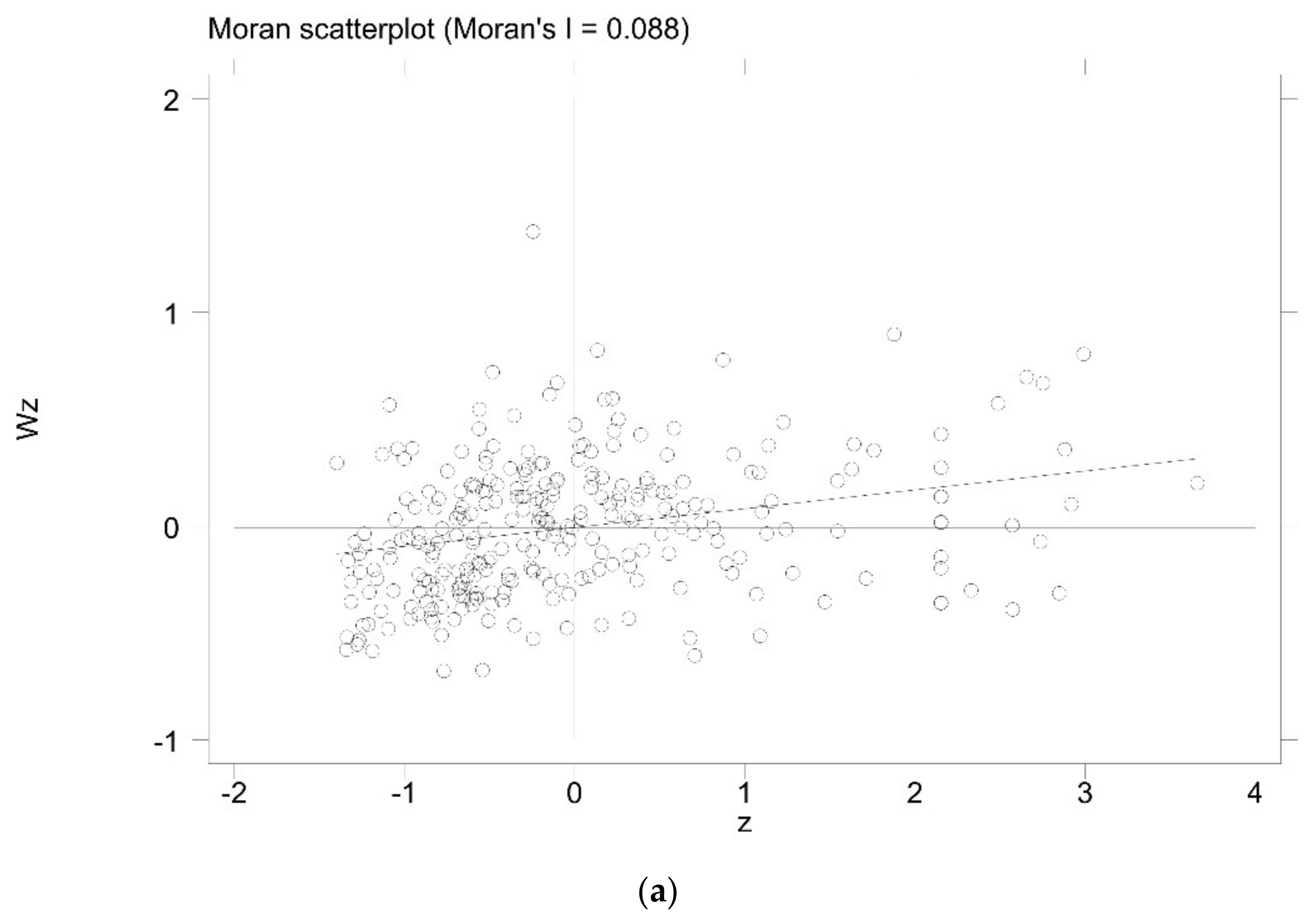
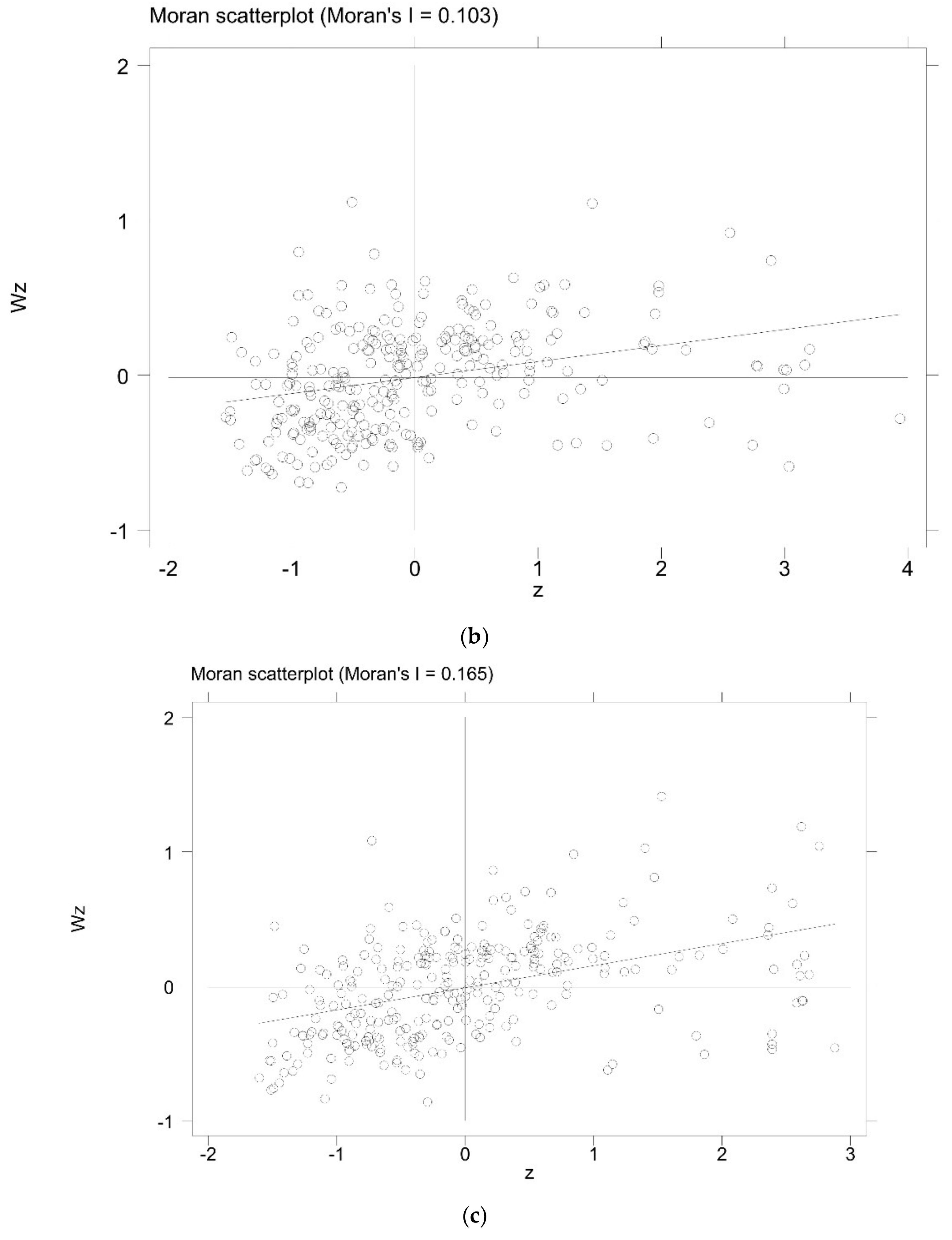
4.2. Spatial Correlation Tests

The spatial correlation test results of city-level CE are shown in Table 2. The global Moran’s I values from 2003 to 2017 are significantly positive at the 1% level and show an overall growth trend, which indicates that the primary assumption of “no spatial autocorrelation” has been significantly rejected, and there is a significant spatial dependency of city-level CE.
The results of Moran scatter plots and LISA cluster maps in the selected years are displayed in Figure 4 and Figure 5, respectively. In Figure 4, the sample cities are mainly located in the first and third quadrants, with most located in the third quadrant. The spatial agglomeration type in the first quadrant is High–High (H-H), which indicates that cities with high CE are surrounded by other cities with high CE, while the cities in the third quadrant are of the Low–Low (L-L) agglomeration type. In Figure 5, cities belonging to L-L clusters are mainly located in the whole territory of Shanxi and Northern Shaanxi, and gradually expanded to Inner Mongolia, Gansu, Ningxia, Hebei, and other regions. With the depletion of coal resources in the eastern region, the layout of China’s coal industry is accelerating to the west, leading to the expansion of low-CE cities to the northwest. H-H clusters are mainly located in the southeast coastal cities and central and eastern Sichuan, and new H-H clusters emerged in Northeast China in 2010, which is closely related to the adjustment of the economic growth model. With the relatively developed economy and high resource utilization, cities in southeast coastal areas have high CE and generate a strong positive radiation effect on the surrounding areas. High–Low (H-L) clusters are scattered over Northeast China, North China, and Northwest China, such as Karamay, Urumqi, Ordos, Beijing, Tianjin, Zhangye, Jiayuguan, Dongying, Dalian, and gradually concentrated in North China during 2003–2017. Zhangye and Jiayuguan have small economy scale. Their environmental pollution is not serious in the process of industrial development. On the contrary, other cities have relatively superior political–economic status in their regions; thus, the CE level can significantly differ from neighboring cities. As the political and economic center of China, although the environmental pollution in the surrounding areas is more serious, strict environmental governance ensures that Beijing is always located in the High–Low CE gathering area.

4.3. Estimation Results

The spatial effect test results based on the residuals of ordinary OLS estimation results show that the statistics of the Spatial Lag Model (SLM) and the Spatial Error Model (SEM) significantly reject the null hypothesis of “no spatial lag” at the 1% level, which indicates the rationality of using a spatial economic model. The results of Wald and LR tests show that the Spatial Dubin Model (SDM) should be adopted. The Hausman test results significantly reject the primary hypothesis of random effect. As a form of technological progress, CE is inevitably affected by the early CE values. Therefore, in this paper, we used the dynamic SDM model (Model D) with double fixed effects in time and space for parameter estimation. The regression results are shown in Table 3. Meanwhile, the estimation results of the ordinary panel model (model A), static SDM model (model B), and non-spatial dynamic panel model (model C) are listed for comparison.
As shown in Table 3, the coefficient symbols of most variables in the four models are consistent. In model B, the coefficient of w.ce is positive at the 1% significance level, indicating that city-level CE has a significant spatial spillover effect. There is a certain strategic competition effect in regional CE, and the CE of surrounding areas can form a positive leading effect on the local area. In model C, the coefficient of l.ce is positive at the 1% significance level, which indicates that CE has the characteristic of path dependence on time. If the CE of the previous period is at a high level, the efficiency level of the next period may continue to rise. The endogeneity and spatial dependency of city-level CE are simultaneously introduced in Model D, which shows better statistical characteristics. Therefore, this paper will focus on the regression results of Model D. The main findings are as follows:
The coefficients of economic development and its square term are significantly negative and positive at the 1% level, respectively; that is to say, there is a significant “U” relationship between economic development and CE. In 2003, 205 of the 283 sample cities exceeded the inflection point of GDP per capita, while in 2017, this was all cities, indicating that economic growth has significantly improved city-level CE in recent years. The higher the economic development, the more obvious the spillover effects of economic agglomeration, energy conservation and emission reduction technology innovation, and environmental governance. Therefore, it is not desirable to improve CE at the expense of city-level economic growth.
The coefficient of industrial structure is negative but not significant, demonstrating that increasing the ratio of secondary industry inhibits the growth of CE to a certain extent, which is consistent with the results of Zeng et al. [37], while the coefficient of industrial structure upgrading is significantly positive. The secondary industry with high energy consumption is still the main driving force of the economic development of most cities in China. With the deepening of supply-side reform, the utilization rate of industrial capacity continues to rise. High-tech manufacturing and equipment manufacturing have brought new comparative advantages to China’s industrial development. In addition, against the background of accelerating the upgrading of industrial structure, the tertiary industry with high added value and low pollution has gradually developed into a new driving force for China’s economic development.
The influence of population density is found to be insignificantly negative on CE. With the development of urbanization, the growth of population density will lead to the expansion of city infrastructure construction scale and energy consumption; thus, increasing CO2 emissions. However, the population agglomeration brings a certain agglomeration effect, which is conducive to the sharing of city infrastructure to improve the technical level, resource utilization, and CE. At present, the agglomeration effect of city population density growth has not fully appeared.
The coefficient of technological progress is significantly negative at the level of 10%. The results prove the rebound effect of China’s city-level technological progress on CE—that is, the potential energy-saving effects caused by technological progress are offset by economic effects, resulting in rapid growth of energy consumption. This is consistent with the research of Huang et al. [102] based on the traditional perspective and the conclusion of Wang et al. [103]. The reason is that the low allocation rate of technological innovation resources, the low conversion rate of scientific and technological achievements, and the significant gap between core key technologies and foreign countries have always restricted China’s technological innovation effect. In addition, the development and application of new technologies often have a time lag.
The coefficient of foreign trade is negative but not significant, which may be attributed to the transformation of China’s trade structure. China’s foreign trade has long been dominated by industrially manufactured products, which accounted for 83% of the total import and export trade in 2017. Against the background of high-quality economic development, the environmental protection requirements of China’s trade products have been continuously improved, and the import and export of high-tech products and low pollution products have been continuously expanded, gradually lowering CO2 emissions. In 2017, the total import and export of high-tech products accounted for 30.6% of the total import and export trade. With the interaction of these two mechanisms, the inhibitory effect of foreign trade on CE is not significant.
The financial development coefficient is significantly negative and passed the 5% significance test, indicating that financial development has significantly inhibited the improvement in city-level CE. In recent years, financial development has stimulated rapid economic expansion, which has also brought a series of environmental problems. The reasons can be summarized as follows. First, the rapid development of finance has stimulated residents’ demands for large commodities such as cars and houses and reduced the financing cost of enterprises. Second, driven by profits, more funds flow into energy-intensive industries with high energy consumption. However, because of the long investment cycle and low rate of return, environmental enterprises cannot obtain strong financial support. Third, excessive intervention from local governments in the financial system has led to the distortion of financial resources.
The coefficient of energy intensity is significantly negative at the 1% level, indicating that the lower the energy intensity, the higher the CE. As a large energy consumption country dominated by fossil energy, coal still occupies a dominant position in China’s energy consumption structure. Uncovering how to realize the clean production and utilization of coal is still a key issue in CO2 emission reduction in the future.
The government intervention coefficient is significantly negative at the level of 1%, indicating that the higher the degree of government intervention, the lower the CE. In order to pursue economic development and political power, city-level governments have shown a productive expenditure bias in the fiscal expenditure structure, investing more funds in the production fields closely related to economic development. Moreover, most orders are undertaken by state-owned enterprises whose investment efficiency is much lower than that of private enterprises [104]. The long-term financial intervention and protectionism from local governments have worsened the local trading environment, resulting in serious resource mismatch and overcapacity, which seriously damage the CE.
The environmental regulation coefficient is positive and significant at 1%, indicating that environmental regulation has a significant improvement effect on city-level CE. Strengthening environmental regulation will help eliminate some backward enterprises with high pollution, and encourage some polluting enterprises to improve their management, technology, and production process to improve resource use efficiency and stimulate the flow of production resources to enterprises with low pollution, low energy consumption, and high efficiency.

4.4. Short- and Long-Term Marginal Effects

Table 4 presents the estimated results of direct effects, indirect effects, and total effects of Model D, which are further decomposed into short- and long-term effects in the time dimension. The direct effect refers to the impact of local factor changes on local CE, and the indirect effect, namely the spatial spillover effect, refers to the impact of local factor changes on the CE of surrounding regions. Overall, the absolute values of long-term effects are greater than short-term effects, indicating the long-term persistence and gradual strengthening characteristics of driving factors on city-level CE. The significance of the short-term effects is relatively high, while the long-term effects are insignificant, implying that the long-term mechanism acting on regional CE has not been formed. In addition, the absolute values of indirect effects are greater than direct effects in the short term, suggesting that the regional spillover effect of driving factors on CE is more significant in the short term.
Firstly, the short-term effects of economic growth and its square term on local CE are significantly negative and positive at the level of 1%, respectively, with the opposite effects on surrounding regions. Local economic growth has produced a significant scale effect, resulting in the increase in local energy consumption and resource agglomeration from surrounding regions. The extensive resource utilization mode inhibits the growth of local CE. With the economic development and the improvement in city environmental governance, high energy-consuming industries have been eliminated or transferred, promoting the progress of environmental efficiency. In the long run, the direct and indirect effects of economic growth on CE are gradually strengthened, and a robust U-shaped curve is formed. The positive externalities produced by economic development have a satisfactory demonstration and driving effect on the surrounding regions, and effectively release the potential of spatial environmental effects. Secondly, the direct effect in the short term of technological progress is insignificant, while the indirect effect is significantly positive at the level of 5%. Because most of China’s technological innovation is dominated by improving economic efficiency, this cannot effectively improve the local CE. Benefiting from the demonstration effect of technological innovation, the CE of surrounding regions shows a spatial positive correlation with the local technological progress. Thirdly, the direct and indirect effects of financial development are significantly negative, which is the result of scale expansion effect brought by financial development. With the acceleration of infrastructure construction, funds flow into high energy-consuming industries, resulting in the rapid growth of energy consumption in the local and surrounding regions. Fourth, the indirect effect of foreign trade is significantly positive. Local governments unilaterally pursue economic effects, resulting in the “pollution shelter” effect, which is unfavorable for local CE. At the same time, the technology spillover effect caused by foreign capital has brought favorable demonstration effects and significant environmental effects to the surrounding areas. However, the technology spillover effect brought by foreign capital has a significant environmental effect on the surrounding regions. Fifth, the direct and indirect effects of energy intensity are significantly negative and positive, respectively. Sixth, the direct and indirect effects of government intervention are significantly negative. The local government expenditure structure dominated by productive expenditure causes a large amount of funds to flow into the production field. At the same time, the excessive intervention of the government distorts the local resource allocation. Under the competition mechanism, in order to achieve the political performance indicators, the surrounding areas have further increased the degree of pre-intervention, resulting in a situation of “one loss for all”. Seventh, the direct and indirect effects of environmental regulation are significantly positive, implying that strengthening environmental regulation is conducive to achieving win–win environmental effects in local and surrounding regions.

5. Conclusions and Policy Recommendations

With the deepening of city economic and social relations, it is important in the pursuit of low-carbon development to investigate city-level CE from a spatial perspective and achieve the win–win goal of economic and social development and environmental benefits. Employing a panel dataset of China’s 283 prefecture-level cities from 2003 to 2017, we used the ESDA methods to explore the temporal and spatial characteristics of city-level CE and constructed the dynamic spatial econometric model to investigate the driving factors. The main conclusions are as follows:
(1)
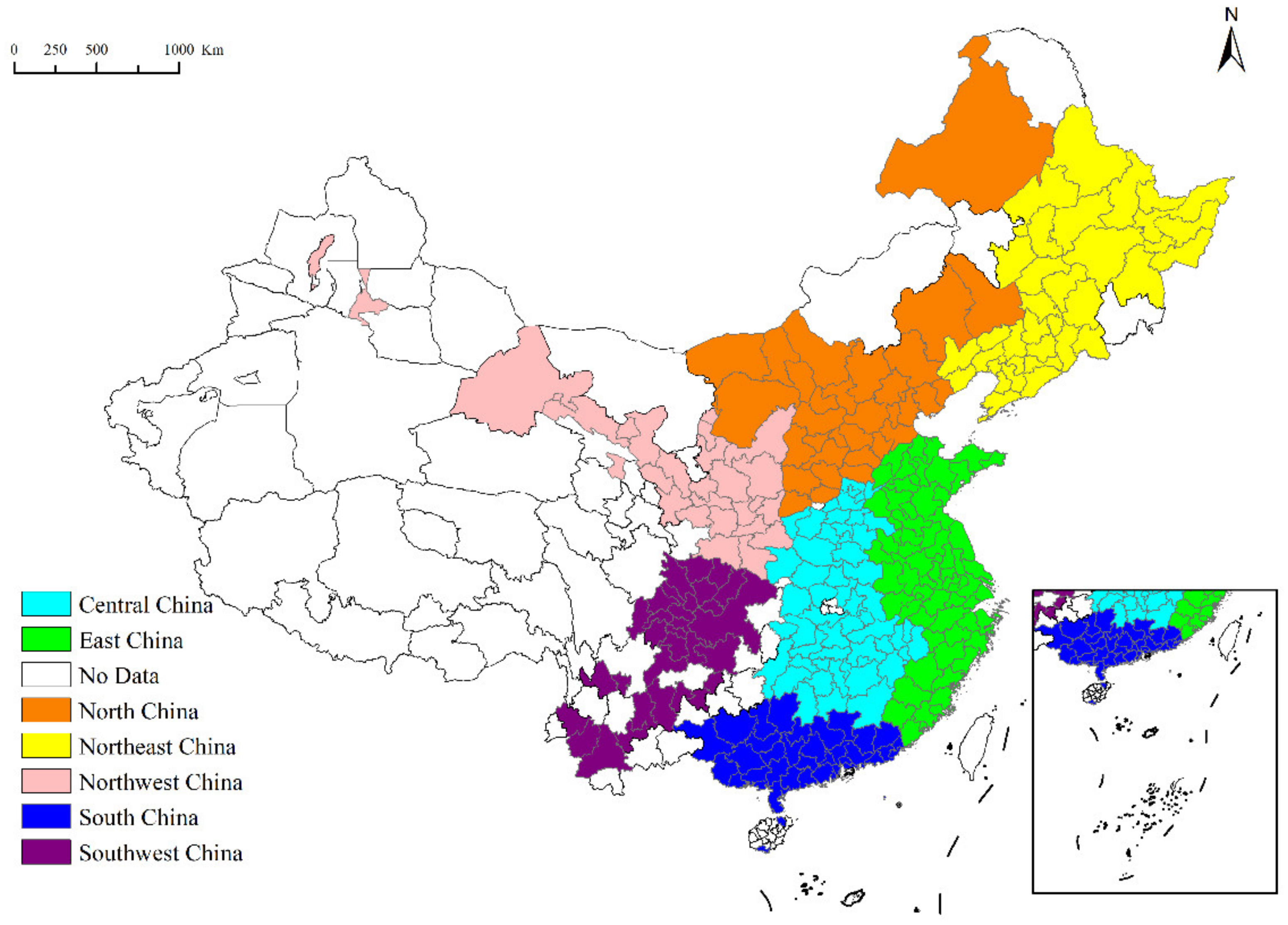
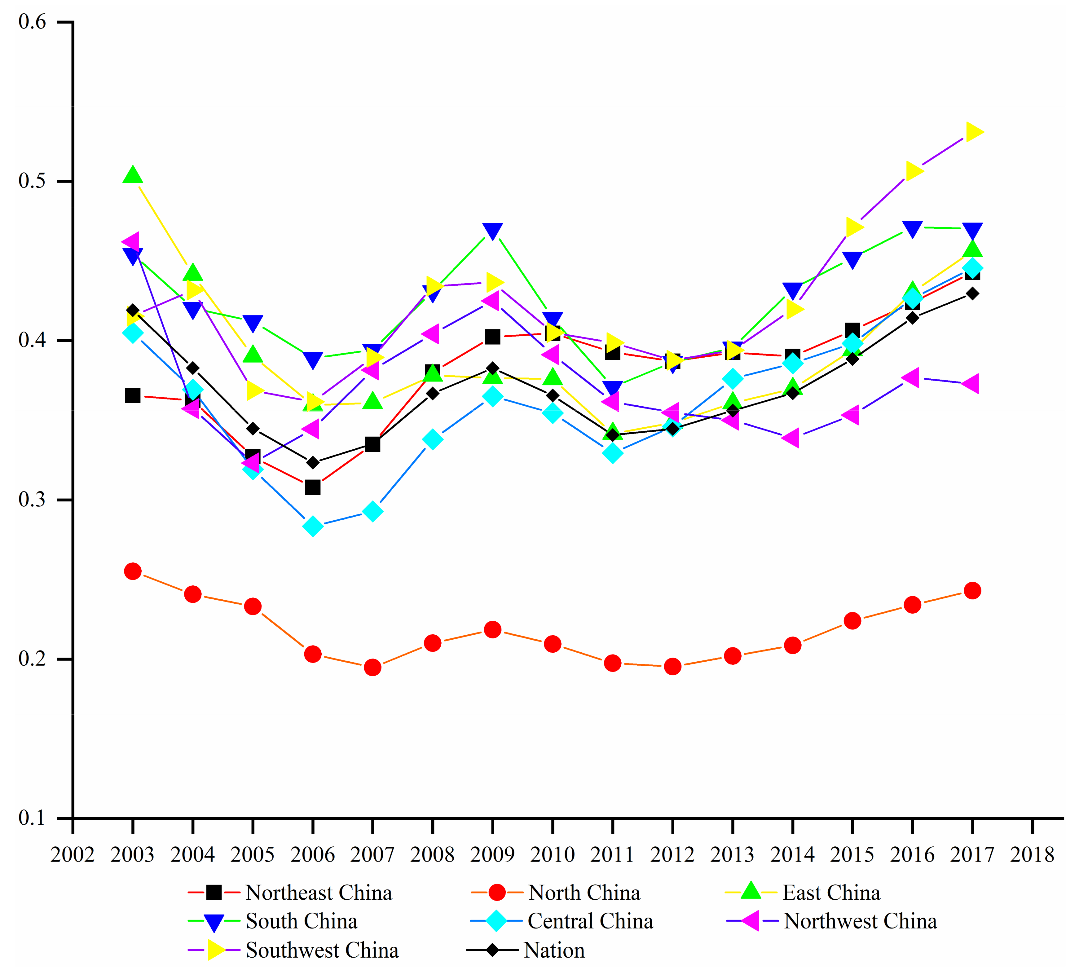
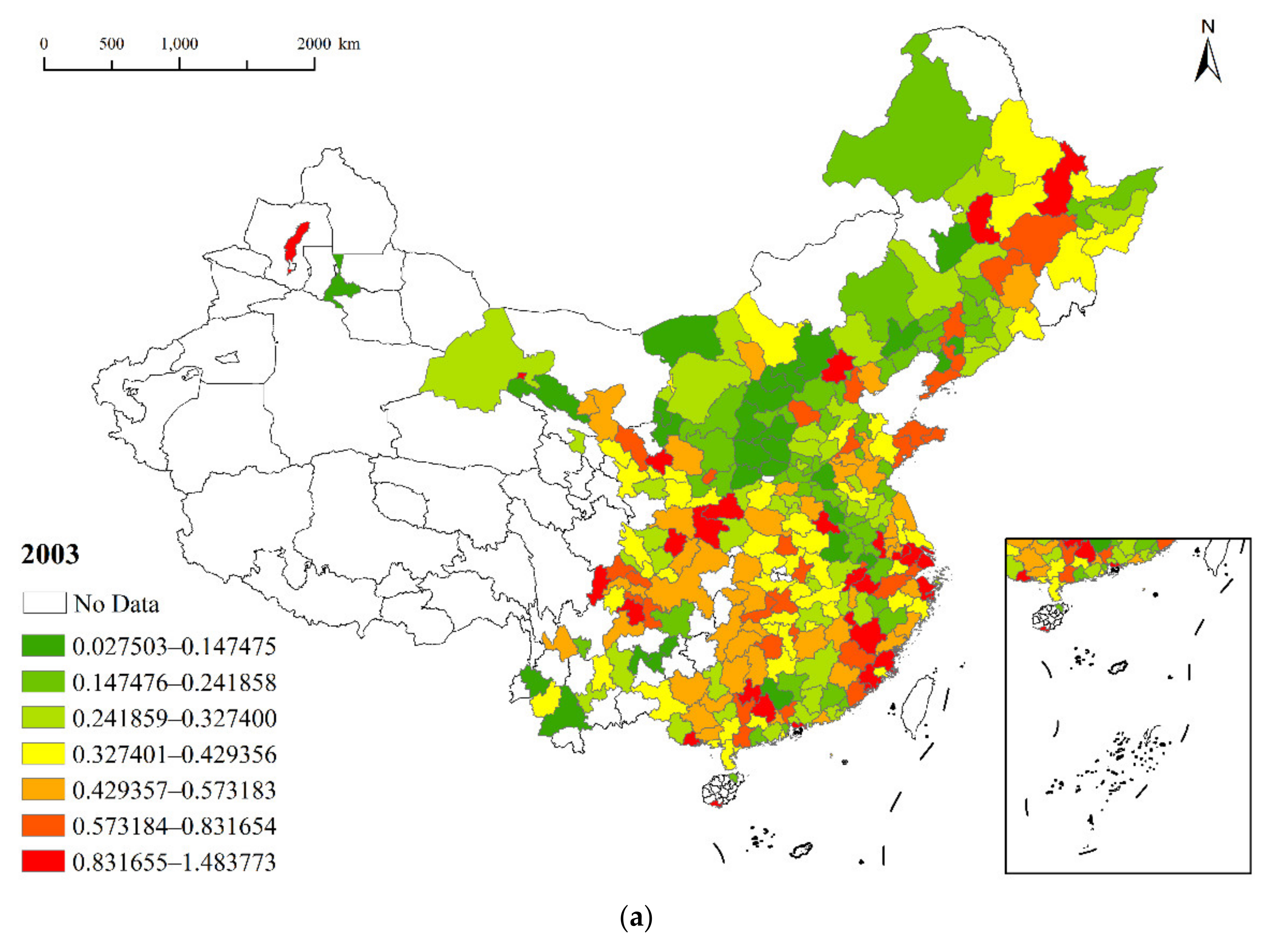
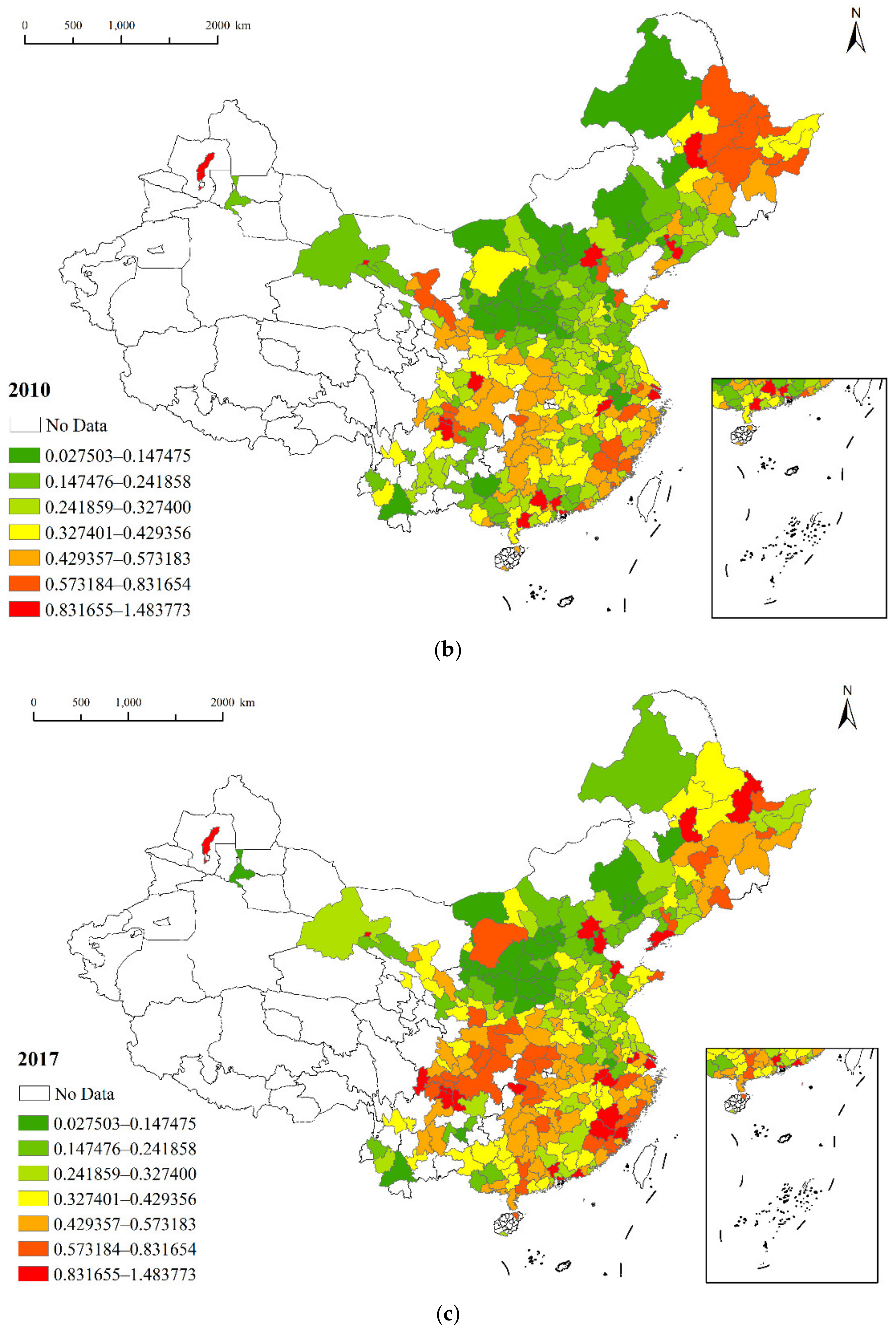
Overall, the average city-level CE from 2003 to 2017 showed a “W”-type growth trend. There were significant spatial heterogeneity characteristics of city-level CE. In 2003, city-level CE was low in the north and high in the south. In 2010, North China, North Central China, and South China formed a continuous low-value area. In 2017, the high-value area of CE expanded significantly.
(2)
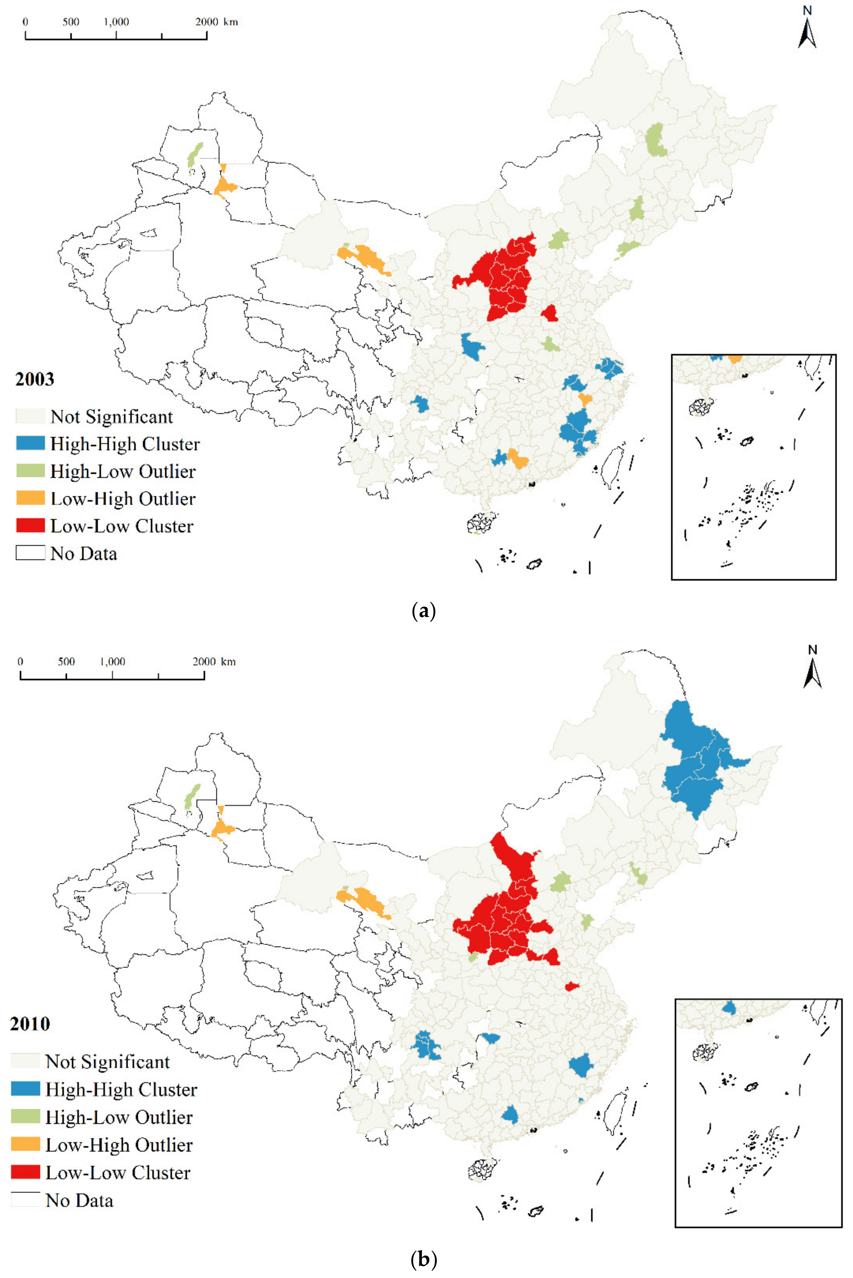
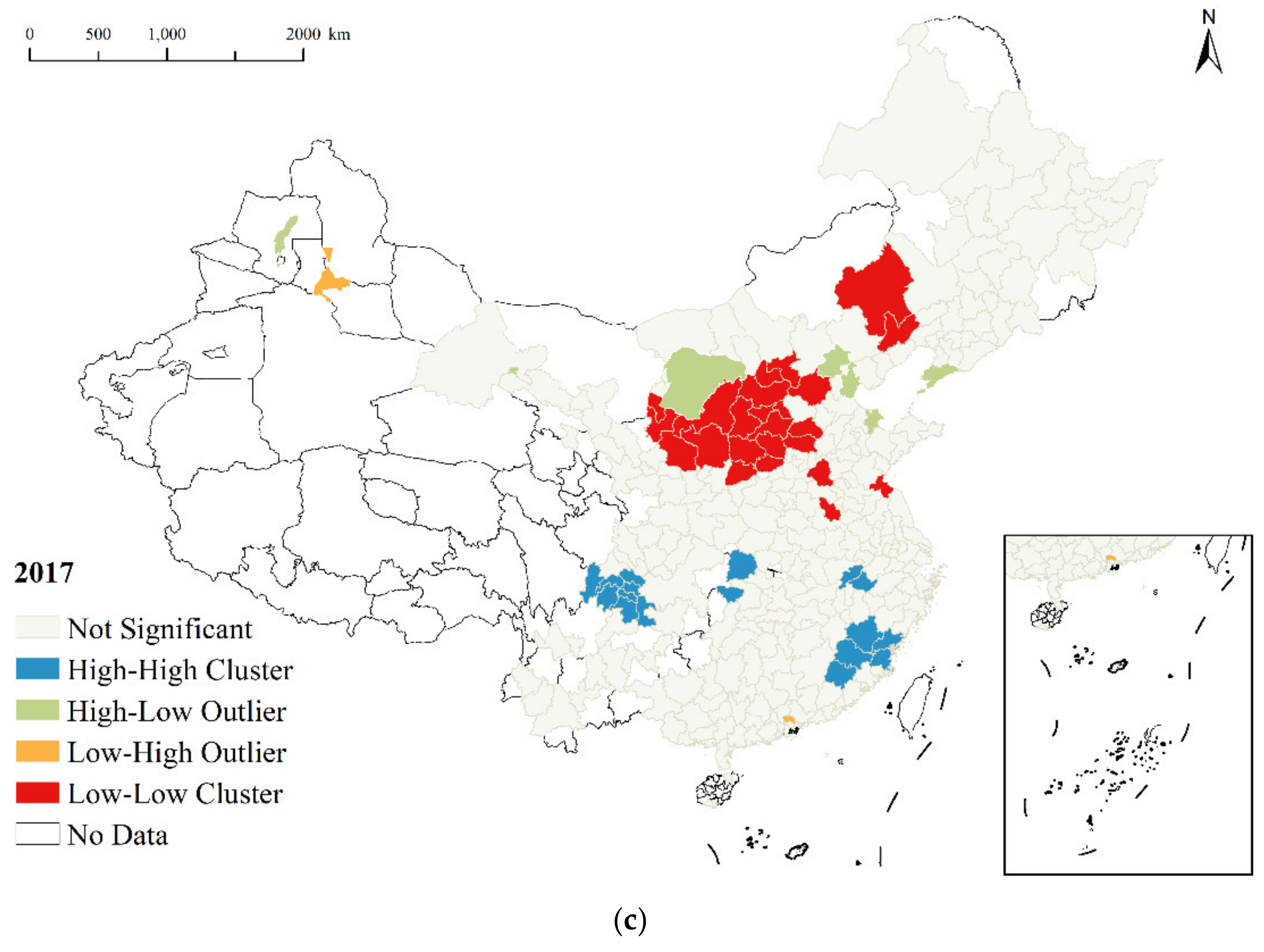
There is a significant spatial dependency of city-level CE. Cities belonging to L-L clusters are mainly located throughout the territory of Shanxi and Northern Shaanxi, and gradually expand to Inner Mongolia, Gansu, Ningxia, Hebei, and other regions. The H-H clusters are mainly located in the southeast coastal cities and central and eastern Sichuan, and new H-H clusters emerged in Northeast China in 2010.
(3)
The empirical results of the dynamic spatial econometric model show that the spatial dependence characteristics of city-level CE co-exist with path dependence on time. There is a significant “U” relationship between economic development and CE. Factors such as industrial structure upgrading and environmental regulation have significant improvement effects on city-level CE, while technological progress, financial development, energy intensity, and government intervention can significantly inhibit city-level CE.
(4)
The long-term effect of driving factors on city-level CE is greater than the short-term effect, and the short-term indirect effect is greater than the direct effect. Factors such as economic development, foreign trade, technological progress, financial development, energy intensity, government intervention, and environmental regulation generate significant spatial spillover effects on city-level CE.
According to the findings above, some policy implications are proposed for improving city-level CE.
Although the average CE values of Chinese cities show an upward trend, there is great potential for improvement. According to the spatial–temporal characteristics of city-level CE, it is necessary to formulate differentiated CE promotion strategies. Cities in South China, East China, and Southwest China should maintain their current CE levels, strengthen technological innovation and city governance, and promote high-quality economic and social development. In addition, their successful policies and measures should be promoted to cities with low CE. Although there has been a short period of high CE in cities in Northeast China, system innovation and industrial structure optimization should still be the key issues of low-carbon development in Northeast China. As the main energy supply areas, cities in North China and Northwest China should focus on improving CE by optimizing industrial and energy structure and improving energy efficiency, for example, by optimizing the development of the modern coal chemical industry, promoting clean and efficient utilization of coal resources, and accelerating the construction of clean energy bases [105].
According to the estimation results of the dynamic spatial econometric model, efforts should be focused on multiple dimensions to improve city-level CE. These dimensions include: facilitating rapid economic growth; promoting the optimization and upgrading of industrial structure, vigorously developing “high-precision and advanced” high-tech industries; supporting the development of strategic emerging industries; advocating a low-carbon lifestyle; strengthening city governance; and improving residents’ awareness of and support for green and low-carbon development. The rebound effect of technological progress on energy consumption cannot be ignored, and it can be alleviated through electricity price reforms [106] and resource taxes [107]. At the same time, optimizing the energy structure and vigorously increasing the proportion of non-fossil energy is also effective [103,108]. Other strategies include deepening low-carbon finance, raising the loan threshold for enterprises with high energy consumption and high emissions, reducing local government intervention in the financial market, and increasing capital market support for low-carbon industries through CO2 emission exchanges, raising the “threshold” of foreign technology introduction and strengthening the spillover effect of advanced technology, strengthening environmental regulation, strengthening the comprehensive effect of industrial policy and market mechanisms in environmental regulation, and enhancing the “precision” regulation effect.
According to the spatial dependency characteristics of city-level CE and the spatial spillover effect of driving factors on city-level CE, it is imperative to establish a regional collaborative emission reduction mechanism and promote the collaborative linkage of energy conservation and emission reduction policies among regions. On the one hand, the joint treatment of pollutants can be carried out through industrial cooperation and resource sharing; on the other hand, when formulating emission reduction policies, we should fully consider neighboring cities, carry out regional docking of relevant energy conservation and emission reduction policies, and strengthen the linkage effect of the implementation of environmental policies among cities. In addition, we should accelerate the construction of low-carbon pilot cities to give full play to their demonstration and leading role. At the same time, the path dependence of carbon efficiency in the time dimension shows that the work of energy conservation and emission reduction is quite urgent and arduous. A long-term mechanism must be established to maintain the continuity and consistency of energy conservation and emission reduction policies over time to continuously promote the regional economy along the path conducive to energy conservation and emission reduction.

Author Contributions

J.T. and X.S. contributed equally to this paper. J.T., investigation; methodology, visualization, writing—original draft; X.S., corresponding author, writing—review and editing, data curation, methodology; J.Z., funding acquisition, supervision, investigation. All authors have read and agreed to the published version of the manuscript.

Funding

This research was funded by Key Think Tank Program on Major Theoretical and Practical Issues of Philosophy and Social Sciences in Shaanxi Province [No. 2021ZD0998], the Natural Science Foundation of China [No. 72004130, 71273206, 52004021, 71810107001, 7169024], the National Key Research and Development Program of China [No.2019YFC1908501], the China Youth Foundation of Humanities and Social Sciences of the Ministry of Education [No.18YJC630148], and Key Projects of Shanghai Soft Science Research Program [No.21692194800].

Informed Consent Statement

Informed consent was obtained from all subjects involved in the study.

Data Availability Statement

Not applicable.

Acknowledgments

We would like to thank the Key Think Tank Program on Major Theoretical and Practical Issues of Philosophy and Social Sciences in Shaanxi Province (No. 2021ZD0998), the Natural Science Foundation of China (No. 72004130, 71273206, 52004021, 71810107001, 7169024), the National Key Research and Development Program of China (No.2019YFC1908501), the China Youth Foundation of Humanities and Social Sciences of the Ministry of Education (No.18YJC630148), and Key Projects of Shanghai Soft Science Research Program (No.21692194800).

Conflicts of Interest

The authors declare that they have no known competing financial interests or personal relationships that could have appeared to influence the work reported in this paper.

References

  1. I.E.A. CO2 Emissions from Fuel Combustion, Highlights. 2012. Available online: https://www.osti.gov/etdeweb/servlets/purl/21589332 (accessed on 1 February 2022).
  2. Lu, Y.; Liu, Y.; Zhou, M. Rebound effect of improved energy efficiency for different energy types: A general equilibrium analysis for China. Energy Econ. 2017, 62, 248–256. [Google Scholar] [CrossRef] [Green Version]
  3. Poluzzi, A.; Guandalini, G.; Romano, M.C. “Potential carbon efficiency” as a new index to track the performance of biofuels production processes. Biomass Bioenergy 2020, 142, 105618. [Google Scholar] [CrossRef]
  4. Wilson, C.; Pettifor, H.; Cassar, E.; Kerr, L.; Wilson, M. The potential contribution of disruptive low-carbon innovations to 1.5 °C climate mitigation. Energy Effic. 2019, 12, 423–440. [Google Scholar] [CrossRef] [Green Version]
  5. I.E.A. World Energy Outlook 2007: China and India Insights. 2007. Available online: https://www.iea.org/reports/world-energy-outlook-2007 (accessed on 1 February 2022).
  6. Gouldson, A.; Colenbrander, S.; Sudmant, A.; Papargyropoulou, E.; Kerr, N.; McAnulla, F.; Hall, S. Cities and climate change mitigation: Economic opportunities and governance challenges in Asia. Cities 2016, 54, 11–19. [Google Scholar] [CrossRef] [Green Version]
  7. Rosenzweig, C.; Solecki, W.; Hammer, S.A.; Mehrotra, S. Cities lead the way in climate-change action. Nature 2010, 467, 909–911. [Google Scholar] [CrossRef]
  8. Zhang, Y. Interregional Supply-driven Carbon Emission Spillover-feedback Effects. J. China Populat. Resourc. Environ. 2016, 26, 55–62. [Google Scholar]
  9. Sun, L.; Wang, Q.; Zhou, P.; Cheng, F. Effects of carbon emission transfer on economic spillover and carbon emission reduction in China. J. Clean. Prod. 2016, 112, 1432–1442. [Google Scholar] [CrossRef]
  10. Kaya, Y.; Yokobori, K. Environment, Energy, and Economy: Strategies for Sustainability; United Nations University Press: Tokyo, Japan, 1997. [Google Scholar]
  11. Mielnik, O.; Goldemberg, J. The evolution of the “carbonization index” in developing countries. Energy Policy 1999, 27, 307–308. [Google Scholar] [CrossRef]
  12. Sun, J.W. The decrease of CO2 emission intensity is decarbonization at national and global levels. Energy Policy 2005, 33, 975–978. [Google Scholar] [CrossRef]
  13. Ramanathan, R. Combining indicators of energy consumption and CO2 emissions: A cross-country comparison. Int. J. Glob. Energy Issues 2002, 17, 214–227. [Google Scholar] [CrossRef]
  14. Ramanathan, R. A multi-factor efficiency perspective to the relationships among world GDP, energy consumption and carbon dioxide emissions. Technol. Forecast. Soc. Change 2006, 73, 483–494. [Google Scholar] [CrossRef]
  15. Molinos-Senante, M.; Sala-Garrido, R.; Hernandez-Sancho, F. Development and application of the Hicks-Moorsteen productivity index for the total factor productivity assessment of wastewater treatment plants. J. Clean. Prod. 2016, 112, 3116–3123. [Google Scholar] [CrossRef]
  16. Song, M.; An, Q.; Zhang, W.; Wang, Z.; Wu, J. Environmental efficiency evaluation based on data envelopment analysis: A review. Renew. Sustain. Energy Rev. 2012, 16, 4465–4469. [Google Scholar] [CrossRef]
  17. Meng, F.; Su, B.; Thomson, E.; Zhou, D.; Zhou, P. Measuring China’s regional energy and carbon emission efficiency with DEA models: A survey. Appl. Energy 2016, 183, 1–21. [Google Scholar] [CrossRef]
  18. Shang, Y.; Liu, H.; Lv, Y. Total factor energy efficiency in regions of China: An empirical analysis on SBM-DEA model with undesired generation. J. King Saud Univ.-Sci. 2020, 32, 1925–1931. [Google Scholar] [CrossRef]
  19. Cecchini, L.; Venanzi, S.; Pierri, A.; Chiorri, M. Environmental efficiency analysis and estimation of CO2 abatement costs in dairy cattle farms in Umbria (Italy): A SBM-DEA model with undesirable output. J. Clean. Prod. 2018, 197, 895–907. [Google Scholar] [CrossRef]
  20. Iftikhar, Y.; Wang, Z.; Zhang, B.; Wang, B. Energy and CO2 emissions efficiency of major economies: A network DEA approach. Energy 2018, 147, 197–207. [Google Scholar] [CrossRef]
  21. Färe, R.; Grosskopf, S.; Lovell, C.A.K.; Pasurka, C. Multilateral productivity comparisons when some outputs are undesirable: A nonparametric approach. Rev. Econ. Stat. 1989, 71, 90–98. [Google Scholar] [CrossRef]
  22. Färe, R.; Grosskopf, S.; Pasurka, C.A. Environmental production functions and environmental directional distance functions. Energy 2007, 32, 1055–1066. [Google Scholar] [CrossRef]
  23. Färe, R.; Grosskopf, S. Directional distance functions and slacks-based measures of efficiency. Eur. J. Oper. Res. 2010, 200, 320–322. [Google Scholar] [CrossRef]
  24. Liu, Y.; Zhao, G.; Zhao, Y. An analysis of Chinese provincial carbon dioxide emission efficiencies based on energy consumption structure. Energy Policy 2016, 96, 524–533. [Google Scholar] [CrossRef]
  25. Wang, G.; Deng, X.; Wang, J.; Zhang, F.; Liang, S. Carbon emission efficiency in China: A spatial panel data analysis. China Econ. Rev. 2019, 56, 101313. [Google Scholar] [CrossRef]
  26. Li, J.; Cheng, Z. Study on total-factor carbon emission efficiency of China’s manufacturing industry when considering technology heterogeneity. J. Clean. Prod. 2020, 260, 121021. [Google Scholar] [CrossRef]
  27. Yan, D.; Lei, Y.; Li, L.; Song, W. Carbon emission efficiency and spatial clustering analyses in China’s thermal power industry: Evidence from the provincial level. J. Clean. Prod. 2017, 156, 518–527. [Google Scholar] [CrossRef]
  28. Zhu, R.; Zhao, R.; Sun, J.; Xiao, L.; Jiao, S.; Chuai, X.; Zhang, L.; Yang, Q. Temporospatial pattern of carbon emission efficiency of China’s energy-intensive industries and its policy implications. J. Clean. Prod. 2021, 286, 125507. [Google Scholar] [CrossRef]
  29. Cheng, Z.; Li, L.; Liu, J.; Zhang, H. Total-factor carbon emission efficiency of China’s provincial industrial sector and its dynamic evolution. Renew. Sustain. Energy Rev. 2018, 94, 330–339. [Google Scholar] [CrossRef]
  30. Yao, X.; Zhou, H.; Zhang, A.; Li, A. Regional energy efficiency, carbon emission performance and technology gaps in China: A meta-frontier non-radial directional distance function analysis. Energy Policy 2015, 84, 142–154. [Google Scholar] [CrossRef]
  31. Yao, X.; Guo, C.; Shao, S.; Jiang, Z. Total-factor CO2 emission performance of China’s provincial industrial sector: A meta-frontier non-radial Malmquist index approach. Appl. Energy 2016, 184, 1142–1153. [Google Scholar] [CrossRef]
  32. Zhang, W.; Tang, X.; Yang, G.; Zha, D. Decomposition of CO2 emission intensity in Chinese MIs through a development mode extended LMDI method combined with a production-theoretical approach. Sci. Total Environ. 2020, 702, 134787. [Google Scholar] [CrossRef]
  33. Fan, M.; Shao, S.; Yang, L. Combining global Malmquist-Luenberger index and generalized method of moments to investigate industrial total factor CO2 emission performance: A case of Shanghai (China). Energy Policy 2015, 79, 189–201. [Google Scholar] [CrossRef]
  34. Du, K.; Li, J. Towards a green world: How do green technology innovations affect total-factor carbon productivity. Energy Policy 2019, 131, 240–250. [Google Scholar] [CrossRef]
  35. Tan, X.; Choi, Y.; Wang, B.; Huang, X. Does China’s carbon regulatory policy improve total factor carbon efficiency? A fixed-effect panel stochastic frontier analysis. Technol. Forecast. Soc. Change 2020, 160, 120222. [Google Scholar] [CrossRef]
  36. Zhou, Y.; Liu, W.; Lv, X.; Chen, X.; Shen, M. Investigating interior driving factors and cross-industrial linkages of carbon emission efficiency in China’s construction industry: Based on Super-SBM DEA and GVAR model. J. Clean. Prod. 2019, 241, 118322. [Google Scholar] [CrossRef]
  37. Zeng, L.; Lu, H.; Liu, Y.; Zhou, Y.; Hu, H. Analysis of regional differences and influencing factors on China’s carbon emission efficiency in 2005–2015. Energies 2019, 12, 3081. [Google Scholar] [CrossRef] [Green Version]
  38. Marbuah, G.; Amuakwa-Mensah, F. Spatial analysis of emissions in Sweden. Energy Econ. 2017, 68, 383–394. [Google Scholar] [CrossRef] [Green Version]
  39. Zhou, H.; Jiang, M.; Huang, Y.; Wang, Q. Directional spatial spillover effects and driving factors of haze pollution in North China Plain. Resour. Conserv. Recycl. 2021, 169, 105475. [Google Scholar] [CrossRef]
  40. Ning, Y.; Miao, L.; Ding, T.; Zhang, B. Carbon emission spillover and feedback effects in China based on a multiregional input-output model. Resour. Conserv. Recycl. 2019, 141, 211–218. [Google Scholar] [CrossRef]
  41. Chu, X.; Geng, H.; Guo, W. How does energy misallocation affect carbon emission efficiency in China? An empirical study based on the spatial econometric model. Sustainability 2019, 11, 2115. [Google Scholar] [CrossRef] [Green Version]
  42. Zhang, L.; Xiong, L.; Cheng, B.; Yu, C. How does foreign trade influence China’s carbon productivity? Based on panel spatial lag model analysis. Struct. Change Econ. Dyn. 2018, 47, 171–179. [Google Scholar] [CrossRef]
  43. Xie, Z.; Wu, R.; Wang, S. How technological progress affects the carbon emission efficiency? Evidence from national panel quantile regression. J. Clean. Prod. 2021, 307, 127133. [Google Scholar] [CrossRef]
  44. Sun, W.; Huang, C. How does urbanization affect carbon emission efficiency? Evidence from China. J. Clean. Prod. 2020, 272, 122828. [Google Scholar] [CrossRef]
  45. Wang, K.; Wu, M.; Sun, Y.; Shi, X.; Sun, A.; Zhang, P. Resource abundance, industrial structure, and regional carbon emissions efficiency in China. Resour. Policy 2019, 60, 203–214. [Google Scholar] [CrossRef]
  46. Andersen, P.; Petersen, N.C. A Procedure for Ranking Efficient Units in Data Envelopment Analysis. Manag. Sci. 1993, 39, 1261–1264. [Google Scholar] [CrossRef]
  47. Tone, K. A slacks-based measure of super-efficiency in data envelopment analysis. Eur. J. Oper. Res. 2002, 143, 32–41. [Google Scholar] [CrossRef] [Green Version]
  48. Zhao, P.; Zeng, L.; Lu, H.; Zhou, Y.; Hu, H.; Wei, X.-Y. Green economic efficiency and its influencing factors in China from 2008 to 2017: Based on the super-SBM model with undesirable outputs and spatial Dubin model. Sci. Total Environ. 2020, 741, 140026. [Google Scholar] [CrossRef]
  49. Zhang, J.; Zeng, W.; Wang, J.; Yang, F.; Jiang, H. Regional low-carbon economy efficiency in China: Analysis based on the Super-SBM model with CO2 emissions. J. Clean. Prod. 2017, 163, 202–211. [Google Scholar] [CrossRef]
  50. Zhang, Y.; Chen, X.; Mao, Y.; Shuai, C.; Jiao, L.; Wu, Y. Analysis of resource allocation and PM2.5 pollution control efficiency: Evidence from 112 Chinese cities. Ecol. Indic. 2021, 127, 107705. [Google Scholar] [CrossRef]
  51. Bian, J.; Zhang, Y.; Shuai, C.; Shen, L.; Ren, H.; Wang, Y. Have cities effectively improved ecological well-being performance? Empirical analysis of 278 Chinese cities. J. Clean. Prod. 2020, 245, 118913. [Google Scholar] [CrossRef]
  52. Acheampong, A.O. Economic growth, CO2 emissions and energy consumption: What causes what and where? Energy Econ. 2018, 74, 677–692. [Google Scholar] [CrossRef]
  53. Abid, M. Does economic, financial and institutional developments matter for environmental quality? A comparative analysis of EU and MEA countries. J. Environ. Manag. 2017, 188, 183–194. [Google Scholar] [CrossRef]
  54. Chen, Y.; Guo, F.; Wang, J.; Cai, W.; Wang, C.; Wang, K. Provincial and gridded population projection for China under shared socioeconomic pathways from 2010 to 2100. Sci. Data 2020, 7, 83. [Google Scholar] [CrossRef] [Green Version]
  55. Zhou, P.; Ang, B.W.; Wang, H. Energy and CO2 emission performance in electricity generation: A non-radial directional distance function approach. Eur. J. Oper. Res. 2012, 221, 625–635. [Google Scholar] [CrossRef]
  56. Elhorst, J.P. Spatial Econometrics: From Cross Sectional Data to Spatial Panels; Springer: Berlin/Heidelberg, Germany, 2014; ISBN 978-1-4200-7287-7. [Google Scholar]
  57. Shao, S.; Yang, L.; Yu, M.; Yu, M. Estimation, characteristics, and determinants of energy-related industrial CO2 emissions in Shanghai (China), 1994–2009. Energy Policy 2011, 39, 6476–6494. [Google Scholar] [CrossRef]
  58. Changqing, L.; Lei, L.; Ping, W. Measurement of capital stock of cities at prefecture level and above in China. Urban Probl. 2017, 0, 67–72. [Google Scholar]
  59. Su, Y.; Chen, X.; Li, Y.; Liao, J.; Ye, Y.; Zhang, H.; Huang, N.; Kuang, Y. China’s 19-year city-level carbon emissions of energy consumptions, driving forces and regionalized mitigation guidelines. Renew. Sustain. Energy Rev. 2014, 35, 231–243. [Google Scholar] [CrossRef]
  60. Wang, Y.; Li, G. Mapping urban CO2 emissions using DMSP/OLS ‘city lights’ satellite data in China. Environ. Plan. A 2017, 49, 248–251. [Google Scholar] [CrossRef] [Green Version]
  61. Sheng, P.; Li, J.; Zhai, M.; Huang, S. Coupling of economic growth and reduction in carbon emissions at the efficiency level: Evidence from China. Energy 2020, 213, 118747. [Google Scholar] [CrossRef]
  62. Antweiler, W.; Copeland, B.R.; Taylor, M.S. Is free trade good for the environment? Am. Econ. Rev. 2001, 91, 877–908. [Google Scholar] [CrossRef] [Green Version]
  63. Almodóvar, P.; Saiz-Briones, J.; Silverman, B.S. Learning through foreign market participation: The relative benefits of exporting, importing, and foreign direct investment. J. Technol. Transf. 2014, 39, 915–944. [Google Scholar] [CrossRef]
  64. Zhao, H.; Lin, B. Impact of foreign trade on energy efficiency in China’s textile industry. J. Clean. Prod. 2020, 245, 118878. [Google Scholar] [CrossRef]
  65. Danish; Ud-Din Khan, S.; Ahmad, A. Testing the pollution haven hypothesis on the pathway of sustainable development: Accounting the role of nuclear energy consumption. Nucl. Eng. Technol. 2021, 53, 2746–2752. [Google Scholar] [CrossRef]
  66. Lin, B.; Xu, M. Does China become the “pollution heaven” in South-South trade? Evidence from Sino-Russian trade. Sci. Total Environ. 2019, 666, 964–974. [Google Scholar] [CrossRef] [PubMed]
  67. Duan, Y.; Jiang, X. Pollution haven or pollution halo? A Re-evaluation on the role of multinational enterprises in global CO2 emissions. Energy Econ. 2021, 97, 105181. [Google Scholar] [CrossRef]
  68. Duan, Y.; Yan, B. Economic gains and environmental losses from international trade: A decomposition of pollution intensity in China’s value-added trade. Energy Econ. 2019, 83, 540–554. [Google Scholar] [CrossRef]
  69. Ren, S.; Li, X.; Yuan, B.; Li, D.; Chen, X. The effects of three types of environmental regulation on eco-efficiency: A cross-region analysis in China. J. Clean. Prod. 2018, 173, 245–255. [Google Scholar] [CrossRef]
  70. Sinn, H.-W. Public policies against global warming: A supply side approach. Int. Tax Public Financ. 2008, 15, 360–394. [Google Scholar] [CrossRef]
  71. Van Der Werf, E.; Di Maria, C. Imperfect environmental policy and polluting emissions: The green paradox and beyond. Int. Rev. Environ. Resour. Econ. 2012, 6, 153–194. [Google Scholar] [CrossRef] [Green Version]
  72. Smulders, S.; Tsur, Y.; Zemel, A. Announcing climate policy: Can a green paradox arise without scarcity? J. Environ. Econ. Manag. 2012, 64, 364–376. [Google Scholar] [CrossRef] [Green Version]
  73. Lanoie, P.; Laurent-Lucchetti, J.; Johnstone, N.; Ambec, S. Environmental policy, innovation and performance: New insights on the porter hypothesis. J. Econ. Manag. Strateg. 2011, 20, 803–842. [Google Scholar] [CrossRef] [Green Version]
  74. Floros, N.; Vlachou, A. Energy demand and energy-related CO2 emissions in Greek manufacturing: Assessing the impact of a carbon tax. Energy Econ. 2005, 27, 387–413. [Google Scholar] [CrossRef]
  75. Zhang, Y.; Song, Y. Environmental regulations, energy and environment efficiency of China’s metal industries: A provincial panel data analysis. J. Clean. Prod. 2021, 280, 124437. [Google Scholar] [CrossRef]
  76. Pei, Y.; Zhu, Y.; Liu, S.; Wang, X.; Cao, J. Environmental regulation and carbon emission: The mediation effect of technical efficiency. J. Clean. Prod. 2019, 236, 117599. [Google Scholar] [CrossRef]
  77. Yasmeen, H.; Tan, Q.; Zameer, H.; Tan, J.; Nawaz, K. Exploring the impact of technological innovation, environmental regulations and urbanization on ecological efficiency of China in the context of COP21. J. Environ. Manag. 2020, 274, 111210. [Google Scholar] [CrossRef]
  78. Hu, W.; Wang, D. How does environmental regulation influence China’s carbon productivity? An empirical analysis based on the spatial spillover effect. J. Clean. Prod. 2020, 257, 120484. [Google Scholar] [CrossRef]
  79. Zhou, Y.; Kong, Y.; Sha, J.; Wang, H. The role of industrial structure upgrades in eco-efficiency evolution: Spatial correlation and spillover effects. Sci. Total Environ. 2019, 687, 1327–1336. [Google Scholar] [CrossRef]
  80. Han, Y.; Zhang, F.; Huang, L.; Peng, K.; Wang, X. Does industrial upgrading promote eco-efficiency?—A panel space estimation based on Chinese evidence. Energy Policy 2021, 154, 112286. [Google Scholar] [CrossRef]
  81. Zhou, X.-Y.; Lei, K.; Meng, W.; Khu, S.-T. Industrial structural upgrading and spatial optimization based on water environment carrying capacity. J. Clean. Prod. 2017, 165, 1462–1472. [Google Scholar] [CrossRef]
  82. Wu, J. The Choice of China’s Growth Model; Shanghai Far East Publishers: Shanghai, China, 2013. [Google Scholar]
  83. Borck, R.; Schrauth, P. Population density and urban air quality. Reg. Sci. Urban Econ. 2021, 86, 103596. [Google Scholar] [CrossRef]
  84. Clark, T.A. Metropolitan density, energy efficiency and carbon emissions: Multi-attribute tradeoffs and their policy implications. Energy Policy 2013, 53, 413–428. [Google Scholar] [CrossRef]
  85. Liu, S.; Xia, X.H.; Tao, F.; Chen, X.Y. Assessing urban carbon emission efficiency in China: Based on the global data envelopment analysis. Energy Procedia 2018, 152, 762–767. [Google Scholar] [CrossRef]
  86. Wang, Q.; Wang, S. Why does China’s carbon intensity decline and India’s carbon intensity rise? A decomposition analysis on the sectors. J. Clean. Prod. 2020, 265, 121569. [Google Scholar] [CrossRef]
  87. Liu, N.; Ma, Z.; Kang, J. Changes in carbon intensity in China’s industrial sector: Decomposition and attribution analysis. Energy Policy 2015, 87, 28–38. [Google Scholar] [CrossRef]
  88. Su, B.; Ang, B.W. Demand contributors and driving factors of Singapore’s aggregate carbon intensities. Energy Policy 2020, 146, 111817. [Google Scholar] [CrossRef]
  89. Song, M.; Wu, J.; Song, M.; Zhang, L.; Zhu, Y. Spatiotemporal regularity and spillover effects of carbon emission intensity in China’s Bohai Economic Rim. Sci. Total Environ. 2020, 740, 140184. [Google Scholar] [CrossRef]
  90. Zhang, F.; Deng, X.; Phillips, F.; Fang, C.; Wang, C. Impacts of industrial structure and technical progress on carbon emission intensity: Evidence from 281 cities in China. Technol. Forecast. Soc. Change 2020, 154, 119949. [Google Scholar] [CrossRef]
  91. Cheng, Z.; Li, L.; Liu, J. Industrial structure, technical progress and carbon intensity in China’s provinces. Renew. Sustain. Energy Rev. 2018, 81, 2935–2946. [Google Scholar] [CrossRef]
  92. Dong, F.; Yu, B.; Hadachin, T.; Dai, Y.; Wang, Y.; Zhang, S.; Long, R. Drivers of carbon emission intensity change in China. Resour. Conserv. Recycl. 2018, 129, 187–201. [Google Scholar] [CrossRef]
  93. Tamazian, A.; Rao, B.B. Do economic, financial and institutional developments matter for environmental degradation? Evidence from transitional economies. Energy Econ. 2010, 32, 137–145. [Google Scholar] [CrossRef] [Green Version]
  94. Zagorchev, A.; Vasconcellos, G.; Bae, Y. Financial development, technology, growth and performance: Evidence from the accession to the EU. J. Int. Financ. Mark. Inst. Money 2011, 21, 743–759. [Google Scholar] [CrossRef]
  95. Acheampong, A.O.; Amponsah, M.; Boateng, E. Does financial development mitigate carbon emissions? Evidence from heterogeneous financial economies. Energy Econ. 2020, 88, 104768. [Google Scholar] [CrossRef]
  96. Sadorsky, P. Financial development and energy consumption in Central and Eastern European frontier economies. Energy Policy 2011, 39, 999–1006. [Google Scholar] [CrossRef]
  97. Yan, B.; Wu, L.; Wang, X.H.; Wu, J. How can environmental intervention work during rapid urbanization? Examining the moderating effect of environmental performance-based accountability in China. Environ. Impact Assess. Rev. 2021, 86, 106476. [Google Scholar] [CrossRef]
  98. Cheng, S.; Fan, W.; Chen, J.; Meng, F.; Liu, G.; Song, M.; Yang, Z. The impact of fiscal decentralization on CO2 emissions in China. Energy 2020, 192, 116685. [Google Scholar] [CrossRef]
  99. Krajewski, P.; Mackiewicz, M. The role of capital and labour in shaping the environmental effects of fiscal stimulus. J. Clean. Prod. 2019, 216, 323–332. [Google Scholar] [CrossRef]
  100. Fan, W.; Li, L.; Wang, F.; Li, D. Driving factors of CO2 emission inequality in China: The role of government expenditure. China Econ. Rev. 2020, 64, 101545. [Google Scholar] [CrossRef]
  101. Zhang, K.-Y.; Wang, Y.-Z.; Peng, Z.Y.S. The Evolution, Causes and Influencing Factors of South-North Differentiation within the Western China Zhang. Economist 2021, 3, 51–62. [Google Scholar] [CrossRef]
  102. Huang, J.; Chen, X.; Yu, K.; Cai, X. Effect of technological progress on carbon emissions: New evidence from a decomposition and spatiotemporal perspective in China. J. Environ. Manag. 2020, 274, 110953. [Google Scholar] [CrossRef]
  103. Wang, S.; Zeng, J.; Liu, X. Examining the multiple impacts of technological progress on CO2 emissions in China: A panel quantile regression approach. Renew. Sustain. Energy Rev. 2019, 103, 140–150. [Google Scholar] [CrossRef]
  104. Chen, S.; Sun, Z.; Tang, S.; Wu, D. Government intervention and investment efficiency: Evidence from China. J. Corp. Financ. 2011, 17, 259–271. [Google Scholar] [CrossRef]
  105. National Energy Administration. The 13th Five-Year Plan for Coal Industry Development. Available online: http://www.gov.cn/zhengce/content/2017-02/03/content_5164865.htm (accessed on 12 January 2017).
  106. Lin, B.; Tian, P. The energy rebound effect in China’s light industry: A translog cost function approach. J. Clean. Prod. 2016, 112, 2793–2801. [Google Scholar] [CrossRef]
  107. Binswanger, M. Technological progress and sustainable development: What about the rebound effect? Ecol. Econ. 2001, 36, 119–132. [Google Scholar] [CrossRef]
  108. Chen, J.; Gao, M.; Shahbaz, M.; Cheng, S.; Song, M. An improved decomposition approach toward energy rebound effects in China: Review since 1992. Renew. Sustain. Energy Rev. 2021, 145, 111141. [Google Scholar] [CrossRef]
Figure 1. Study area.
Energies 15 02536 g001
Figure 2. Temporal variations in average city-level CE from 2003 to 2017.
Energies 15 02536 g002
Figure 3. Spatial distributions of city-level CE (a) 2003, (b) 2010, (c) 2017.
Energies 15 02536 g003aEnergies 15 02536 g003b
Figure 4. Moran scatter plots of citylevel CE (a) 2003, (b) 2010, (c) 2017.
Energies 15 02536 g004aEnergies 15 02536 g004b
Figure 5. LISA map of city-level CE in (a) 2003, (b) 2010, and (c) 2017.
Energies 15 02536 g005aEnergies 15 02536 g005b
Table 1. Descriptive statistics of variables, 2003–2017.
VariableMeanStd. Dev.MinMax
GDP1275.8561912.39631.44623,402.05
Capital2544.2544025.46517.3252,548.78
Labor260.1852612.2879.1738,230
Energy1292.3991299.46726.24811,858.96
CO2 emission34.197435.5830.546265.208
Carbon efficiency0.3710.2250.0281.484
Economic development9.910.8527.24412.698
Industrial structure0.4840.1110.090.91
Industrial structure upgrading0.8680.5110.09410.766
Population density5.7290.9081.5477.886
Technological progress6.1631.8450.69311.578
Financial development2.3151.5040.14231.586
Foreign trade0.2530.4760.000027.018
Energy intensity1.5151.2110.12114.842
Government intervention0.2080.1520.0312.422
Environmental regulation0.6590.1580.16390.978
Table 2. Global Moran’s I of city-level CE from 2003 to 2017.
Year20032004200520062007200820092010
I0.0880.0850.1080.10.1040.1190.1250.103
Z(I)4.9124.7446.0085.5935.8036.586.8885.739
p-value0.0000.0000.0000.0000.0000.0000.0000.000
Year2011201220132014201520162017
I0.0980.0930.1150.1320.1560.1740.165
Z(I)5.4775.1736.397.2888.5379.5189.004
p-value0.0000.0000.0000.0000.0000.0000.000
Table 3. The estimation results of spatial econometric models.
Model AModel BModel CModel D
w.ce 0.38 ***
(9.52)
0.59 ***
(8.25)
l.ce 0.71 ***
(7.44)
0.407 ***
(5.81)
pgdp0.176 ***
(3.01)
0.235 ***
(3.43)
−0.52 ***
(−3.54)
−0.347 ***
(−2.42)
pgdp 2−0.007 ***
(−2.63)
−0.009**
(−2.9)
0.027 ***
(3.69)
0.02 ***
(2.83)
is−0.088 **
(−2.14)
−0.037
(−0.82)
−0.014
(0.28)
−0.22
(0.98)
isa0.016 ***
(2.77)
0.007 *
(1.42)
0.01 *
(1.52)
0.07 *
(1.25)
pd−0.022
(−1.55)
−0.01
(−0.77)
−0.008
(−1.53)
−0.002
(0.2)
tp−0.008 **
(−2.29)
−0.008 **
(−1.85)
−0.004
(−0.91)
−0.007 *
(−1.17)
fd−0.007 ***
(−3.99)
−0.007 ***
(−4.25)
−0.007 ***
(−3.07)
−0.01 **
(−2)
ft−0.021 ***
(−2.42)
0.001
(0.14)
−0.013
(−1.5)
−0.004
(−0.22)
ei−0.016 ***
(−4.6)
−0.018 ***
(−4.59)
−0.017 **
(−2.19)
−0.04 ***
(−3.58)
gi−0.068 ***
(−2.97)
−0.071 ***
(−3.31)
−0.006 ***
(−0.31)
−0.005 ***
(0.14)
er0.054 ***
(3.32)
0.008
(0.52)
0.103 ***
(4.47)
0.069 ***
(−2.43)
α−0.407
(−1.36)
0.007 ***
(0.1)
2.63 ***
(3.51)
−0.62
(−0.35)
AR (1) 0.0280.026
AR (2) 0.3340.332
Hansen
Over-identification
0.1070.165
Notes: (1) values in () denote the t or z values; (2) ***, **, * denote the significance at the 1%, 5%, and 10% levels; (3) w.ce and l.ce stand for the first-order lag and spatial lag term of city-level CE.
Table 4. Direct, indirect, and total effects.
Short-Term EffectsLong-Term Effects
DirectIndirectTotalDirectIndirectTotal
pgdp−0.1521 ***
(−3.01)
0.2727 *
(1.5)
0.1206
(0.7)
−0.4827
(−0.65)
−1.6483
(−0.08)
−2.167
(−0.11)
pgdp 20.0085 ***
(3.63)
−0.0129 *
(−1.47)
−0.0045
(−0.53)
0.0265
(0.59)
0.0647
(0.08)
0.0912
(0.11)
is0.0563
(1.84)
−0.0716
(−0.6)
−0.0153
(−0.13)
0.1545
(0.21)
−0.813
(−0.05)
−0.0685
(−0.04)
isa0.0031
(0.86)
0.0161
(0.79)
0.0192
(0.92)
0.0012
(0.01)
−0.4625
(−0.19)
−0.4613
(−0.19)
pd−0.0008
(−0.08)
−0.0201
(−0.43)
−0.0209
(−0.46)
−0.0057
(−0.03)
−0.294
(−0.02)
−0.2997
(−0.02)
tp0.0004
(0.14)
0.0207 **
(2.11)
0.0211 ***
(2.3)
−0.0025
(−0.02)
−0.2422
(−0.06)
−0.2447
(−0.07)
fd−0.0039 **
(−2.27)
−0.0416 ***
(−4.09)
−0.0455 ***
(−4.45)
−0.0031
(−0.01)
0.4196
(0.05)
0.4166
(0.05)
ft0.0031
(0.54)
0.0476 *
(1.65)
0.0507 *
(1.74)
0.0057
(0.02)
−0.5668
(−0.09)
−0.5611
(−0.09)
ei−0.0041 *
(−1.34)
0.0222 **
(1.83)
0.0181 *
(1.62)
−0.019
(−0.11)
−0.2324
(−0.13)
−0.2514
(−0.14)
gi−0.00007 *
(−0.00)
−0.1145 *
(−1.23)
−0.1146 *
(−1.22)
0.0393
(0.04)
2.2759
(0.15)
2.3151
(0.15)
er0.003 3*
(0.27)
0.1956 ***
(4.55)
0.1989 ***
(4.71)
−0.0403
(−0.03)
−2.1032
(−0.06)
−2.1434
(−0.07)
Notes: (1) values in () denote the t or z values; (2) ***, **, * denote the significance at the 1%, 5%, and 10% levels.
Publisher’s Note: MDPI stays neutral with regard to jurisdictional claims in published maps and institutional affiliations.

