Article

A Method of Probability Distribution Modeling of Multi-Dimensional Conditions for Wind Power Forecast Error Based on MNSGA-II-Kmeans

1
North China Branch of State Grid Corporation of China, Beijing 100053, China
2
School of Electrical Engineering and Automation, Wuhan University, Wuhan 430072, China
*
Author to whom correspondence should be addressed.
Energies 2022, 15(7), 2462; https://doi.org/10.3390/en15072462
Submission received: 3 March 2022 / Revised: 22 March 2022 / Accepted: 23 March 2022 / Published: 27 March 2022
(This article belongs to the Section F: Electrical Engineering)

Abstract

:
How to consider both the influence of weather and wind power in the modeling process of probability distribution of wind power forecast error (WPFE), and to emphasize the application value of conditional modeling, is rarely studied at present. This paper proposes a novel method of conditional probability distribution modeling for WPFE. This method uses a proposed MNSGA-II-Kmeans algorithm to perform multi-objective clustering of multi-dimensional influencing factors (MDIF), including weather and wind power. It can maximize the difference between the probability distributions of each MDIF mode’s WPFE while clustering, thus ensuring the application value of the conditional modeling way. Based on the clustering results, by using the versatile distribution to simulate the probability distribution of WPFE and the support vector machine to realize the recognition of MDIF modes, the specific conditional probability distribution function of WPFE can be provided to stochastic economic dispatch by identifying the forecast MDIF data. A wind plant of north China with historical data is selected for calculation. The results verify the effectiveness of the proposed method, and by comparison with the non-conditional probability distribution of WPFE that does not consider MDIF, it can effectively increase the wind power consumption of the power system.

1. Introduction

The road to wind power forecasting has produced huge social and economic benefits worldwide. Nevertheless, with the continuous increase in the penetration rate of wind power, the random volatility of wind power has brought huge challenges to the safety, stability and economy of the power system [1,2,3]. Performing wind power forecasting with high accuracy and feasibility is of great significance for power system scheduling control, security, defense, etc. [4,5].
Wind power forecasting can be divided into two main methods [6,7]. One is called physical prediction model, using the numerical weather prediction (NWP) data and its internal relationship to form physical equations for forecasting [8]. However, this method has the problems of incomplete understanding of the physical mechanism and lack of an accurate generalized model [9,10,11], which leads to errors in the calculation. The other, which is called the statistical prediction model, is more often used in engineering applications. This kind of method learns the characteristics displayed by the historical measurement data of wind farms through statistical learning methods and then establishes a statistical learning model to predict the wind power at a certain time in the future. Its representative methods are time series model [12] and artificial intelligence method [13]. These models are more capable of processing the non-linear relationship between input and output by mining historical data, which improves their universality and robustness, and makes them the mainstream of current forecast methods. For example, Han et al. used the variational mode decomposition (VMD) method to decompose the wind power data into three constituent modes and then utilized the long short-term memory network (LSTM) to establish the prediction models of the three constituent modes, respectively [14]. By using the advantages of LSTM, an artificial intelligence algorithm, in processing time series forecast, the performance of multi-step forecast and real-time forecast was achieved. Cevik et al. used the empirical mode decomposition (EMD) and stationary wavelet decomposition (SWD) methods for pre-processing. Then, artificial neuro-fuzzy inference system (ANFIS), artificial neural network (ANN) and support vector regression (SVR) were used for combined forecast, and the final forecast value was obtained by taking the weighted average of the results of the three methods [15]. Other efforts in forecasting algorithms can be found in Refs [16,17,18,19]. However, it can be seen from the calculation examples in the literature that despite so many efforts to improve the forecasting accuracy of wind power, the wind power forecast error is still inevitable [20]. This is because current statistical prediction models are overly reliant on training data. They sometimes have the limitations of deficient optimization and generalization capabilities, resulting in poor performance in rare cases, such as unencountered weather. Large WPFE will lead to undesirable phenomena, such as wind curtailment and load shedding in the power system.
Quantifying wind power forecasting uncertainty is one of the well-known methods to deal with WPFE, and the current widely used method is to construct the probability distribution function (PDF) of WPFE [21]. By superimposing the obtained PDF on a given forecast wind power output (FWO), the probability distribution of actual wind power can be obtained, which can be used in the calculation of stochastic economic dispatch (SED) problems considering wind power uncertainty. Thus, power system operators can be allowed to make optimal decisions to reduce the impact of WPFE [22,23,24]. For example, in Ref. [25], the uncertainty of WPFE was described by quantile regression, which can obtain the probability distribution quantiles of WPFE, and then a stochastic economic dispatch strategy based on the quantile is proposed. In Ref. [26], the copula theory was used to establish the conditional probability distribution of wind power of different forecast bins and then used for stochastic dynamic economic dispatch problem with multiple wind farms.
Probability distribution modeling methods of WPFE are complex and diverse. According to weather, the WPFE is assumed to obey a known distribution. The methods can be divided into parametric modeling and non-parametric modeling. Parametric modeling is the use of a known probability distribution to describe the PDF [27,28]. These methods have low computational complexity, but if the assumption that the WPFE satisfies a certain distribution does not hold, the modeling effect is not good. Non-parametric modeling does not assume the representation of WPFE but directly calculates the distribution function or quantile using quantile regression [29,30], kernel density estimation (KDE) [31,32], etc. These methods do not have the problem of unreasonable distribution assumptions, but the disadvantage is that the amount of data required is large, and the calculation is complex. Depending on the preference for modeling accuracy or computational efficiency, one can be chosen between these two kinds of methods.
Moreover, according to weather, the probability distribution of WPFE is assumed to be related to other variables. The probability distribution modeling methods of WPFE can also be divided into two categories—non-conditional modeling and conditional modeling. Non-conditional modeling methods directly use the whole historical data of WPFE to construct the PDF without dividing. For example, Wang et al. directly used the t location-scale distribution to model the probability of the entire WPFE and then calculated each quantile for the interval prediction of wind power [33]. Lin et al. did not divide the WPFE into different bins according to the conditions and used the sparse Bayesian learning, kernel density estimation and beta distribution to model the probability distribution of WPFE, respectively [34]. However, non-conditional modeling usually has insufficient modeling accuracy, which often makes the results of the SED problem conservative.
By contrast, conditional modeling methods believe that the PDF of WPFE will be different under different situations and construct the PDF, respectively, by dividing WPFE into different bins. In recent years, conditional modeling methods have become mainstream. For example, Bruninx et al. divided the WPFE data into several power bins with a certain width, according to their FWO, and devised a Lévy α-stable distribution to fit the probability distribution of WPFE in each bin [35]. Zhang et al. deemed that the probability density function (PDF) of forecast error was a conditional probability function with respect to the FWO and applied the conditional PDF of WPFE in the calculation of economic dispatch [36]. Jia et al. suggested that a conditional PDF of the WPFE for a given FWO is of great importance for optimal decision making [37]. Tang et al. proposed a truncated versatile distribution and also established the conditional probability model of WPFE with respect to the FWO for the calculation of look-ahead economic dispatch [38]. Other methods that use the FWO as condition can be found in Refs [39,40,41,42].
At present, most of the studies considering wind power uncertainty basically use conditional probability to model the WPFE. However, summarizing the studies above, there remain some deficiencies, as follows:
  • Most of the existing conditional modeling methods consider only the influence of FWO on the probability distribution of WPFE. Actually, the probability distribution of WPFE is not only related to simple electrical variables, such as FWO, but also closely coupled with many non-electrical variables. The conditions for the probability distribution of WPFE should be complex and multi-dimensional.
  • Although many studies have used conditional modeling to describe the uncertainty of WPFE, none of them has explained the advantages of conditional probability distribution over non-conditional probability distribution, which is modeled based solely on historical data of WPFE, from a principled point of view. As a result, the application value of the conditional modeling way cannot be guaranteed in the modeling process.
In fact, wind power is mainly affected by weather and environmental factors. Its remarkable randomness and volatility are caused by random changes in wind speed and direction [43], and the uncertainty in wind is resulting from chaotic weather systems [44]. The prediction accuracy of the same forecast method is closely related to weather factors [45,46]. Therefore, based on the above analysis, multi-dimensional influencing factors (MDIF), including weather and FWO, can be considered to establish the conditional probability distribution of WPFE, i.e., to cluster historical data of MDIF and establish the probability distribution of WPFE corresponding to each mode of MDIF obtained by clustering. On the other hand, the conditions used for conditional modeling of WPFE should be able to guarantee its application value from the perspective of statistical principles. That is to say, the PDFs of WPFE corresponding to different MDIF mode should be significantly different; otherwise, conditional modeling is meaningless for SED problems. It can be seen that the above modeling process is highly dependent on the clustering of MDIF, and the clustering process should be a multi-objective optimization problem with the goal of clustering effect and the validity of prior condition information.
For the multi-objective model, there are two main solutions. One is to turn the multi-objective problem into a single-objective problem, such as the weight sum method [47,48]. The disadvantage is that different weight selection brings different results, which requires more prior information and is less robust. The other method is a multi-objective optimization strategy based on genetic algorithm that uses Pareto optimality to optimize all objectives at the same time. One of the most popular algorithms is NSGA-II because of its elite strategy [49]. As verified in Ref [50], NSGA-II is superior to Pareto-archived evolution strategy (PAES) and strength Pareto evolutionary algorithm (SPEA). Nevertheless, the optimization performance of NSGA-II depends on its evolution strategy, crossover and mutation process [51]. In the traditional NSGA-II algorithm, the crossover rate and mutation rate are fixed, which makes it easy for the algorithm result to fall into the local optimum. Furthermore, the crossover rate and mutation rate also determine the diversity of the population.
In light of the above issues, this paper proposes a method of probability distribution modeling of multi-dimensional conditions for WPFE based on MNSGA-II-Kmeans. This method performs multi-objective clustering on the historical data of MDIF to establish the conditional probability distribution of WPFE for different MDIF modes. Compared with the existing methods, the main contributions of this paper are summarized as follows:
  • New technique: A conditional probability distribution of WPFE based on MDIF is proposed, which is realized by clustering the historical data of MDIF and modeling the PDF of different MDIF modes’ WPFE. Compared with the existing modeling methods of wind power uncertainty, we consider both the effects of weather and FWO in the modeling process of the WPFE conditional probability distribution.
  • New method: A multi-objective clustering algorithm named MNSGA-II-Kmeans is proposed. This algorithm takes MDIF as the clustering object. In the clustering process, one of the goals is to maximize the difference in the PDFs of WPFE between different modes, so as to ensure the application value of the conditional probability distribution to SED problems. Besides, it also uses the proposed adaptive crossover operator and mutation operator to improve the search ability.
  • Increase in wind power consumption: Based on the identification of MDIF modes, the specific application process of multi-dimensional conditional probability distribution of WPFE in SED problem is proposed. Compared with the non-conditional modeling method that does not consider MDIF, the method proposed can achieve better decision-making results, that is, to improve the wind power consumption of the power system from a statistical point of view.
The rest of the paper is organized as follows. Section 2 describes the basic idea of the proposed multi-dimensional conditional probability distribution modeling method for WPFE. Section 3 describes the multi-objective clustering model and the principle of the proposed MNSGA-II-Kmeans algorithm. Section 4 uses the versatile distribution to obtain the analytical expression of the probability distribution of WPFE of each MDIF mode. The support vector machine (SVM) algorithm used to achieve recognition of the MDIF mode is described in Section 5. Section 6 evaluates the performance of the proposed multi-dimensional conditional probability distribution modeling method based on actual data of a wind plant. Finally, Section 7 draws the conclusions.

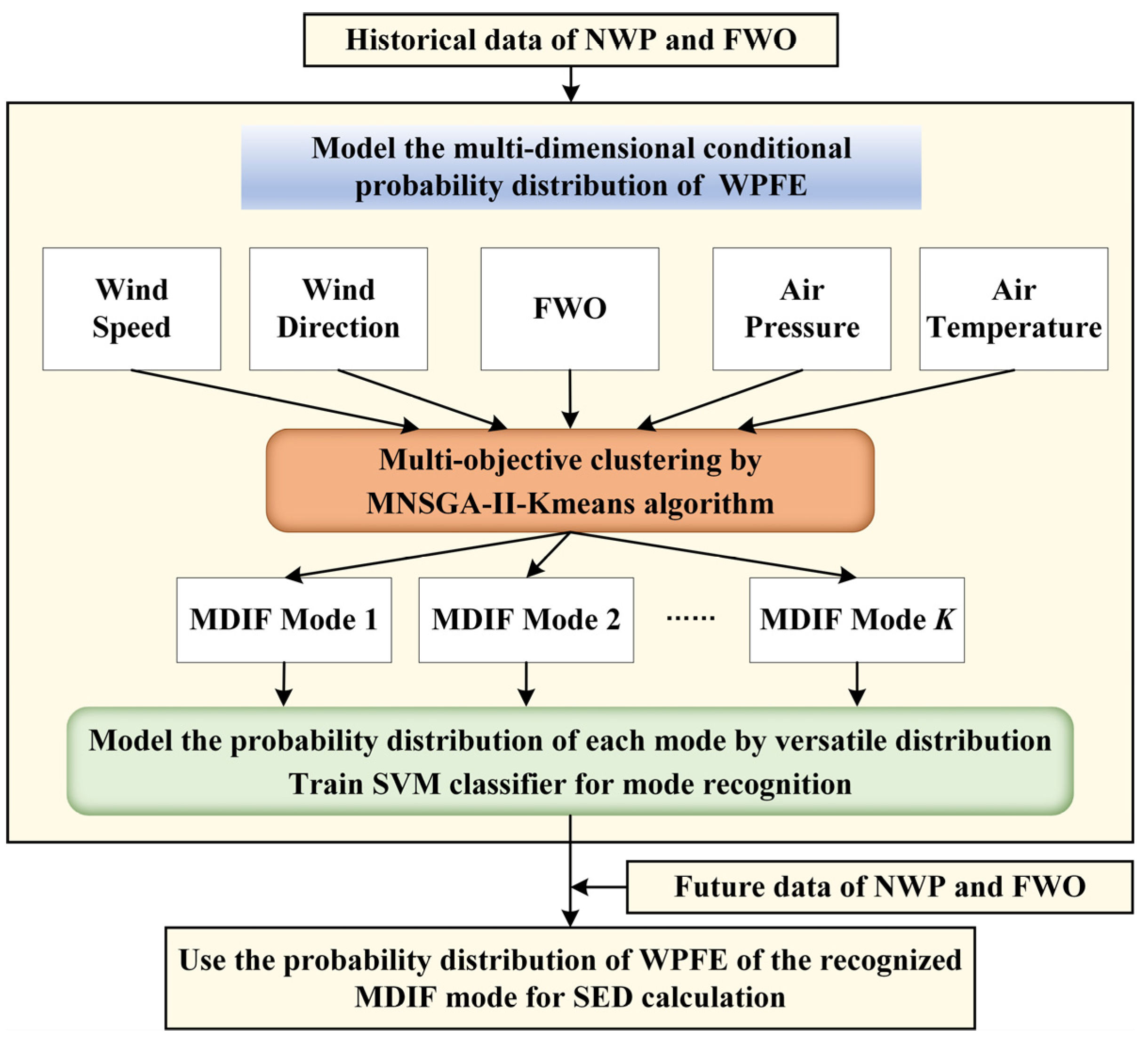
2. Proposed Multi-Dimensional Conditional Probability Distribution Modeling for WPFE

In this paper, the basic idea of establishing and using the multi-dimensional conditional probability distribution of WPFE is summarized as follows:
  • Take the historical data of NWP (wind speed, air temperature, air pressure, etc.) and FWO at the same sampling time to be the historical dataset of MDIF. Then, divide them into several categories by multi-objective clustering algorithm. Each category is called a mode of MDIF. The PDF of historical WPFE data corresponding to each mode is fitted, which is called the conditional probability model of WPFE corresponding to this MDIF mode.
  • The forecast data of MDIF given by NWP and FWO at a certain time in the future are attributed to one of the above-mentioned modes through mode recognition. The PDF of WPFE corresponding to the recognized mode is used as the probability model at the time. Based on the FWO at this time, the probability distribution of wind power is obtained.
The detailed content of the proposed idea is shown in Figure 1. It can be seen that the key to the conditional probability model of WPFE when applied to SED problems is the validity of prior conditions, which are obtained by the clustering of MDIF. If this validity is not considered, it is possible that there is no obvious distinction between the conditional probability models corresponding to different modes. Thus, for SED problems, the idea of conditional probability modeling may not provide substantial help for the final decision.
According to the above analysis, this paper proposes a multi-objective clustering method based on MNSGA-II-Kmeans. This method aims to make the PDF of WPFE corresponding to each MDIF mode have obvious differences, thereby ensuring the effectiveness of prior information for SED problems. In addition, as with the general clustering algorithm, the method also ensures that there is a clear distinction between the clusters of MDIF. Next, how to use MNSGA-II-Kmeans to achieve multi-objective clustering will be introduced in detail.

3. Multi-Objective Clustering Based on MNSGA-II-Kmeans

In the clustering process performed by MNSGA-II-Kmeans, the clustering objects are MDIF, including weather and FWO. Based on the existing research and the correlation analysis between the historical data of WPFE and NWP of an actual wind plant, the wind speed, wind direction, air temperature and air pressure at the height of the hub of the wind turbine are selected as weather factors [12,52,53]. A vector of MDIF is formed from the weather factors and FWO, both taken at the same sampling time. Traditional clustering algorithms, such as Kmeans, only use the distance between samples as a similarity measurement and do not consider the probability distribution characteristics of WDFE of each MDIF mode after clustering. By contrast, the proposed MNSGA-II-Kmeans algorithm can perform multi-objective clustering, thus ensuring that the conditional probability modeling method can provide substantial support for SED problems. The following subsections first introduce the modeling of the multi-objective clustering problem and then introduce the principle of the proposed MNSGA-II-Kmeans algorithm.

3.1. Modeling of Multi-Objective Clustering Problem

The multi-objective clustering model that both considers the clustering effect, as in a traditional clustering algorithm, and the degree of difference in the probability distribution of WPFE after clustering, is presented in Formulas (1)–(8). In the model, the control variables are the clustering centers of each MDIF mode ( O k ).

3.1.1. The Objective Function

The first objective is to minimize the square sum of error (SSE) of clustering samples.
min   SSE
The calculation of SSE is shown in Equation (2), which reflects the degree of aggregation of samples in each MDIF mode. By minimizing the SSE, the samples between each mode can be distinguished by a clear boundary, which can meet the most basic clustering requirements:
SSE = k = 1 K w k , i U k ( w k , i O k ) 2
where K represents the number of MDIF modes, U k represents the sample set of the k th MDIF mode, w represents the vector of MDIF, w k , i represents the i th vector in U k , O k represents the clustering center of U k .
The second objective is to maximize the difference in the probability distribution of WPFE among the MDIF modes after clustering. To quantify the degree of difference of the probability distribution, an index named sum of root mean square error (SRMSE) is proposed. It uses the root mean square error (RMSE) to evaluate the similarity between two probability distributions. The value of it represents the sum of the RMSE between the PDF curves of each MDIF mode in the clustering result. The larger the SRMSE, the higher the degree of difference between the probability distributions. The corresponding minimization objective and the calculation of SRMSE are shown in Formulas (3)–(5):
min SRMSE
SRMSE = i = 1 K 1 j = i + 1 K RMSE ( i , j )
RMSE ( i , j ) = 1 S s = 1 S ( L i , s L j , s ) 2
where RMSE ( i , j ) implies the RMSE calculated from the PDF curve L i of mode i and the PDF curve L j of mode j . L i and L j can be, respectively, obtained from the corresponding historical data of WPFE using KDE. L i , s and L j , s are the probability density values corresponding to the i th same forecast error value of the two PDF curves. S implies the number of sampling points on PDF curves.

3.1.2. Constraints

Equation (6) describes the upper and lower limits of clustering center ( O k ):
w min O k w max
where w min and w max are the minimum and maximum vectors of w , which are composed of the minimum and maximum values of each dimension in w , respectively.
In fact, a mature forecast method usually has high forecast accuracy in most cases. Therefore, to avoid the excessive pursuit of maximizing SRMSE, which may cause the clustering results to be inconsistent with this fact, it is necessary to measure the forecast accuracy of each MDIF mode in the clustering process to ensure that the modes with high accuracy have a larger proportion of samples. Generally, high-precision forecast results often show that the PDF curve of WPFE is narrow and concentrated near 0, while the PDF curve is relatively wide when the accuracy is low, as shown in Figure 2. Accordingly, kurtosis that can reflect the steepness of PDF curve is used to evaluate the forecast accuracy in each mode. The calculation of kurtosis is described in Equation (7).
Kurtosis = 1 h i = 1 h ( Δ p i Δ p ¯ ) 4 ( 1 h i = 1 h ( Δ p i Δ p ¯ ) 2 ) 2
where Δ p is the historical dataset of WPFE belonging to a MDIF mode, h is the number of samples in Δ p , Δ p i is the i th sample, and Δ p ¯ is the average value of Δ p .
Based on the above analysis, this paper uses 3, which is the kurtosis of the standard normal distribution, as the reference value to define an index NK, which represents the proportion of the samples of the models whose kurtosis is greater than 3. In a case where the PDF curve of WPFE has obvious multi-peaks, NK can be obtained by using the actual and forecast wind power data to calculate the forecast accuracy of each mode directly. In this paper, by adding constraint on NK in the multi-objective clustering model, as expressed in Equation (8), the clustering results can meet the requirement that the modes with higher forecast accuracy account for the majority of samples.
NK 60 %

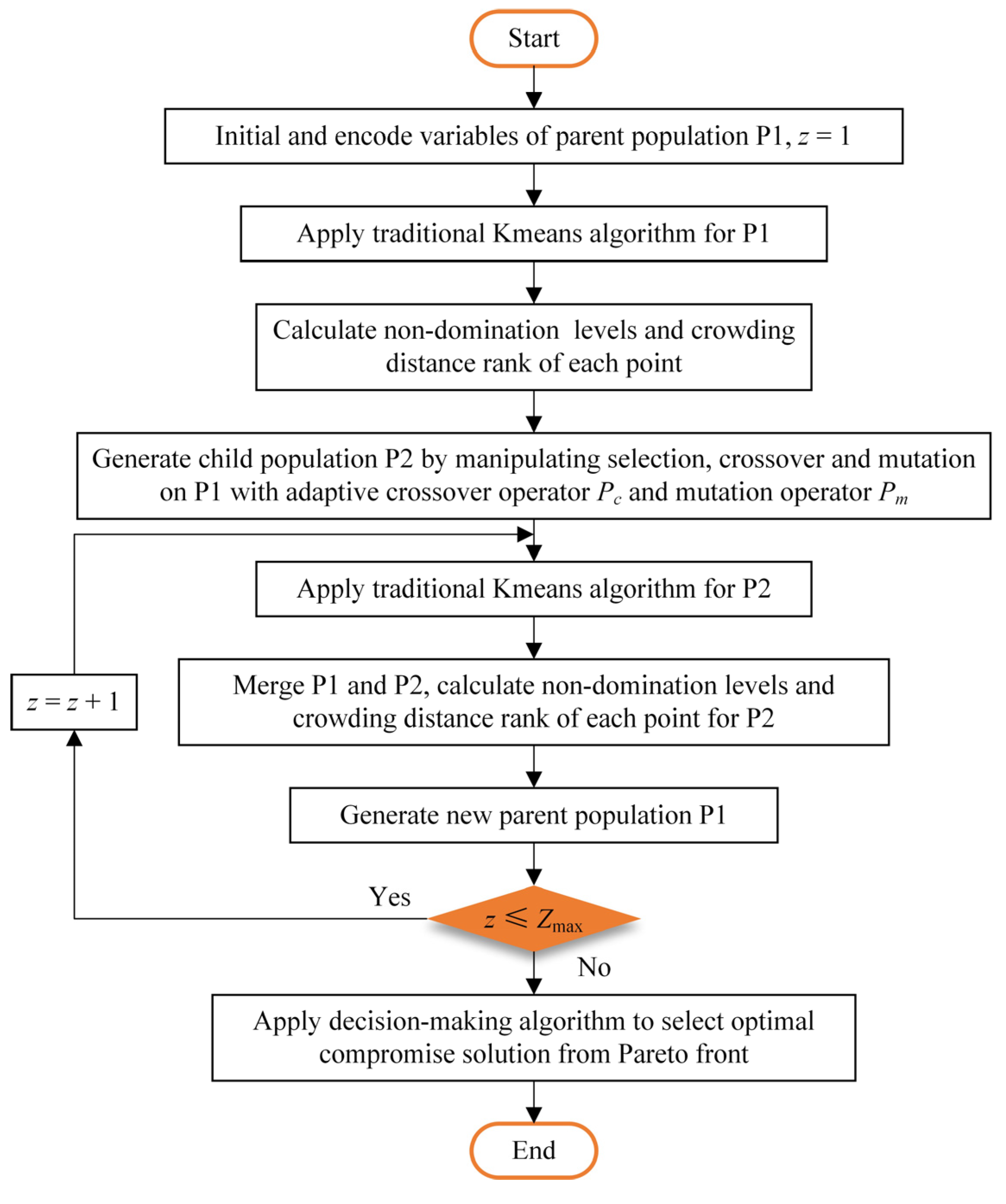
3.2. MNSGA-II-Kmeans Algorithm

The traditional NSGA-II algorithm is a typical algorithm for solving multi-objective problems. However, the fixed crossover rate and mutation rate make it easy for the algorithm to fall into the local optimum. At the same time, when it is directly used to solve the proposed multi-objective clustering problem, the algorithm cannot achieve the clustering of samples. To avoid these problems, the adaptive crossover and mutation operators are proposed, and the Kmeans algorithm is introduced to realize the clustering calculation in the process of multi-objective optimization. The flowchart of the proposed MNSGA-II-Kmeans algorithm is shown in Figure 3. The traditional NSGA-II algorithm mainly includes coding, non-dominated sorting, crowded distance calculation, selection, crossover, mutation and elite preservation strategies. Refer to Ref. [50] for detailed information about the traditional NSGA-II algorithm. Here, we mainly introduce the key technologies. The analysis of the key technology of MNSGA-II-Kmeans is as follows:

3.2.1. Adaptive Crossover Operator and Mutation Operator

The MNSGA-II-Kmeans algorithm uses simulated binary crossover and polynomial mutation. Before performing the cross and mutation operation in each generation, first normalize the objective function of each point, as expressed in Equation (9):
L q p = f q p f q min f q max f q min
where f q p stands for the value of objective q   ( q = 1 , 2 ) at point p , f q max , and f q min stands for the maximum and minimum values of objective q in the current population. L q p is the normalization of f q p .
Taking mutation calculation as an example, to avoid the local optimal and improve the global search ability, individuals with a small objective should be mutated with a small mutation operator, and individuals with a large objective should be mutated with a larger mutation operator on the contrary. The adaptive mutation operator ( P m ) is defined in Equation (10):
P m = { P m 1 ( P m 1 P m 2 ) ( L u , a v g L u ) L u , a v g L u , min ,   L u L ,   L u L u , a v g P m 1 , L > L a v g
where L = [ L 1 , L 2 ] presents the two objectives of the point to be mutated, L a v g = [ L 1 , a v g , L 2 , a v g ] presents the average of the two objectives in the current population, L u presents the objective in L that is less than its average L u , a v g . When L 1 and L 2 are both smaller than their corresponding average, L u presents the objective in L with a greater absolute value of the difference from its average. L u , min presents the minimum value of objective u in the current population. P m 1 and P m 2 are both the mutation rates, and 0 < P m 2 < P m 1 < 1 .
In the crossover operation, for two parent points, calculate L using Equation (11), and replace P m 1 and P m 2 with crossover rates P c 1 and P c 2 , respectively, to obtain the adaptive crossover operator ( P c ).
L = [ min ( L 1 p 1 , L 1 p 2 ) ,   min ( L 2 p 1 , L 2 p 2 ) ]
where L 1 p 1 , L 2 p 1 and L 1 p 2 , L 2 p 2 are the objectives of the parent points p 1 and p 2 , respectively.

3.2.2. Clustering Based on Kmeans Algorithm

Kmeans algorithm is a classic algorithm, which is widely used in big data clustering [54]. It uses Euclidean distance to measure the similarity of samples. By determining K cluster centers, each sample is assigned to the nearest cluster center to achieve sample division, and then the centers are iteratively updated with the objective of minimizing SSE to obtain the final clustering result. Since the Kmeans algorithm is simple, fast and easy to expand [55], the MNSGA-II-Kmeans algorithm uses the global search capability of NSGA-II algorithm to determine the clustering centers and then uses the Kmeans algorithm to obtain the corresponding clustering results. By calculating the objective in the multi-objective clustering problem and iterating continuously, the optimization of the population is realized.
Furthermore, the number of clusters has an intuitive impact on the clustering results. In order to avoid the subjective influence caused by artificially setting the number of clusters, this paper uses the elbow method [56,57] to determine it before the optimization of multi-objective clustering. Reference [56] shows the principle of the elbow method in detail. This method uses Kmeans algorithm to calculate the samples with different number of clusters ( K ) and selects the ideal K according to the inflection point on the SSE-K curve, as shown in Figure 4.

3.2.3. Decision-Making Algorithm

Using the MNSGA-II-Kmeans algorithm, a Pareto front containing non-dominated solutions is obtained. In order to obtain the final optimal compromise solution, the fuzzy satisfactory method is used for selection, as shown in Equations (12) and (13):
L p = max ( L p q )     q = 1 , 2
M = min ( L p )     p = 1 , 2 , , T
where L p implies the maximum value of all objectives of point p in the current Pareto front solution set, M implies the minimum value in the set of L p , T implies the number of points in the Pareto front. The optimal compromise solution of the algorithm is the point corresponding to M .

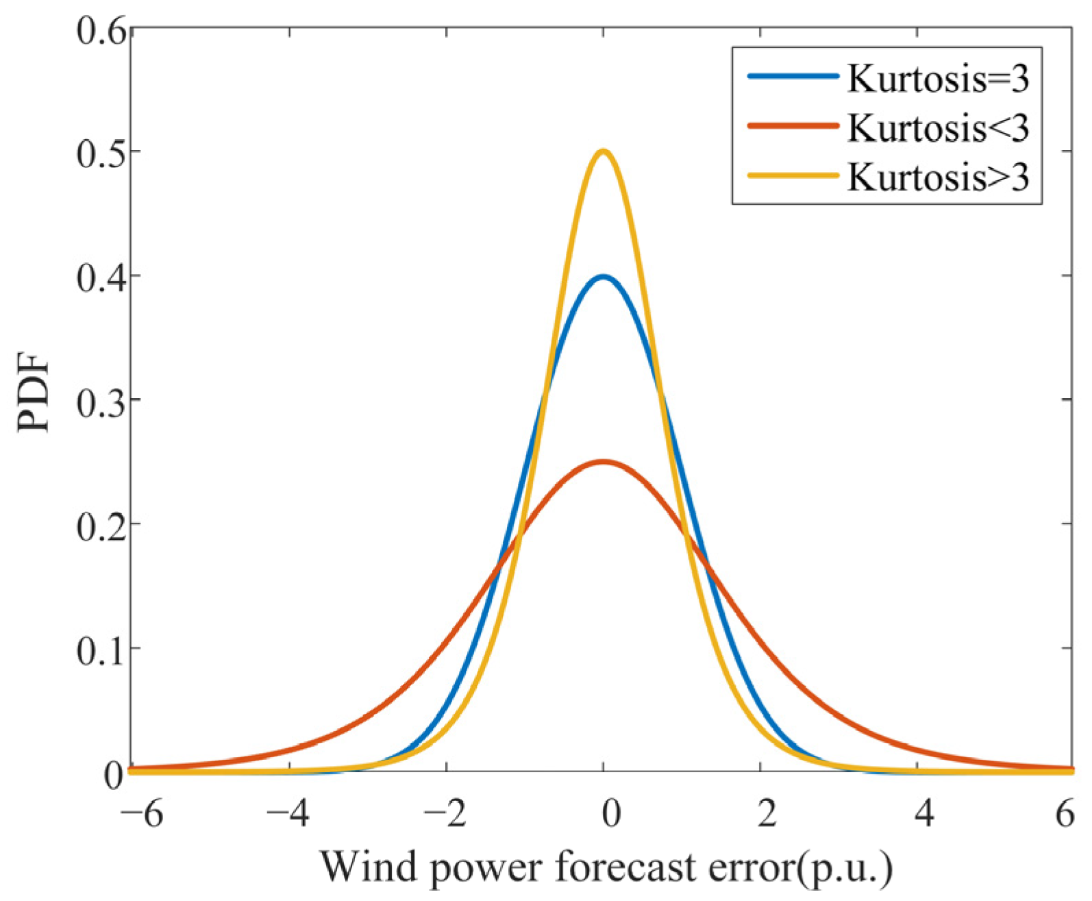
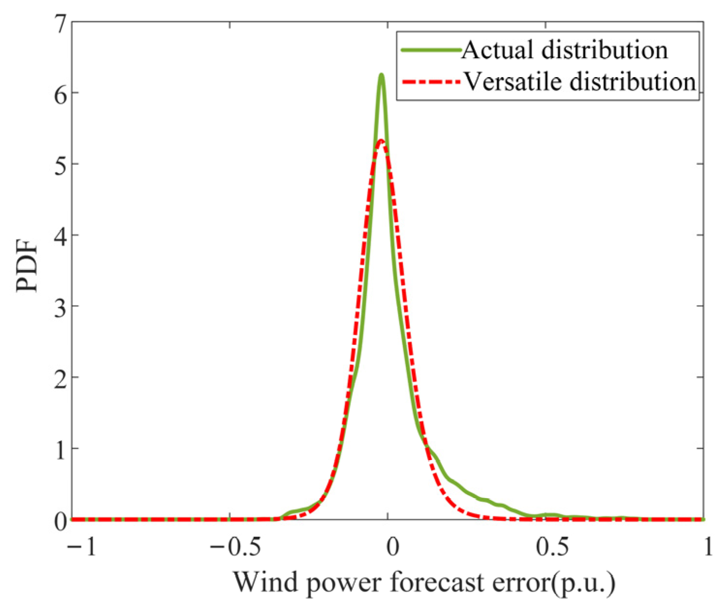
4. Versatile Distribution for Probability Distribution Modeling

After the multi-objective clustering in Section 3, we can obtain WPFE datasets of different MDIF modes and know that there are significant differences between their probability distributions. However, the analytical expression or quantiles of the probability distribution of WPFE for the different MDIF modes, which are necessary for SED, remain unknown. Therefore, it is necessary to further model the probability distribution function of WPFE. In the current research of probability distribution modeling, the KDE method is usually used to obtain the required PDF curve. This method can truly reflect the probability distribution of data and has high accuracy. Nevertheless, the PDF obtained by KDE has no analytical expression, which affects the computational efficiency of SED problems. Therefore, this paper uses the versatile distribution [36] to fit the probability distribution of WPFE of each MDIF mode. Compared with the Gaussian distribution [52] and Beta distribution [58], the versatile distribution can express various probability distributions more accurately. Furthermore, its cumulative distribution function (CDF) is reversible, which is conducive to improving the computational efficiency of SED problems [59]. Equation (14) shows the PDF of versatile distribution:
{ f ( x ) = α β e α ( x γ ) ( 1 + e α ( x γ ) ) β + 1 α > 0 , β > 0 , + > γ >
where α , β and γ are the shape parameters.
Based on Equation (14), the non-linear least square fitting method can be used to obtain the shape parameters of versatile distribution of WPFE. The fitting result is evaluated by the decision coefficient R 2 , and RMSE. Equation (15) shows the calculation of R 2 . A higher accuracy of the fitting result is obtained when R 2 is close to 1 and RMSE is close to 0.
R 2 = 1 i = 1 d ( y i y ^ i ) 2 i = 1 d ( y i y ¯ ) 2
where y i represents the value of points to be fitted, y ^ i represents the fitting value of y i , y ¯ represents the average of y i , d represents the number of points to be fitted.

5. SVM Algorithm for Mode Recognition

Based on the MDIF modes obtained by clustering and the corresponding versatile distribution of WPFE, in practical application, it is necessary to accurately classify the data of NWP and FWO at a certain time in the future, so as to select the corresponding conditional probability model of WPFE for SED calculation. Considering the high efficiency of SVM algorithm in non-linear classification of high-dimensional data, such as weather data, this paper uses SVM algorithm to perform mode recognition on MDIF [60,61,62].
SVM is a machine-learning method based on statistical learning theories, such as the Vapnik–Chervonenkis (VC) dimension and structure risk minimization principle (SRM). It transforms the input vector into a high-dimensional feature space using the kernel function and achieves data classification by constructing an optimal separation hyperplane. The following improvements are applied in this paper:
  • Use a one-against-one method [63,64] to deal with the situation when the number of MDIF modes is greater than 2. This is because a single SVM classifier can only solve the classification of two categories.
  • Select the RBF kernel function that performs better in most cases.
  • Optimize the main influencing parameters of SVM, such as penalty factor ( C ) and kernel function parameter ( g ), using grid search and 3-fold cross validation [65,66]. This can improve the classification accuracy effectively.
  • Equation (16) shows how to calculate the accuracy of SVM classification.
a c c u r a c y = n 1 n 2
where n 1 represents the number of samples correctly classified by SVM, n 2 represents the number of samples that were classified.

6. Experimental Results

In order to verify the effectiveness of the proposed method, the historical data of WPFE and MDIF from a wind plant in north China are used for the case study. The capacity of the wind plant is 49.5 MW, and the data were sampled every 15 min in the period from 1 January 2019 to 31 December 2019. All data are normalized and divided into training set and testing set randomly, with a ratio of 8:2. Due to the obvious differences in weather and wind power between seasons, the clustering of MDIF and the modeling of WPFE are performed on the data subset of each season for more accurate results.

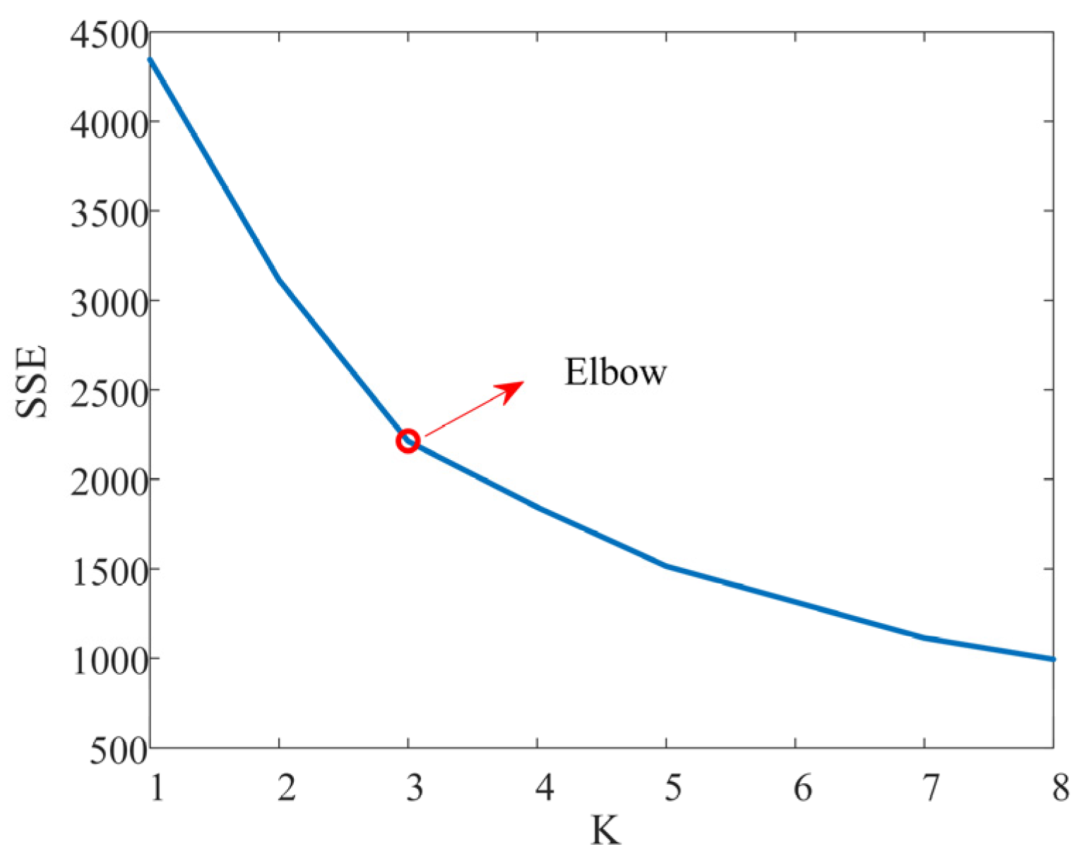
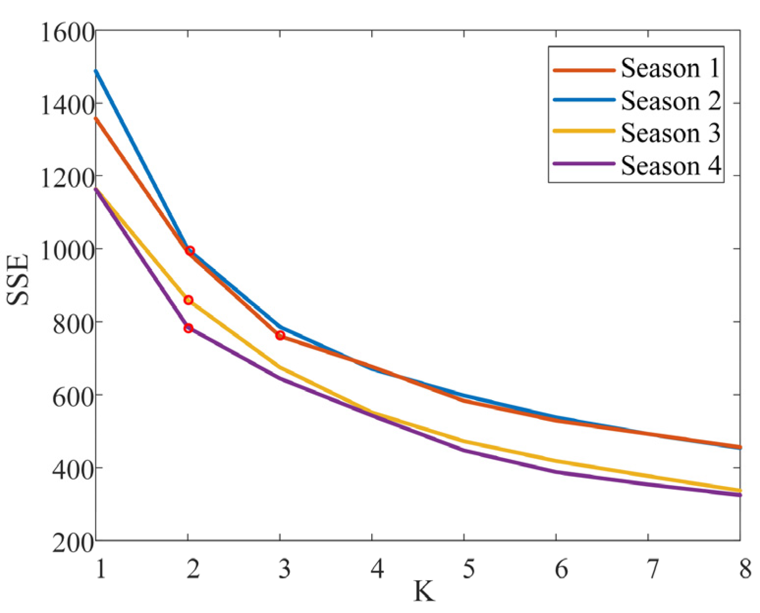
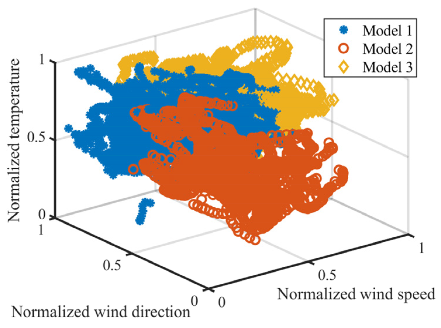
6.1. Multi-Objective Clustering Results

Before performing the multi-objective clustering of MDIF, the elbow method is used to determine the number of MDIF modes of each season in historical training data. Figure 5 shows the SSE-K curves, where season 1, season 2, season 3 and season 4 represent spring, summer, autumn and winter, respectively. The results show that the number of MDIF modes for each season are 3, 2, 2, 2, which means there are 9 modes in total.
Based on the obtained number of MDIF modes, the MSNGA-II-Kmeans algorithm is used to solve the multi-objective clustering problem. In this case, set the initial population number to 50, the maximum number of iterations Zmax = 300, the crossover rates P c 1 = 0.9 , P c 2 = 0.5 , and the mutation rates P m 1 = 0.1 , P m 2 = 0.001 . Take the results of season 1 for display. Figure 6 shows the Pareto front solution set of season 1. Figure 7 shows the clustering results of MDIF data in season 1. It can be seen that there are obvious boundaries between the samples of each mode. Figure 8a shows the PDF curves of WPFE corresponding to each mode of season 1. Obviously, there are differences in the probability distribution of WPFE of each MDIF mode. To further verify the advantages of the proposed MNSGA-II-Kmeans algorithm in making the probability distribution of WPFE of each MDIF mode have obvious difference, the traditional Kmeans algorithm is used to cluster with the same K and same samples. The PDF curves of WPFE of each MDIF mode in season 1 obtained by Kmeans algorithm are shown in Figure 8b. Table 1 shows the comparison of the clustering results of Kmeans algorithm and the proposed MNSGA-II-Kmeans algorithm.
From Table 1 and Figure 8, it can be seen that the SRMSE of each season obtained by MNSGA-II-Kmeans is better than those obtained by Kmeans. The difference between the SRMSE obtained by the two algorithms, respectively, in season 1, is the largest, i.e., 2.7899 obtained by MNSGA-II-Kmeans and 2.0424 obtained by Kmeans. This indicates that the multi-objective clustering based on MNSGA-II-Kmeans can obtain the MDIF clustering results with the largest difference in the probability distribution of WPFE of each mode. Although the clustering result obtained by MNSGA-II-Kmeans corresponds to a larger SSE, this is equivalent to sacrificing part of the clustering effect in exchange for better probability distribution characteristics of WPFE. In addition, NK of each season obtained by the proposed method is greater than 60%, of which the highest is 78.02% in season 1. However, NK of each season obtained by the Kmeans algorithm is below 60%, and the lowest is 24.32% in season 2. It can be concluded that the proposed MNSGA-II-Kmeans algorithm can ensure that the clustering results meet the statistical requirement, that is, the samples corresponding to the MDIF mode with high forecast accuracy account for the majority.

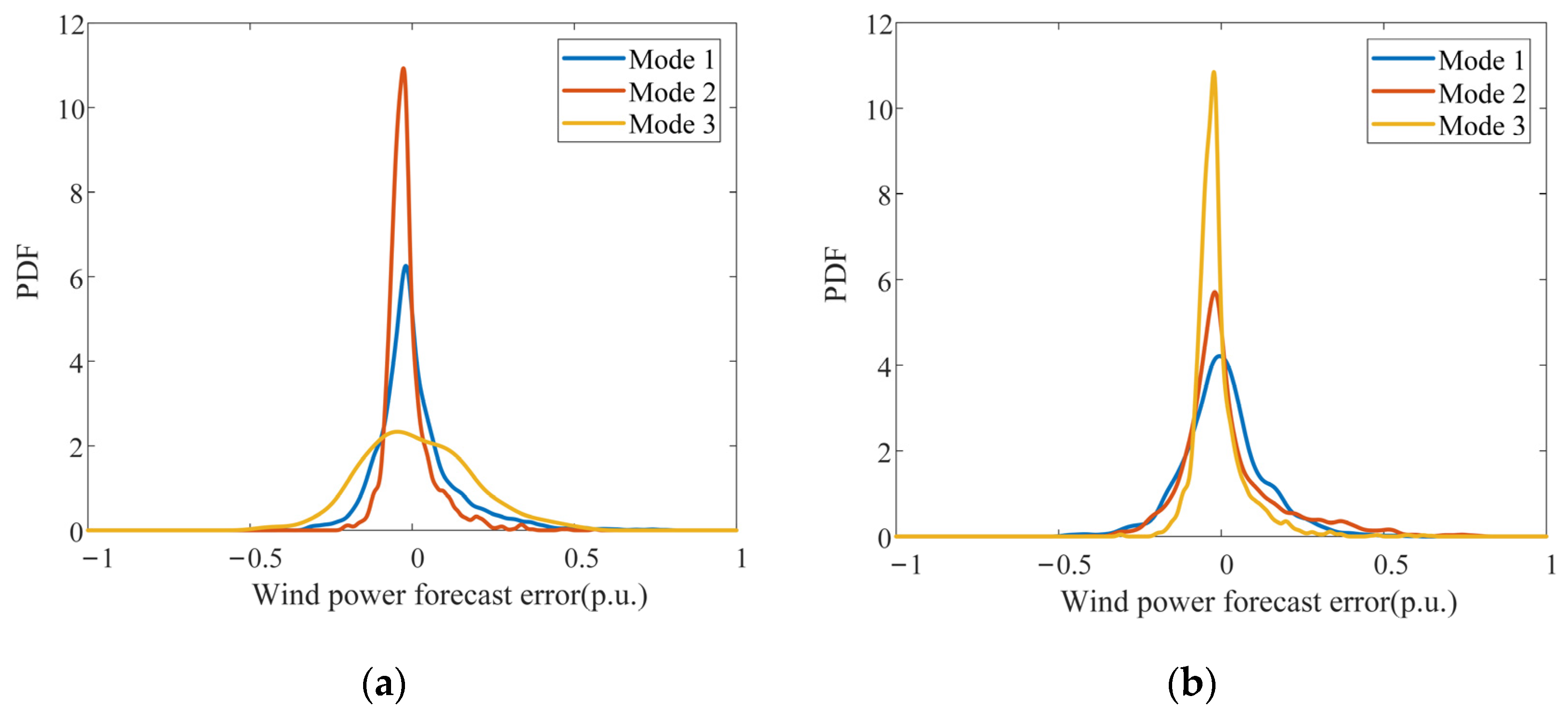
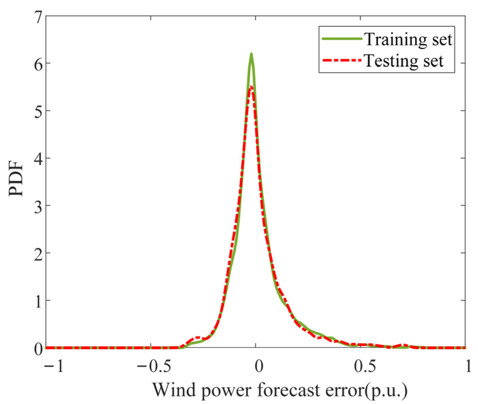
6.2. Results of Probability Distribution Modeling

Based on the obtained PDF curves of WPFE of each MDIF mode, the final multi-dimensional conditional probability model of WPFE can be obtained using the versatile distribution and non-linear least square fitting method. Table 2 shows the modeling and evaluation results of versatile distribution of each MDIF mode in each season. Figure 9 compares the PDF curve of versatile distribution of WPFE in season 1, mode 1, with the actual PDF curve.
The above results show that R 2 is greater than 0.9, and RMSE is less than 0.3 in each season, which indicates that the versatile distribution can well represent the probability distribution of WPFE. Meanwhile, the good analyticity of the versatile distribution is conducive to the calculation of SED problems, considering the randomness of wind power.

6.3. Verification of MDIF Mode Recognition

To train and verify the SVM classifier, the training set is further divided into sub-training set and sub-testing set according to 8:2. When using grid search and 3-fold cross validation to optimize SVM parameters, set the change range of C and g to 2−3 to 27, and the change step to 20.5. This is to avoid poor generalization ability of training results caused by overfitting or low recognition accuracy caused by less fitting. Table 3 lists the SVM parameters optimization results, the optimal recognition accuracy of each season after optimization and the recognition accuracy of each season verified by the sub-testing set.
It is clear from Table 3 that the SVM recognition accuracy verified by the sub-testing set in each season is above 99%. Therefore, in actual applications, the SVM classifier can meet the needs of accurately identifying the MDIF mode based on NWP and FWO. Use the SVM classifier obtained to classify the initial testing set into each MDIF mode and calculate the PDF curve of each mode. The PDF curves of WPFE corresponding to mode 1 of season 1 in the initial training set and the initial testing set are shown in Figure 10. It can be observed that the probability distributions of WPFE of the training data and the testing data in the same mode are highly consistent, which indicates that the obtained results of clustering and probability distribution modeling by the proposed method are applicable. It is worth noting that, since SVM is a sample-based machine-learning algorithm, its higher recognition accuracy depends on the given samples. Therefore, after a certain period of data accumulation, it is necessary to update the dataset and repeat the clustering, modeling and training process mentioned in Section 2, Section 3, Section 4 and Section 5 to ensure the accuracy and timeliness of the modeling results and the SVM models.

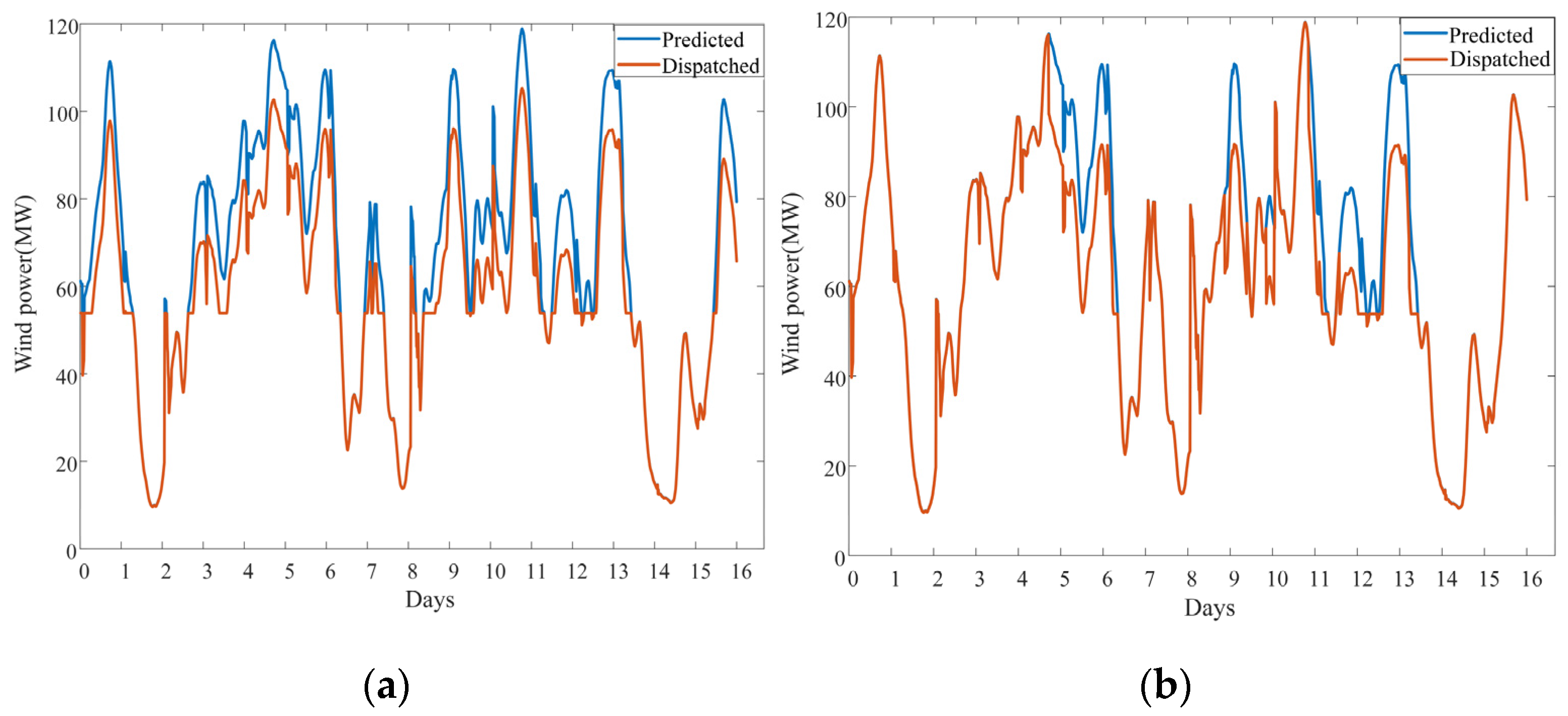
6.4. Application in SED Problems

This paper further uses a simple SED problem considering the uncertainty of wind power to illustrate the effectiveness of the proposed method for improving the consumption capacity of wind power of the power system. In the SED problem, the obtained multi-dimensional conditional probability models of WPFE are compared with the probability model obtained by simply fitting the probability distribution of all the historical WPFE data without considering conditional information. The SED problem used is an idealized single time section stochastic optimal power flow problem, as shown in Equation (17):
{ min m = 1 N 1 ( a m P M , m 2 + b m P M , m + c m ) s . t . P M , m min P M , m P M , m max 0 R M , m P M , m max 10 % P M , m + R M , m P M , m max 0 P W , i P W , i p r e i = 1 N 2 ( P W , i P W , i v , d o w n ) m = 1 N 1 R M , m i = 1 N 2 P W , i + m = 1 N 1 P M , m = P L
where a m , b m and c m represent the fuel cost coefficients of thermal unit m , N 1 is the number of thermal units, P M , m is the power output of thermal unit m , P M , m min and P M , m max are the minimum and maximum values of the power output of thermal unit m , R M , m stands for the power reserve of thermal unit m . P W , i presents the dispatched power of wind plant i , P W , i p r e presents the FWO of wind plant i . P W , i v , d o w n is the lower limit of the possible wind power output at the confidence level v , which can be obtained by superimposing the quantile of the probability distribution of WPFE on P W , i p r e . N 2 is the number of wind plants, and P L is the load of the power system.
In other words, this problem is to determine the output of thermal units to achieve the lowest fuel cost based on the lower limits of the possible wind power output at a certain confidence level, i.e., to consume as much wind power as possible. It is obvious that the lower the thermal power output of the decision, the higher the wind power output. In this way, the gap between the dispatched wind power and the above-mentioned lower limits increases. It may not be possible to meet the constraint that the maximum reserve of thermal units should be greater than this gap, which in turn may lead to load shedding. Therefore, the wind power consumption in this SED problem is highly dependent on the estimation of the lower limits of possible wind power output at a high confidence level. This is closely related to the research of this paper on the modeling of the probability distribution of WPFE.
A system composed of one wind plant and six thermal units is used for the calculation of the proposed SED problem. The parameters of thermal units are shown in Table A1 in the Appendix A. The wind plant previously used for clustering and modeling is chosen to be the wind plant in this system with rescaled capacity. The confidence level is 0.95. Based on the historical data of NWP and FWO, the stochastic optimal power flow calculation is performed every 15 min over 16 days, for a total of 1536 times. Figure 11 and Table 4 show the results of the proposed SED problem using the two probability distribution modeling methods. It is clear that applying the non-conditional probability model of WPFE, which does not consider MDIF, the dispatched wind power is significantly lower than the forecast value when the latter is high. The reason is the lower limits of possible wind power output obtained by this model are relatively low, and the thermal power reserve is insufficient. Thus, the system has to reduce the dispatched wind power to avoid load shedding. In this case, the actual wind power consumption of the system is 22,370.23 MWh. When the obtained SVM classifier is used for mode recognition, and the proposed multi-dimensional conditional probability models of WPFE are used for calculation, the dispatched wind power is the same as the forecast value for most of the times. This is because after adopting the multi-dimensional conditional probability models, the lower limit of possible wind power output is closer to the forecast value at these times. That is, the uncertainty information of wind power is more accurate. Hence, the system can consume wind power as much as possible without excessive thermal power reserve. In this case, the actual wind power consumption of the system is 23,765.15 MWh, an increase of 1394.92 MWh.
In order to further illustrate the reliability of the estimated lower limit of possible wind power output, we introduced the actual values of wind power at the calculated moments as a comparison and defined the lower limit coverage rate (LLCR) to indicate the probability that the actual value is above the estimated lower limit. It can be seen that the higher the LLCR is, the higher the reliability of the estimated lower limits is. Table 4 shows the LLCR when using the two models, respectively. It is clear that the LLCR of the non-conditional probability model of WPFE is higher. However, this is because it does not perform the conditional modeling proposed in this paper, and thus, the lower limits that it estimates are lower. Moreover, the difference between the LLCR corresponding to the two models is small, and both are above 96%, i.e., the lower limits they estimated both have high reliability. On this basis, excluding the case where the lower limits estimated by the two models are both 0 due to the low FWO, the proportion of the times with better lower limit estimated by the proposed method is 75.98%. What a better lower limit means is that it is closer to the forecast value. The above results show that the proposed method has higher modeling accuracy for probability distribution of WPFE, and the result that the wind power consumption of the system can be increased is true and reliable.
In summary, the proposed method of probability distribution modeling of multi-dimensional conditions for WPFE based on MNSGA-II-Kmeans ensures the validity of the conditional probability distribution for SED problems. Therefore, it improves the wind power consumption ability of the power system from a statistical point of view.

7. Conclusions

This paper considered both the influence of weather and FWO on the probability distribution of WPFE and proposed a method of probability distribution modeling of multi-dimensional conditions for WPFE based on MNSGA-II-Kmeans. Based on the traditional clustering algorithm, this method added the degree of difference between the probability distribution of WPFE in different conditions as one of the objectives to perform multi-objective clustering. The case study based on actual historical data of a wind plant in north China verified the effectiveness of the method.
The value of conditional probability modeling of WPFE for SED problems lies in the significant difference between probability distributions under different conditions. The results show that the multi-objective clustering based on the proposed MNSGA-II-Kmeans algorithm can accurately obtain the clustering result with the largest difference between the probability distributions of WPFE of each mode. Moreover, the existing mature forecast methods have high forecast accuracy most of the time, but poor forecast accuracy during extreme weather, which indicates the necessity of clustering MDIF data from the perspective of the difference in probability distribution of WPFE. As a result of this work, by using the probability distribution of WPFE of different MDIF modes according to the situation in SED problems, the wind power consumption of the power system can be effectively increased from a statistical point of view.
Future work will focus on considering the impact of more complex environmental factors on WPFE, such as wind turbulence and uncertainty of weather factors, improving the modeling accuracy of the probability distribution of WPFE and proposing a probability distribution modeling method for wind farm cluster. Moreover, how to combine the proposed method with the wind power probabilistic prediction method will also be studied in future.

Author Contributions

Conceptualization, J.Y. and Y.L. (Yu Liu); methodology, S.J.; software, N.L.; validation, J.Y. and D.K.; investigation, Y.L. (Yu Liu); resources, Y.L. (Yazhou Luo); data curation, S.J.; writing—review and editing, N.L.; visualization, N.L.; supervision, D.K. All authors have read and agreed to the published version of the manuscript.

Funding

This research was funded by State Grid Corporation of China (520101180052).

Institutional Review Board Statement

Not applicable.

Informed Consent Statement

Not applicable.

Data Availability Statement

Not applicable.

Conflicts of Interest

The authors declare no conflict of interest.

Abbreviations

The following abbreviations are used in this manuscript:
VMDVariational mode decomposition
LSTMLong short-term memory network
EMDEmpirical mode decomposition
SWDStationary wavelet decomposition
ANFISArtificial neuro-fuzzy inference system
ANNArtificial neural network
SVRSupport vector regression
WPFEWind power forecast error
MDIFMulti-dimensional influencing factors
SVMSupport vector machine
NWPNumerical weather prediction
PDFProbability density function
FWOForecast wind power output
SEDStochastic economic dispatch
PAESPareto-archived evolution strategy
SPEAStrength Pareto evolutionary algorithm
SSESquare sum of error
SRMSESum of root mean square error
RMSERoot mean square error
KDEKernel density estimation
VCVapnik–Chervonenkis
SRMStructure risk minimization principle
CDFCumulative distribution function
LLCRLower limit coverage rate

Appendix A

Table A1. Parameters of thermal units.
UnitCapacitya
($/MW2)
b
($/MW)
c
($)
Minimum
Output
Maximum
Output
#1 1, #2, #3100 MW0.05342781100 MW35 MW
#4, #5, #680 MW0.0144321280 MW28 MW
1 #1 means the first thermal unit in the proposed system, same as #2–#6.

References

  1. Jiang, R.; Wang, J.; Guan, Y. Robust Unit Commitment With Wind Power and Pumped Storage Hydro. IEEE Trans. Power Syst. 2012, 27, 800–810. [Google Scholar] [CrossRef]
  2. Bertsimas, D.; Litvinov, E.; Sun, X.A.; Zhao, J.; Zheng, T. Adaptive Robust Optimization for the Security Constrained Unit Commitment Problem. IEEE Trans. Power Syst. 2013, 28, 52–63. [Google Scholar] [CrossRef]
  3. Dvorkin, Y.; Lubin, M.; Backhaus, S.; Chertkov, M. Uncertainty Sets for Wind Power Generation. IEEE Trans. Power Syst. 2016, 31, 3326–3327. [Google Scholar] [CrossRef] [Green Version]
  4. Yu, H.; Chung, C.Y.; Wong, K.P.; Zhang, J.H. A Chance Constrained Transmission Network Expansion Planning Method With Consideration of Load and Wind Farm Uncertainties. IEEE Trans. Power Syst. 2009, 24, 1568–1576. [Google Scholar] [CrossRef]
  5. Wang, Y.; Zhang, N.; Kang, C.; Miao, M.; Shi, R.; Xia, Q. An Efficient Approach to Power System Uncertainty Analysis With High-Dimensional Dependencies. IEEE Trans. Power Syst. 2018, 33, 2984–2994. [Google Scholar] [CrossRef]
  6. Le, X.; Yingzhong, G.; Xinxin, Z.; Genton, M. Short-term spatio-temporal wind power forecast in robust look-ahead power system dispatch. In Proceedings of the 2016 IEEE Power and Energy Society General Meeting (PESGM), Boston, MA, USA, 17–21 July 2016. [Google Scholar] [CrossRef]
  7. Li, Y.; Wang, Y.; Wu, B. Short-Term Direct Probability Prediction Model of Wind Power Based on Improved Natural Gradient Boosting. Energies 2020, 13, 4629. [Google Scholar] [CrossRef]
  8. Buhan, S.; Özkazanç, Y.; Çadırcı, I. Wind Pattern Recognition and Reference Wind Mast Data Correlations With NWP for Improved Wind-Electric Power Forecasts. IEEE Trans. Ind. Inform. 2016, 12, 991–1004. [Google Scholar] [CrossRef]
  9. Tascikaraoglu, A.; Uzunoglu, M. A review of combined approaches for prediction of short-term wind speed and power. Renew. Sustain. Energy Rev. 2014, 34, 243–254. [Google Scholar] [CrossRef]
  10. Jung, J.; Broadwater, R.P. Current status and future advances for wind speed and power forecasting. Renew. Sustain. Energy Rev. 2014, 31, 762–777. [Google Scholar] [CrossRef]
  11. Wang, J.; Hu, J.; Ma, K.; Zhang, Y. A self-adaptive hybrid approach for wind speed forecasting. Renew. Energy 2015, 78, 374–385. [Google Scholar] [CrossRef]
  12. Li, D.; Yan, W.; Li, W.; Ren, Z. A Two-Tier Wind Power Time Series Model Considering Day-to-Day Weather Transition and Intraday Wind Power Fluctuations. IEEE Trans. Power Syst. 2016, 31, 4330–4339. [Google Scholar] [CrossRef]
  13. Shi, Z.; Liang, H.; Dinavahi, V. Direct Interval Forecast of Uncertain Wind Power Based on Recurrent Neural Networks. IEEE Trans. Sustain. Energy 2018, 9, 1177–1187. [Google Scholar] [CrossRef]
  14. Han, L.; Zhang, R.; Wang, X.; Bao, A.; Jing, H. Multi-step wind power forecast based on VMD-LSTM. IET Renew. Power Gener. 2019, 13, 1690–1700. [Google Scholar] [CrossRef]
  15. Cevik, H.H.; Cunka, M.; Polat, K. A new multistage short-term wind power forecast model using decomposition and artificial intelligence methods. Phys. A Stat. Mech. Appl. 2019, 534, 122177. [Google Scholar] [CrossRef]
  16. Bibi, N.; Shah, I.; Alsubie, A.; Ali, S.; Lone, S.A. Electricity Spot Prices Forecasting Based on Ensemble Learning. IEEE Access 2021, 9, 150984–150992. [Google Scholar] [CrossRef]
  17. Lisi, F.; Shah, I. Forecasting next-day electricity demand and prices based on functional models. Energy Syst. 2020, 11, 947–979. [Google Scholar] [CrossRef]
  18. Shah, I.; Lisi, F. Day-Ahead Electricity Demand Forecasting with Nonparametric Functional Models. In Proceedings of the 12th International Conference on the European Energy Market, EEM 2015, Lisbon, Portugal, 19–22 May 2015; IEEE Computer Society: Lisbon, Portugal, 2015; pp. 1–5. [Google Scholar] [CrossRef]
  19. Shah, I.; Lisi, F. Forecasting of electricity price through a functional prediction of sale and purchase curves. J. Forecast. 2020, 39, 242–259. [Google Scholar] [CrossRef]
  20. Liu, R.; Peng, M.; Xiao, X. Ultra-Short-Term Wind Power Prediction Based on Multivariate Phase Space Reconstruction and Multivariate Linear Regression. Energies 2018, 11, 2763. [Google Scholar] [CrossRef] [Green Version]
  21. Zhang, Y.; Wang, J.; Wang, X. Review on probabilistic forecasting of wind power generation. Renew. Sustain. Energy Rev. 2014, 32, 255–270. [Google Scholar] [CrossRef]
  22. Shouman, N.; Hegazy, Y.G.; Omran, W.A. Hybrid Mean Variance Mapping Optimization Algorithm for Solving Stochastic Based Dynamic Economic Dispatch Incorporating Wind Power Uncertainty. Electr. Power Compon. Syst. 2021, 48, 1786–1797. [Google Scholar] [CrossRef]
  23. Hu, Z.; Xu, Y.; Korkali, M.; Chen, X.; Mili, L.; Valinejad, J. A Bayesian Approach for Estimating Uncertainty in Stochastic Economic Dispatch Considering Wind Power Penetration. IEEE Trans. Sustain. Energy 2021, 12, 671–681. [Google Scholar] [CrossRef]
  24. Wang, X.; Liu, R.-P.; Wang, X.; Hou, Y.; Bouffard, F. A Data-Driven Uncertainty Quantification Method for Stochastic Economic Dispatch. IEEE Trans. Power Syst. 2022, 37, 812–815. [Google Scholar] [CrossRef]
  25. Zeng, L.; Xu, J.; Liu, Y.; Li, C.; Wu, M.; Wen, M.; Xiao, H. Stochastic economic dispatch strategy based on quantile regression. Int. J. Electr. Power Energy Syst. 2022, 134, 107363. [Google Scholar] [CrossRef]
  26. Tang, C.; Xu, J.; Sun, Y.; Liu, J.; Ma, X.; Jiang, H. Stochastic dynamic economic dispatch with multiple wind farms based on wind power conditional distribution models. In Proceedings of the 2017 IEEE Power and Energy Society General Meeting, PESGM 2017, Chicago, IL, USA, 16–20 July 2017; IEEE Computer Society: Chicago, IL, USA, 2018; pp. 1–5. [Google Scholar] [CrossRef]
  27. Bludszuweit, H.; Dominguez-Navarro, J.A.; Llombart, A. Statistical analysis of wind power forecast error. IEEE Trans. Power Syst. 2008, 23, 983–991. [Google Scholar] [CrossRef]
  28. Ge, F.; Ju, Y.; Qi, Z.; Lin, Y. Parameter estimation of a Gaussian mixture model for wind power forecast error by riemann L-BFGS optimization. IEEE Access 2018, 6, 38892–38899. [Google Scholar] [CrossRef]
  29. Yu, Y.; Yang, M.; Han, X.; Zhang, Y.; Ye, P. A Regional Wind Power Probabilistic Forecast Method Based on Deep Quantile Regression. IEEE Trans. Ind. Appl. 2021, 57, 4420–4427. [Google Scholar] [CrossRef]
  30. Zhou, Y.; Sun, Y.; Wang, S.; Mahfoud, R.J.; Alhelou, H.H.; Hatziargyriou, N.; Siano, P. Performance Improvement of Very Short-term Prediction Intervals for Regional Wind Power Based on Composite Conditional Nonlinear Quantile Regression. J. Mod. Power Syst. Clean Energy 2022, 10, 60–70. [Google Scholar] [CrossRef]
  31. Dong, W.; Sun, H.; Tan, J.; Li, Z.; Zhang, J.; Yang, H. Regional wind power probabilistic forecasting based on an improved kernel density estimation, regular vine copulas, and ensemble learning. Energy 2022, 238, 122045. [Google Scholar] [CrossRef]
  32. Yang, X.; Ma, X.; Kang, N.; Maihemuti, M. Probability Interval Prediction of Wind Power Based on KDE Method with Rough Sets and Weighted Markov Chain. IEEE Access 2018, 6, 51556–51565. [Google Scholar] [CrossRef]
  33. Wang, J.; Niu, T.; Lu, H.; Yang, W.; Du, P. A Novel Framework of Reservoir Computing for Deterministic and Probabilistic Wind Power Forecasting. IEEE Trans. Sustain. Energy 2020, 11, 337–349. [Google Scholar] [CrossRef]
  34. Lin, Y.; Yang, M.; Wan, C.; Wang, J.; Song, Y. A Multi-Model Combination Approach for Probabilistic Wind Power Forecasting. IEEE Trans. Sustain. Energy 2019, 10, 226–237. [Google Scholar] [CrossRef]
  35. Bruninx, K.; Delarue, E. A Statistical Description of the Error on Wind Power Forecasts for Probabilistic Reserve Sizing. IEEE Trans. Sustain. Energy 2014, 5, 995–1002. [Google Scholar] [CrossRef]
  36. Zhang, Z.; Sun, Y.; Gao, D.W.; Lin, J.; Cheng, L. A Versatile Probability Distribution Model for Wind Power Forecast Errors and Its Application in Economic Dispatch. IEEE Trans. Power Syst. 2013, 28, 3114–3125. [Google Scholar] [CrossRef]
  37. Jia, M.; Shen, C.; Wang, Z. A Distributed Probabilistic Modeling Algorithm for the Aggregated Power Forecast Error of Multiple Newly Built Wind Farms. IEEE Trans. Sustain. Energy 2019, 10, 1857–1866. [Google Scholar] [CrossRef]
  38. Tang, C.; Xu, J.; Sun, Y.; Liu, J.; Li, X.; Ke, D.; Yang, J.; Peng, X. Look-Ahead Economic Dispatch With Adjustable Confidence Interval Based on a Truncated Versatile Distribution Model for Wind Power. IEEE Trans. Power Syst. 2018, 33, 1755–1767. [Google Scholar] [CrossRef]
  39. Gómez-Lázaro, E.; Bueso, M.C.; Kessler, M.; Martín-Martínez, S.; Zhang, J.; Hodge, B.-M.; Molina-García, A. Probability Density Function Characterization for Aggregated Large-Scale Wind Power Based on Weibull Mixtures. Energies 2016, 9, 91. [Google Scholar] [CrossRef] [Green Version]
  40. Pinson, P.; Kariniotakis, G. Conditional Prediction Intervals of Wind Power Generation. IEEE Trans. Power Syst. 2010, 25, 1845–1856. [Google Scholar] [CrossRef] [Green Version]
  41. Zhang, N.; Kang, C.; Xia, Q.; Liang, J. Modeling Conditional Forecast Error for Wind Power in Generation Scheduling. IEEE Trans. Power Syst. 2014, 29, 1316–1324. [Google Scholar] [CrossRef]
  42. Wang, Z.; Shen, C.; Liu, F. A conditional model of wind power forecast errors and its application in scenario generation. Appl. Energy 2018, 212, 771–785. [Google Scholar] [CrossRef] [Green Version]
  43. Ela, E.; O’Malley, M. Studying the Variability and Uncertainty Impacts of Variable Generation at Multiple Timescales. IEEE Trans. Power Syst. 2012, 27, 1324–1333. [Google Scholar] [CrossRef] [Green Version]
  44. Khorramdel, B.; Chung, C.Y.; Safari, N.; Price, G.C.D. A Fuzzy Adaptive Probabilistic Wind Power Prediction Framework Using Diffusion Kernel Density Estimators. IEEE Trans. Power Syst. 2018, 33, 7109–7121. [Google Scholar] [CrossRef]
  45. Sorensen, P.; Cutululis, N.A.; Vigueras-Rodriguez, A.; Madsen, H.; Pinson, P.; Jensen, L.E.; Hjerrild, J.; Donovan, M. Modelling of power fluctuations from large offshore wind farms. Wind Energy 2008, 11, 29–43. [Google Scholar] [CrossRef]
  46. Xie, W.; Zhang, P.; Chen, R.; Zhou, Z. A Nonparametric Bayesian Framework for Short-Term Wind Power Probabilistic Forecast. IEEE Trans. Power Syst. 2019, 34, 371–379. [Google Scholar] [CrossRef]
  47. Su, X.; Masoum, M.A.S.; Wolfs, P.J. Optimal PV Inverter Reactive Power Control and Real Power Curtailment to Improve Performance of Unbalanced Four-Wire LV Distribution Networks. IEEE Trans. Sustain. Energy 2014, 5, 967–977. [Google Scholar] [CrossRef]
  48. Wu, X.; Shi, W.; Du, J. Multi-Objective Optimal Charging Method for Lithium-Ion Batteries. Energies 2017, 10, 1271. [Google Scholar] [CrossRef]
  49. Mostafa, H.A.; El-Shatshat, R.; Salama, M.M.A. Multi-Objective Optimization for the Operation of an Electric Distribution System With a Large Number of Single Phase Solar Generators. IEEE Trans. Smart Grid 2013, 4, 1038–1047. [Google Scholar] [CrossRef]
  50. Deb, K.; Pratap, A.; Agarwal, S.; Meyarivan, T. A fast and elitist multiobjective genetic algorithm: NSGA-II. IEEE Trans. Evol. Comput. 2002, 6, 182–197. [Google Scholar] [CrossRef] [Green Version]
  51. Lotfan, S.; Ghiasi, R.A.; Fallah, M.; Sadeghi, M.H. ANN-based modeling and reducing dual-fuel engine’s challenging emissions by multi-objective evolutionary algorithm NSGA-II. Appl. Energy 2016, 175, 91–99. [Google Scholar] [CrossRef]
  52. Chen, N.; Qian, Z.; Nabney, I.T.; Meng, X. Wind Power Forecasts Using Gaussian Processes and Numerical Weather Prediction. IEEE Trans. Power Syst. 2014, 29, 656–665. [Google Scholar] [CrossRef] [Green Version]
  53. Zhou, B.; Ma, X.; Luo, Y.; Yang, D. Wind Power Prediction Based on LSTM Networks and Nonparametric Kernel Density Estimation. IEEE Access 2019, 7, 165279–165292. [Google Scholar] [CrossRef]
  54. Nepal, B.; Yamaha, M.; Sahashi, H.; Yokoe, A. Analysis of Building Electricity Use Pattern Using K-Means Clustering Algorithm by Determination of Better Initial Centroids and Number of Clusters. Energies 2019, 12, 2451. [Google Scholar] [CrossRef] [Green Version]
  55. Hernández, L.; Baladrón, C.; Aguiar, J.M.; Carro, B.; Sánchez-Esguevillas, A. Classification and Clustering of Electricity Demand Patterns in Industrial Parks. Energies 2012, 5, 5215–5228. [Google Scholar] [CrossRef] [Green Version]
  56. Hanyang, Z.; Xin, S.; Zhenguo, Y. Vessel Sailing Patterns Analysis from S-AIS Data Dased on K-means Clustering Algorithm. In Proceedings of the 2019 IEEE 4th International Conference on Big Data Analytics (ICBDA), Suzhou, China, 15–18 March 2019; IEEE: Piscataway, NY, USA, 2019; pp. 10–13. [Google Scholar] [CrossRef]
  57. Aksan, F.; Jasiński, M.; Sikorski, T.; Kaczorowska, D.; Rezmer, J.; Suresh, V.; Leonowicz, Z.; Kostyła, P.; Szymańda, J.; Janik, P. Clustering Methods for Power Quality Measurements in Virtual Power Plant. Energies 2021, 14, 5902. [Google Scholar] [CrossRef]
  58. Tewari, S.; Geyer, C.J.; Mohan, N. A Statistical Model for Wind Power Forecast Error and its Application to the Estimation of Penalties in Liberalized Markets. IEEE Trans. Power Syst. 2011, 26, 2031–2039. [Google Scholar] [CrossRef]
  59. Huang, S.; Sun, Y.; Wu, Q. Stochastic Economic Dispatch With Wind Using Versatile Probability Distribution and L-BFGS-B Based Dual Decomposition. IEEE Trans. Power Syst. 2018, 33, 6254–6263. [Google Scholar] [CrossRef]
  60. Zhang, Q.; Lai, K.K.; Niu, D.; Wang, Q.; Zhang, X. A Fuzzy Group Forecasting Model Based on Least Squares Support Vector Machine (LS-SVM) for Short-Term Wind Power. Energies 2012, 5, 3329–3346. [Google Scholar] [CrossRef]
  61. Ibrahim, A.; Anayi, F.; Packianather, M.; Alomari, O.A. New Hybrid Invasive Weed Optimization and Machine Learning Approach for Fault Detection. Energies 2022, 15, 1488. [Google Scholar] [CrossRef]
  62. De Giorgi, M.G.; Campilongo, S.; Ficarella, A.; Congedo, P.M. Comparison Between Wind Power Prediction Models Based on Wavelet Decomposition with Least-Squares Support Vector Machine (LS-SVM) and Artificial Neural Network (ANN). Energies 2014, 7, 5251–5272. [Google Scholar] [CrossRef]
  63. Chih-Wei, H.; Chih-Jen, L. A comparison of methods for multiclass support vector machines. IEEE Trans. Neural Netw. 2002, 13, 415–425. [Google Scholar] [CrossRef] [Green Version]
  64. Liu, Y.; Wang, R.; Zeng, Y.S. An Improvement of One-Against-One Method for Multi-Class Support Vector Machine. In Proceedings of the 2007 International Conference on Machine Learning and Cybernetics, Hong Kong, China, 19–22 August 2007; IEEE: Piscataway, NY, USA, 2007; pp. 2915–2920. [Google Scholar] [CrossRef]
  65. Taijia, X.; Dong, R.; Shuanghui, L.; Junqiao, Z.; Xiaobo, L. Based on grid-search and PSO parameter optimization for Support Vector Machine. In Proceedings of the 11th World Congress on Intelligent Control and Automation, Shenyang, China, 29 June–4 July 2014; IEEE: Piscataway, NY, USA, 2014; pp. 1529–1533. [Google Scholar] [CrossRef]
  66. Lin, J.; Zhang, J. A Fast Parameters Selection Method of Support Vector Machine Based on Coarse Grid Search and Pattern Search. In Proceedings of the 2013 Fourth Global Congress on Intelligent Systems, Hong Kong, China, 3–4 December 2013; IEEE: Piscataway, NY, USA, 2013; pp. 77–81. [Google Scholar] [CrossRef]
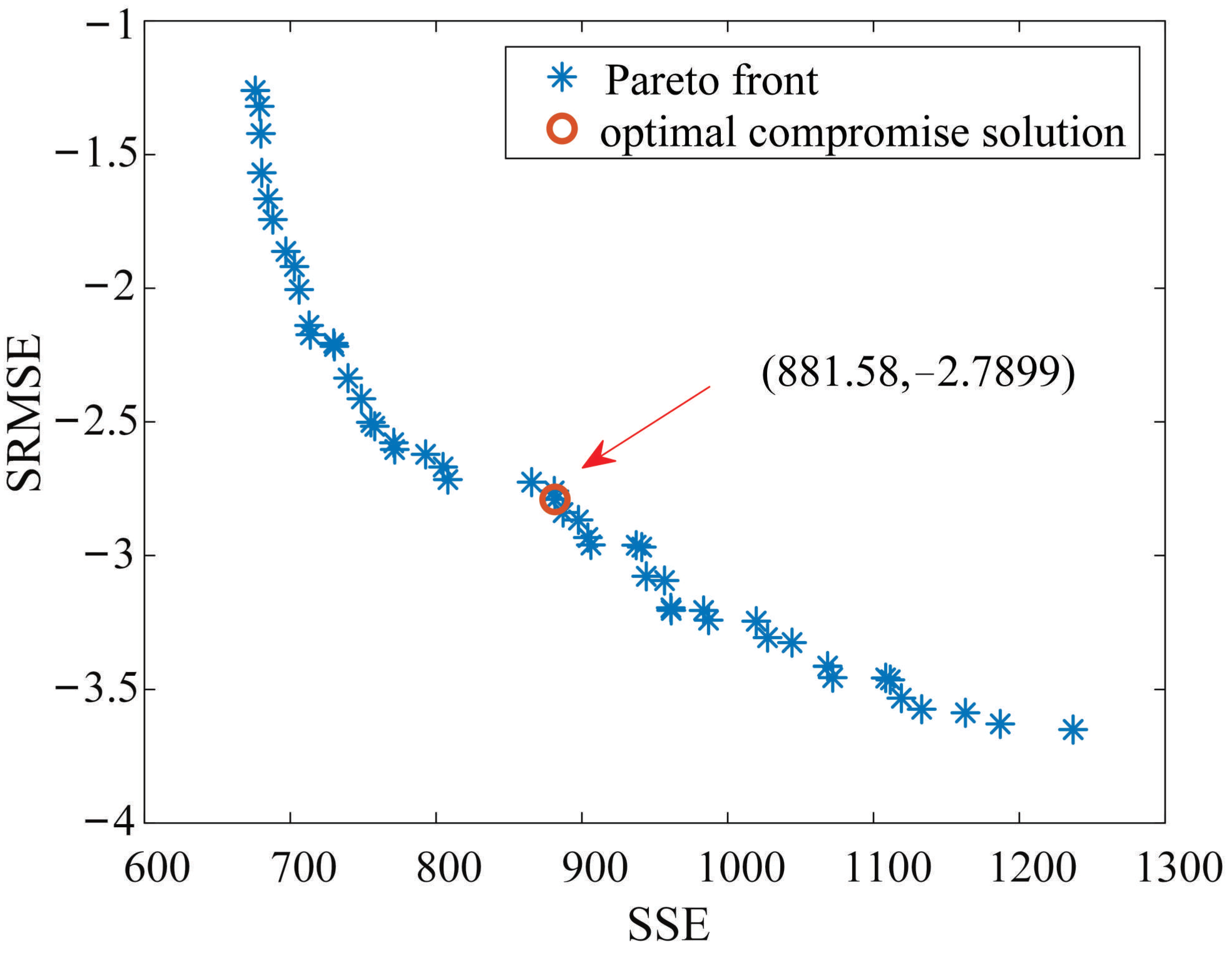
Figure 1. Idea of probability distribution modeling of multi-dimensional conditions for WPFE based on MNSGA-II-Kmeans.
Energies 15 02462 g001
Figure 2. PDF curves of WPFE and corresponding kurtosis.
Energies 15 02462 g002
Figure 3. The flowchart of MNSGA-II-Kmeans algorithm.
Energies 15 02462 g003
Figure 4. SSE-K curve obtained by elbow method.
Energies 15 02462 g004
Figure 5. SSE-K curves of each season.
Energies 15 02462 g005
Figure 6. Pareto front of season 1 of proposed multi-objective clustering model solved by MNSGA-II-Kmeans.
Energies 15 02462 g006
Figure 7. Clustering result of season 1.
Energies 15 02462 g007
Figure 8. PDF curves of each MDIF mode in season 1: (a) obtained by MNSGA-II-Kmeans; (b) obtained by Kmeans.
Energies 15 02462 g008
Figure 9. PDF curves of versatile distribution and actual distribution of WPFE in season 1, mode 1.
Energies 15 02462 g009
Figure 10. PDF curves of WPFE corresponding to mode 1 of season 1 in the initial training set and the initial testing set.
Energies 15 02462 g010
Figure 11. Experimental comparison of the SED problem: (a) using the non-conditional probability model of WPFE without considering the multi-dimensional conditional information; (b) using the proposed multi-dimensional conditional probability models of WPFE.
Energies 15 02462 g011
Table 1. Comparison of the clustering results of MNSGA-II-Kmeans and Kmeans.
SeasonMNSGA-II-KmeansKmeans
1NK78.02%57.78%
SRMSE2.78992.0424
SSE881.58805.83
2NK61.90%24.32%
SRMSE0.67150.4967
SSE1215.08999.08
3NK76.22%43.62%
SRMSE0.53960.5269
SSE1037.80890.99
4NK65.35%47.74%
SRMSE0.46170.4133
SSE852.44785.04
Table 2. Fitting and evaluation results of versatile distribution of WPFE.
MDIF Mode α β γ R 2 RMSE
Season 1Mode 119.921.267−0.03260.95960.2341
Mode 238.241.503−0.04490.97550.2680
Mode 37.6742.651−0.1490.99450.0564
Season 2Mode 115.851.559−0.06030.96370.2035
Mode 210.420.62780.10620.98540.0870
Season 3Mode 115.061.859−0.04770.96450.2834
Mode 211.680.58740.09640.98460.0906
Season 4Mode 110.521.562−0.04920.92890.2185
Mode 28.480.55280.09740.96970.1036
Table 3. SVM parameter optimization and verification results of each season.
Season C g Accuracy
(Optimized)
Accuracy
(Verified)
190.50970.176899.55%99.83%
21280.500099.72%99.89%
390.50970.353699.70%99.48%
4160.125099.81%99.59%
Table 4. Results of the proposed SED problem.
Probability Model of WPFE UsedSystem Wind Power Consumption
(MWh)
LLCR
Non-conditional22,370.2398.50%
Proposed multi-dimensional conditional23,765.1596.09%
Publisher’s Note: MDPI stays neutral with regard to jurisdictional claims in published maps and institutional affiliations.

