Author Contributions
Conceptualization, A.F. and T.A.G.; methodology, A.F. and T.A.G.; software, A.F. and T.A.G.; validation, A.F. and T.A.G.; formal analysis, A.F. and T.A.G.; investigation, A.F. and T.A.G.; resources, A.F. and T.A.G.; data curation, A.F. and T.A.G.; writing—original draft preparation, A.F. and T.A.G.; writing—review and editing, A.F., T.A.G., D.M., P.G.A. and G.P.; visualization, A.F. and T.A.G.; supervision, D.M., P.G.A. and G.P.; project administration, D.M. and G.P.; All authors have read and agreed to the published version of the manuscript.
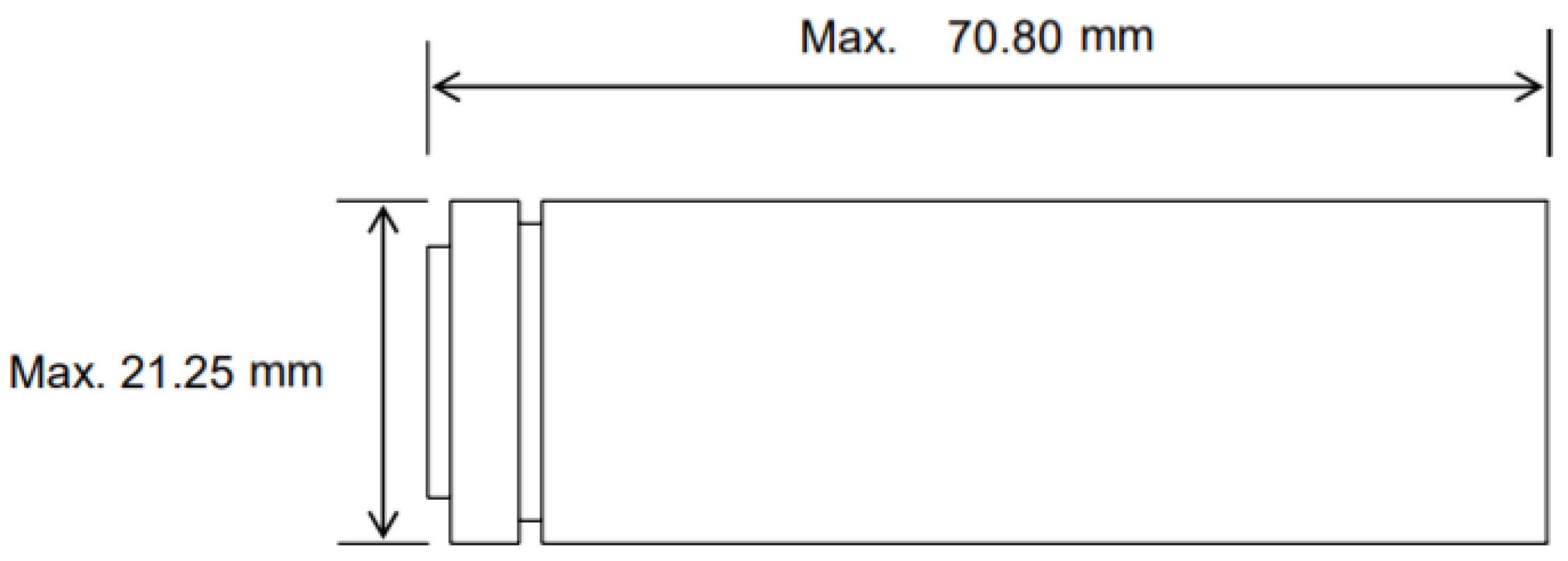
Figure 1.
Outline dimensions of INR21700-50E.
Figure 1.
Outline dimensions of INR21700-50E.
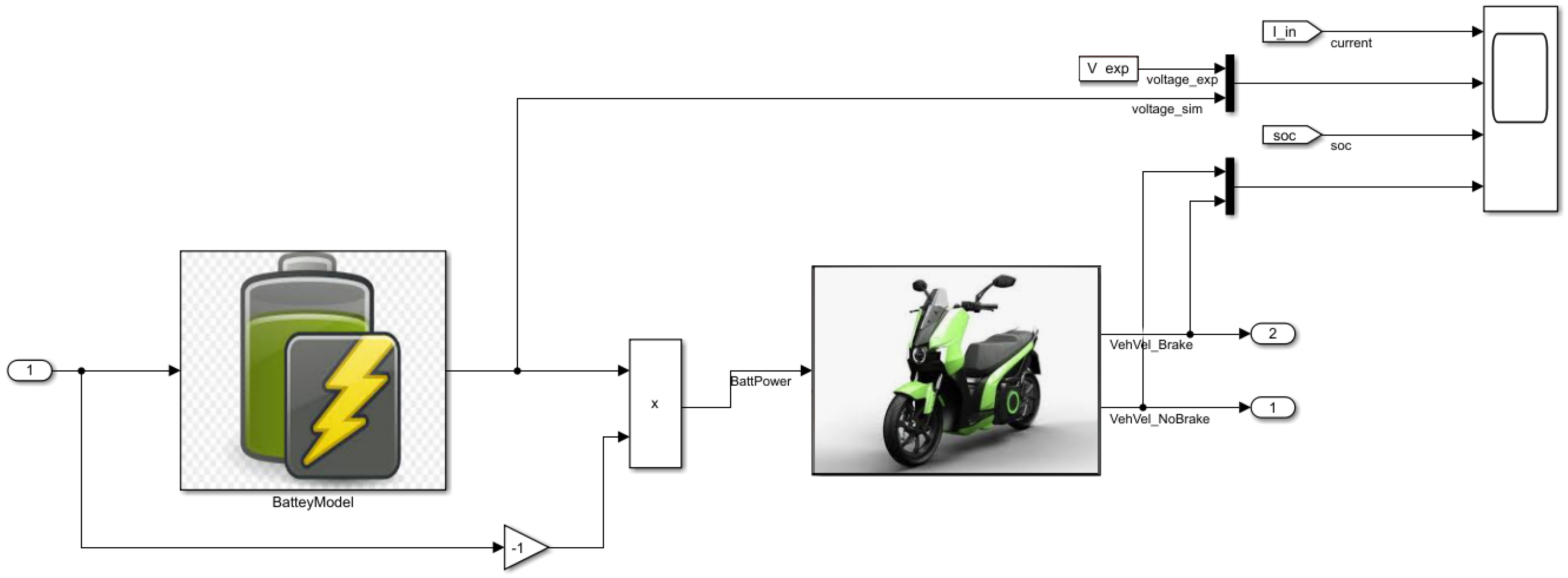
Figure 2.
Global model implemented on Simulink. It includes the battery model connected to the the dynamic vehicle model.
Figure 2.
Global model implemented on Simulink. It includes the battery model connected to the the dynamic vehicle model.
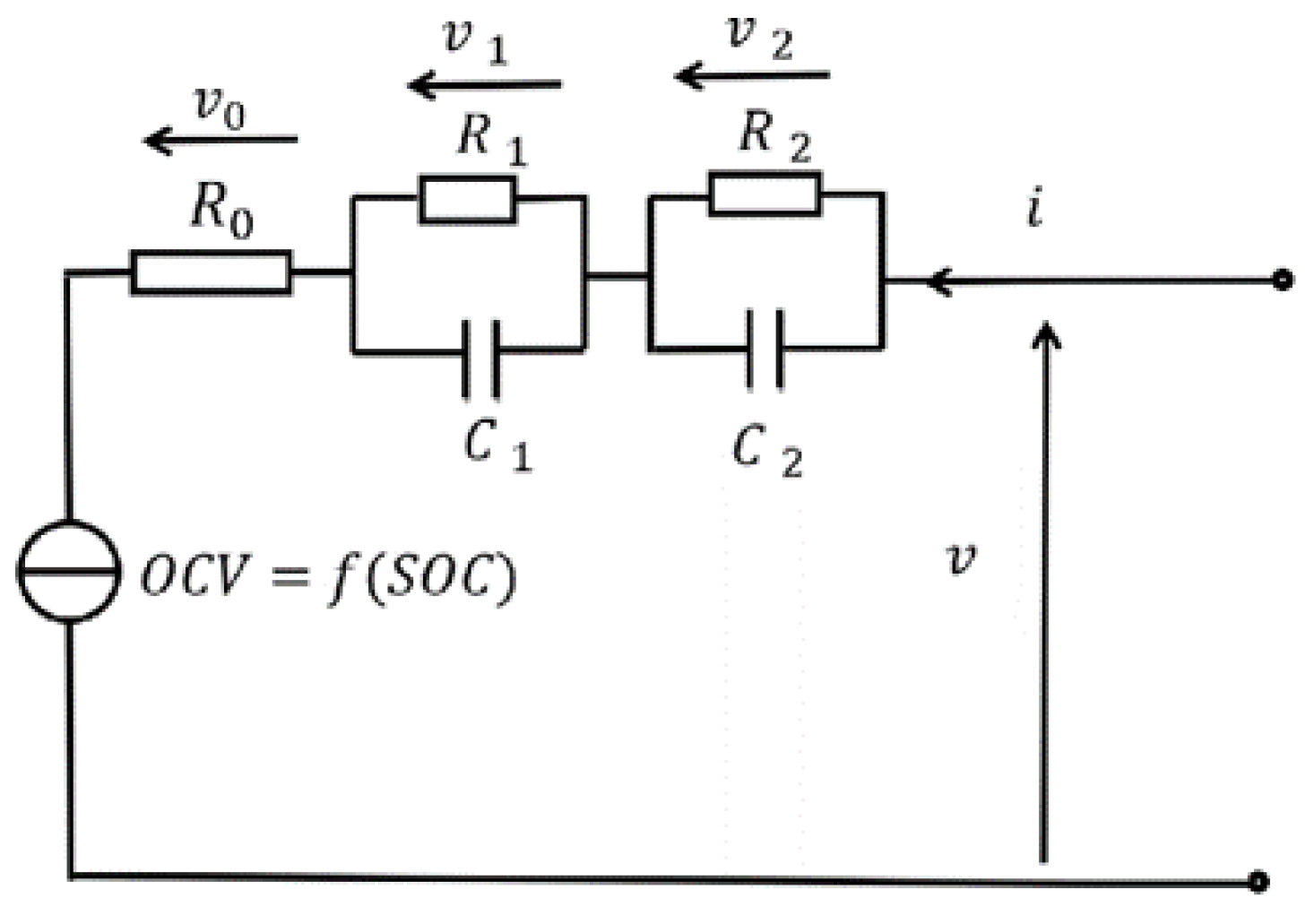
Figure 3.
The Equivalent Circuit Model of lithium-ion battery with all model parameters which describe the operation of a single cell.
Figure 3.
The Equivalent Circuit Model of lithium-ion battery with all model parameters which describe the operation of a single cell.
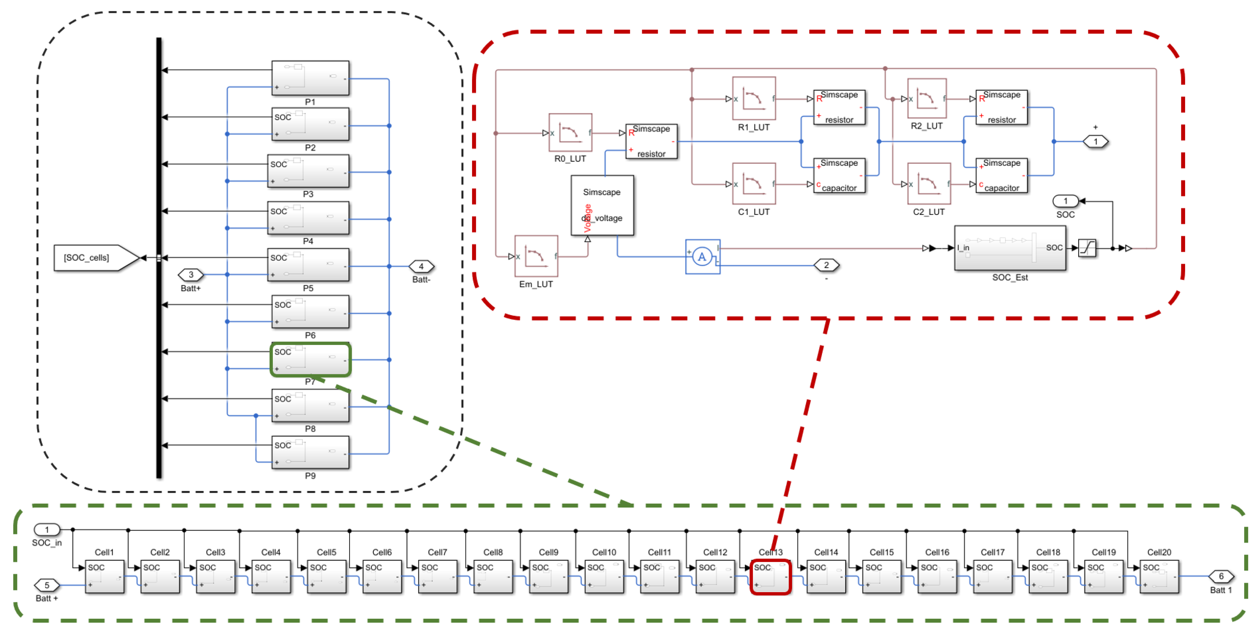
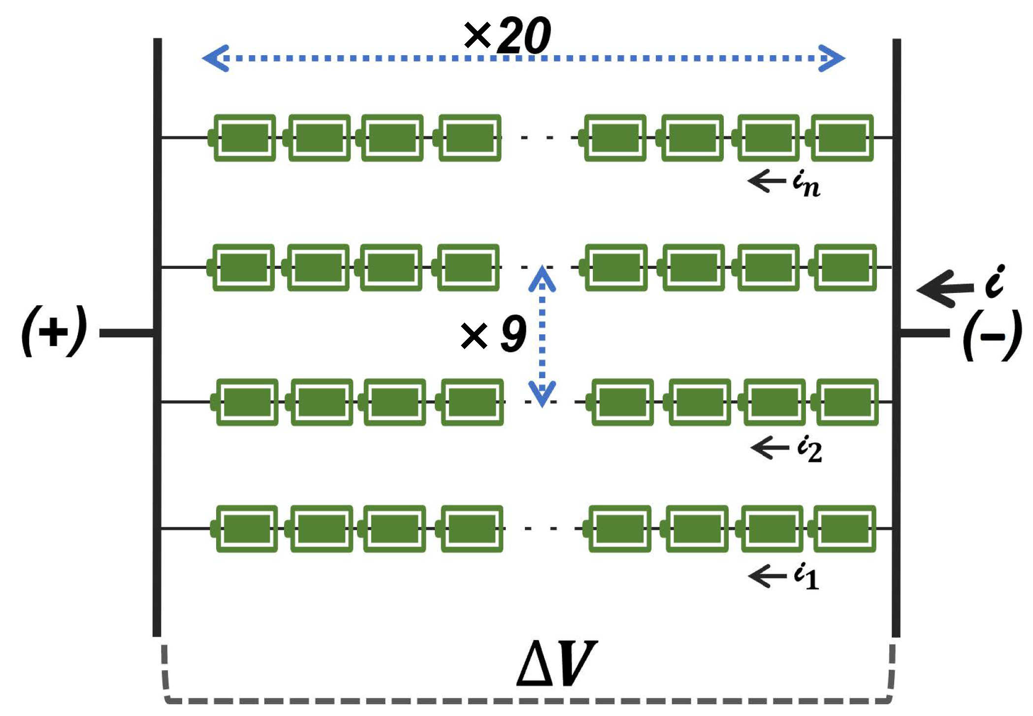
Figure 4.
Battery pack modeling: 9 modules are connected in parallel and each module has 20 cells connected in series, each single one modeled as an independent ECM: ’i’ is the battery pack current, and is the voltage of the battery pack.
Figure 4.
Battery pack modeling: 9 modules are connected in parallel and each module has 20 cells connected in series, each single one modeled as an independent ECM: ’i’ is the battery pack current, and is the voltage of the battery pack.
Figure 5.
Model of the battery pack configuration on Simulink virtual environment.
Figure 5.
Model of the battery pack configuration on Simulink virtual environment.
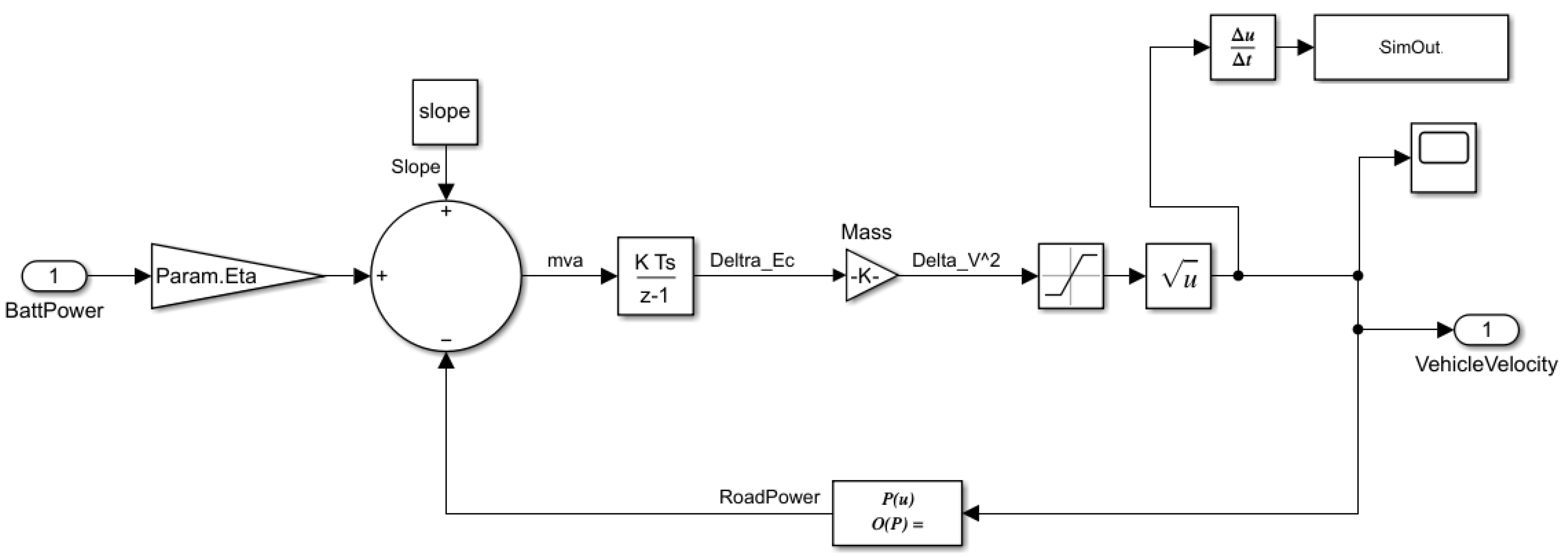
Figure 6.
Longitudinal dynamics of two-wheeler block using through a physical-based energy approach on Simulink.
Figure 6.
Longitudinal dynamics of two-wheeler block using through a physical-based energy approach on Simulink.
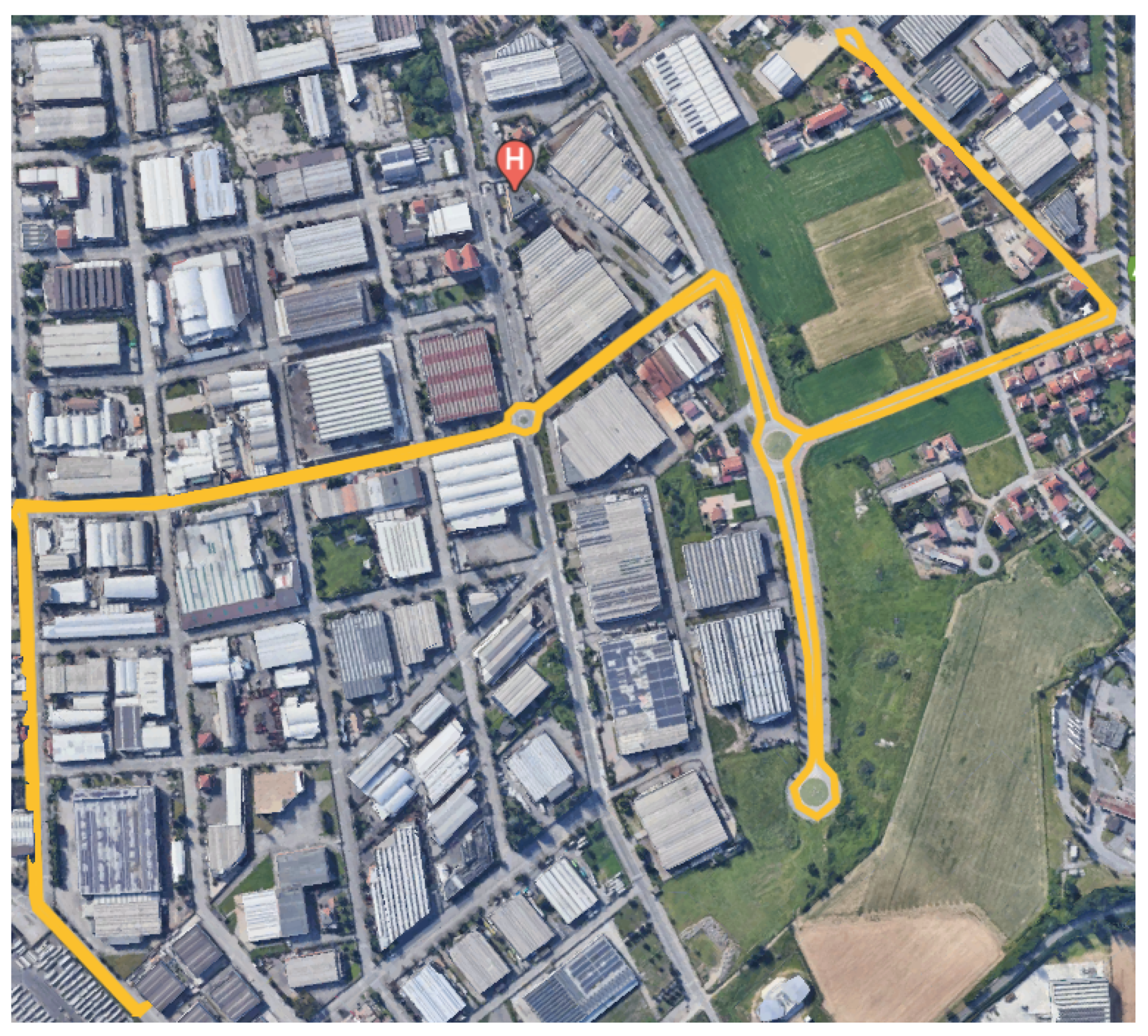
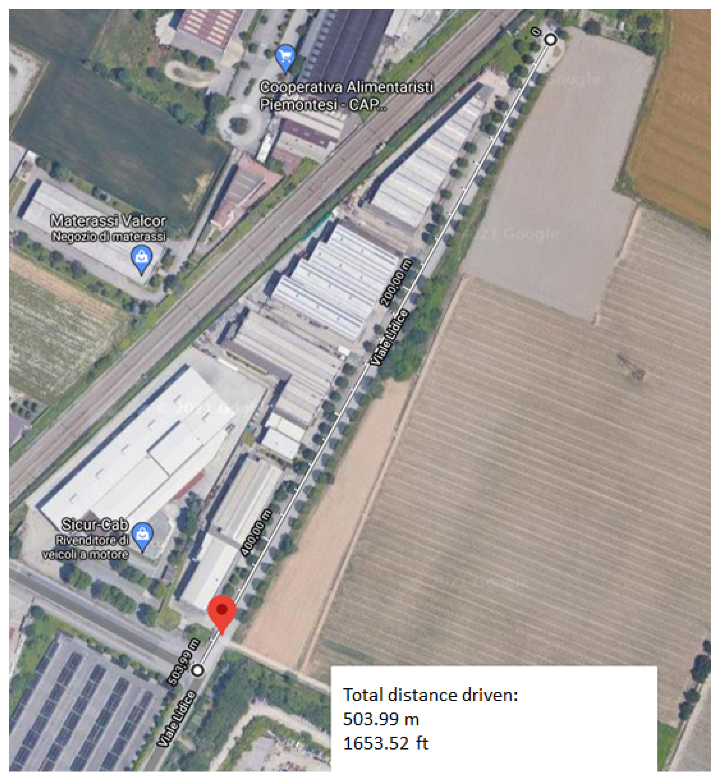
Figure 7.
Selected route in Turin, Italy, for performing on-road tests for the prototype two-wheeler. The route is driven to calibrate the battery model.
Figure 7.
Selected route in Turin, Italy, for performing on-road tests for the prototype two-wheeler. The route is driven to calibrate the battery model.
Figure 8.
Selected route in Turin, Italy, forperforming on-road tests for the prototype two-wheeler. The route is driven to calibrate the dynamic vehicle model.
Figure 8.
Selected route in Turin, Italy, forperforming on-road tests for the prototype two-wheeler. The route is driven to calibrate the dynamic vehicle model.
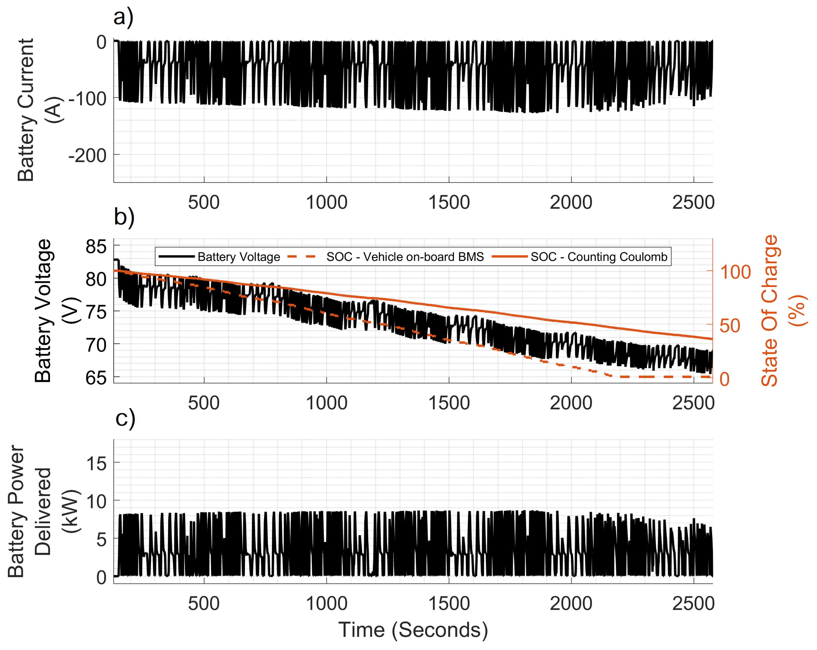
Figure 9.
Test #1: (a) current (b) voltage and (c) power delivered by the battery during a drive mission for a discharging test session with the SOC estimation performed by the stock BMS of the electrical vehicle and by a post-processing of the data through the Counting Coulomb method.
Figure 9.
Test #1: (a) current (b) voltage and (c) power delivered by the battery during a drive mission for a discharging test session with the SOC estimation performed by the stock BMS of the electrical vehicle and by a post-processing of the data through the Counting Coulomb method.
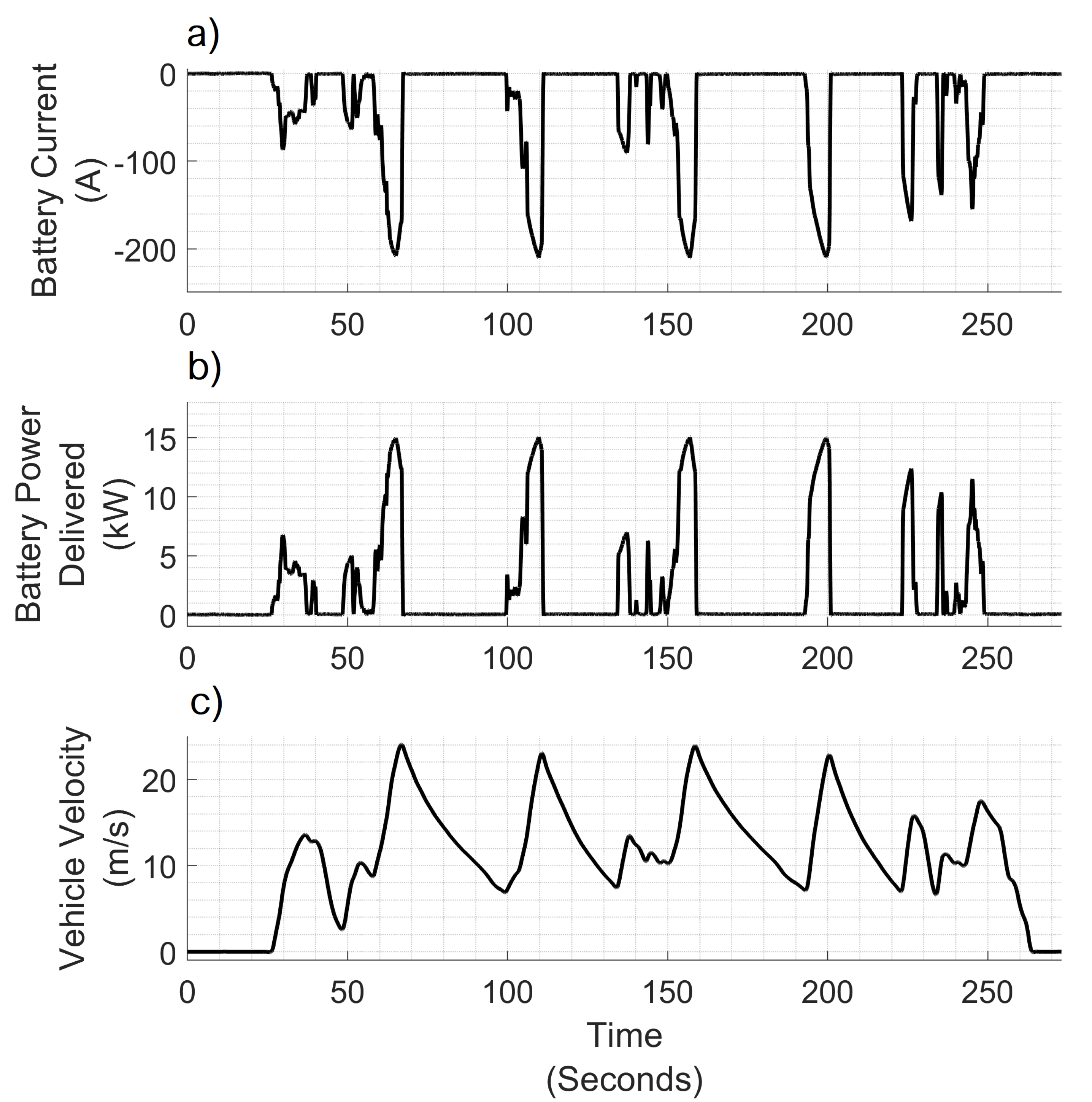
Figure 10.
Test #3.1: (a) current and (b) power (kW) delivered from the battery and (c) vehicle velocity profile during a Coastdown test session composed by several acceleration and deceleration phases.
Figure 10.
Test #3.1: (a) current and (b) power (kW) delivered from the battery and (c) vehicle velocity profile during a Coastdown test session composed by several acceleration and deceleration phases.
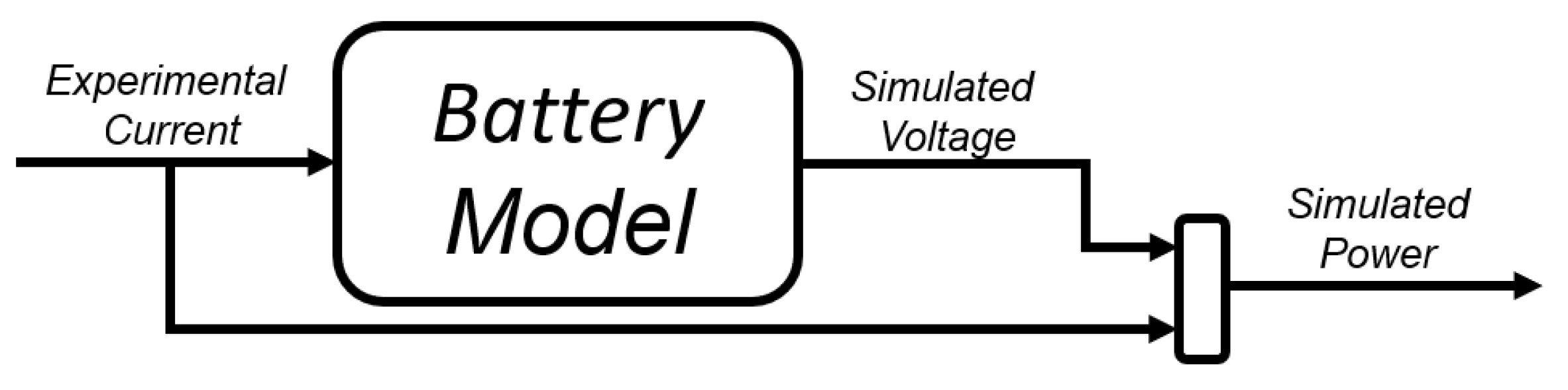
Figure 11.
Battery model I/O scheme.
Figure 11.
Battery model I/O scheme.
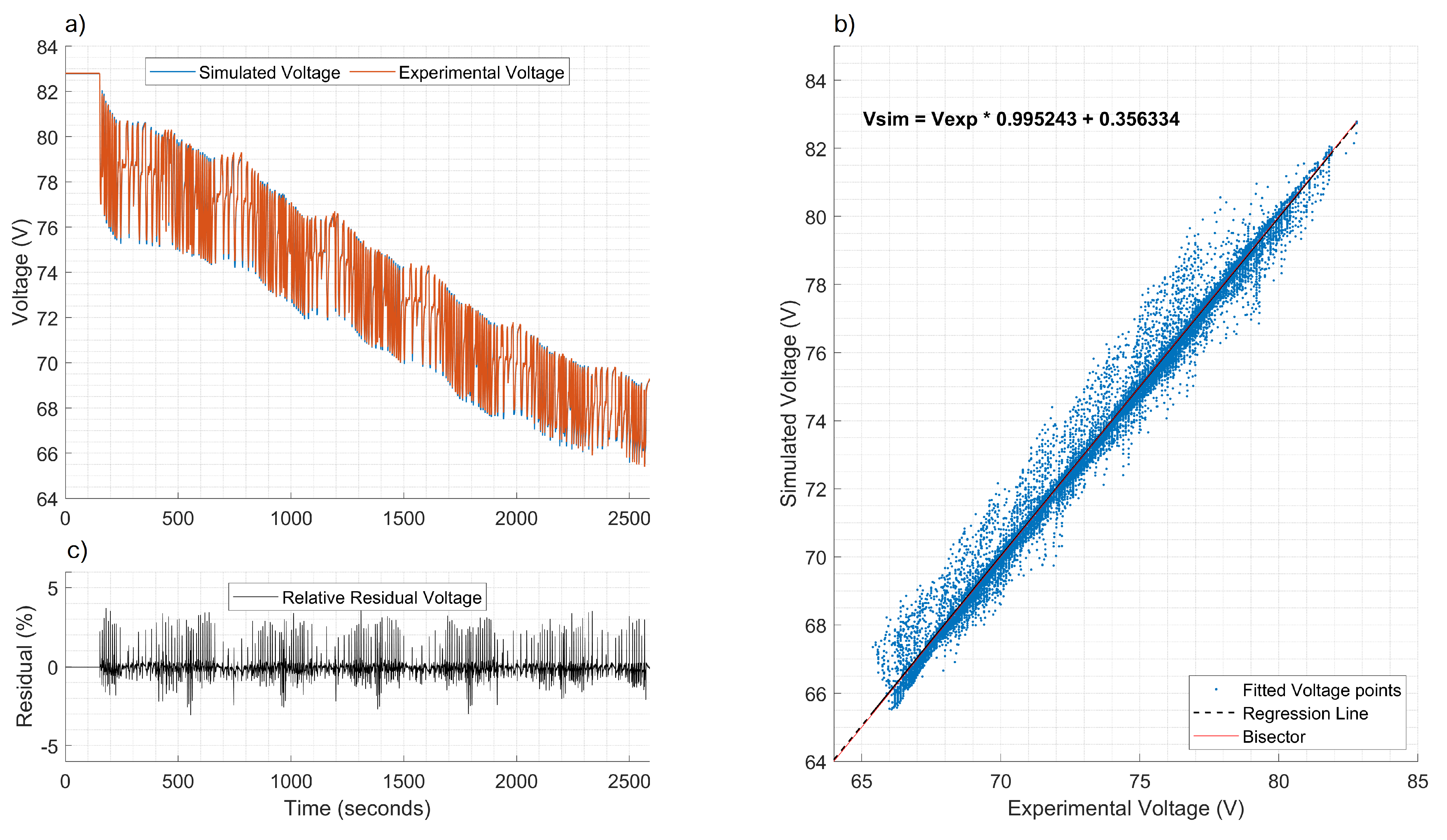
Figure 12.
Test #1.1: regression process results for estimation of model voltage. (a) The simulated voltage and experimental voltage on real driving mission and (c) residual error of estimation. (b) Regression process results in terms of fitting equation and bisector comparison.
Figure 12.
Test #1.1: regression process results for estimation of model voltage. (a) The simulated voltage and experimental voltage on real driving mission and (c) residual error of estimation. (b) Regression process results in terms of fitting equation and bisector comparison.
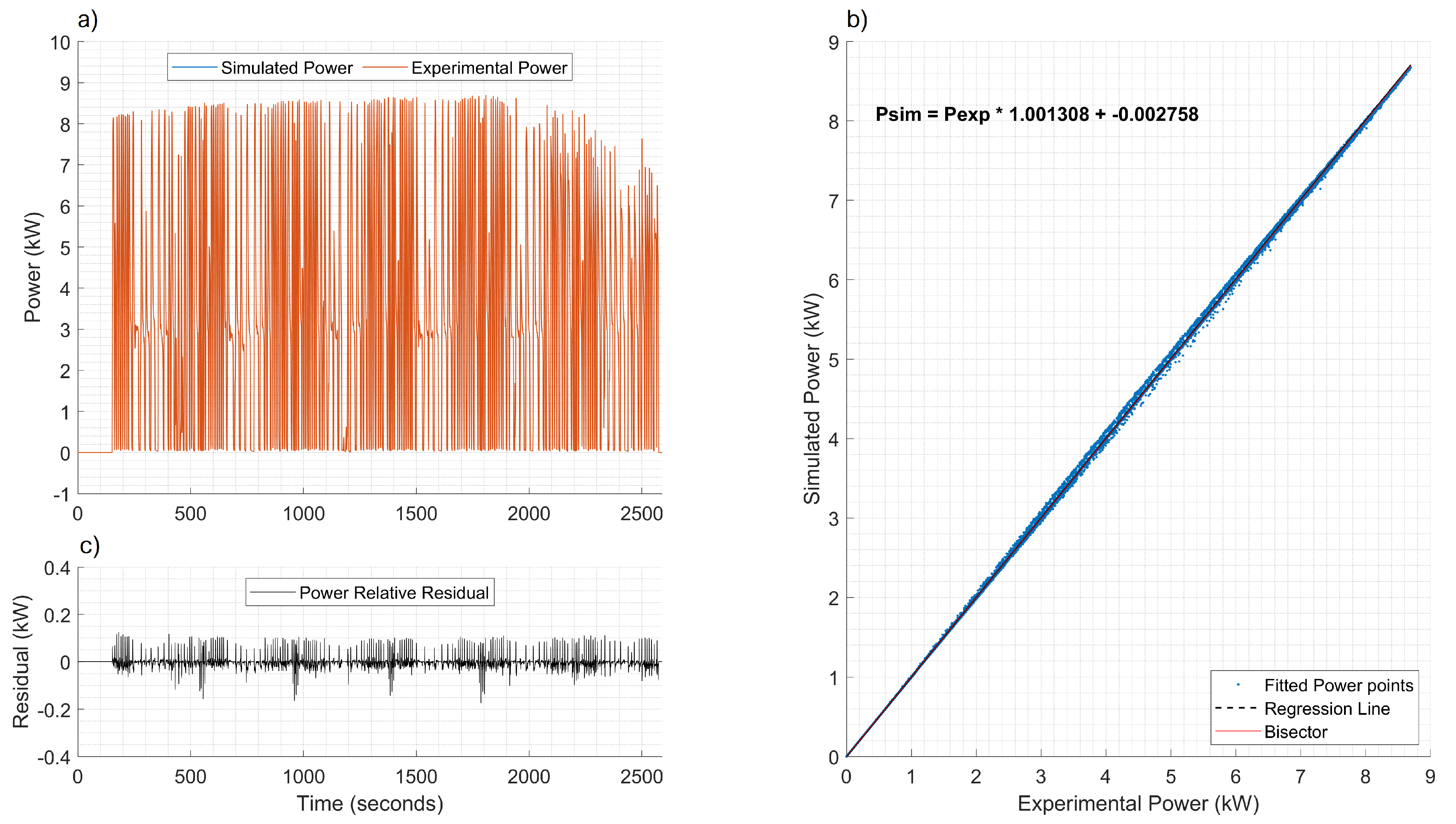
Figure 13.
Test #1.1: Regression process results for estimation of model power. (a) The simulated and experimental power on real driving mission and (c) residual error of estimation. (b) Regression process results in terms of fitting equation and bisector comparison.
Figure 13.
Test #1.1: Regression process results for estimation of model power. (a) The simulated and experimental power on real driving mission and (c) residual error of estimation. (b) Regression process results in terms of fitting equation and bisector comparison.
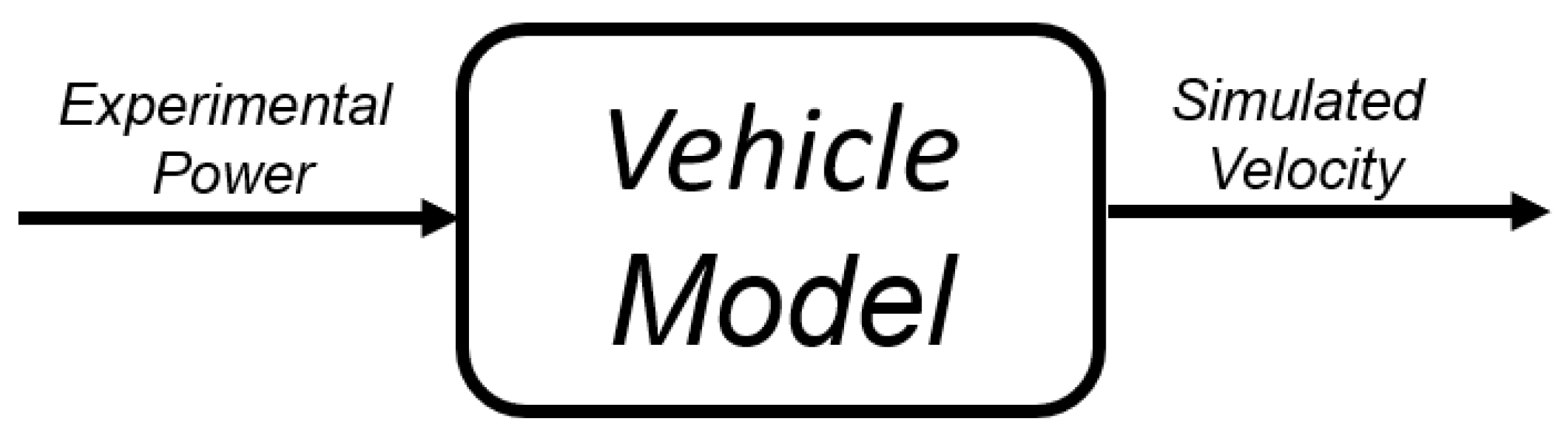
Figure 14.
Vehicle model input/output scheme.
Figure 14.
Vehicle model input/output scheme.
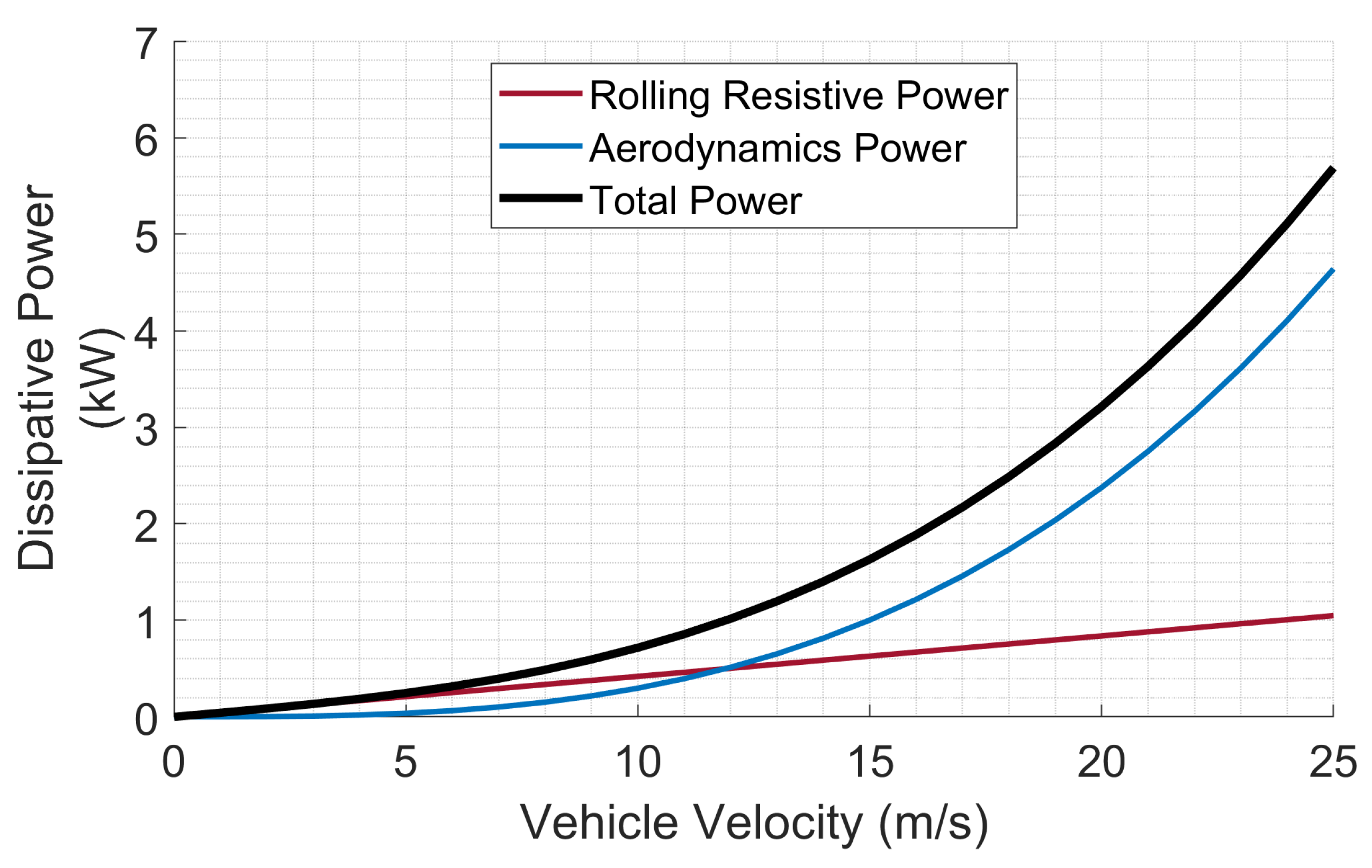
Figure 15.
Road load power terms acting on vehicle body as a velocity-dependent function.
Figure 15.
Road load power terms acting on vehicle body as a velocity-dependent function.
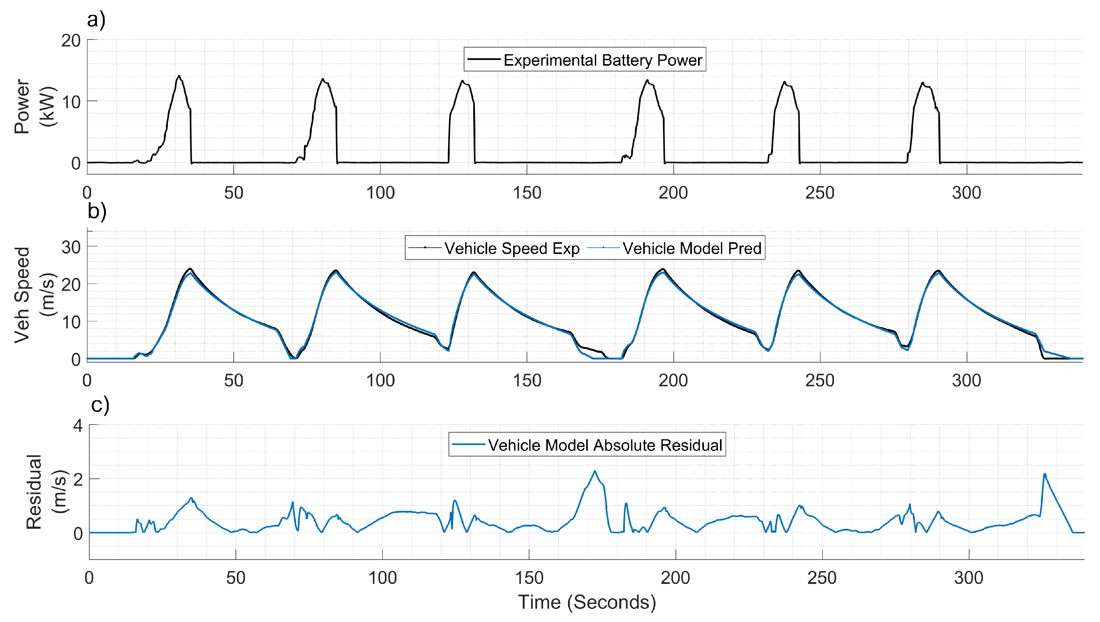
Figure 16.
Test #4.1. Vehicle model performance: (a) battery power delivered, (b) predicted and measured velocity and (c) residual of the estimation.
Figure 16.
Test #4.1. Vehicle model performance: (a) battery power delivered, (b) predicted and measured velocity and (c) residual of the estimation.
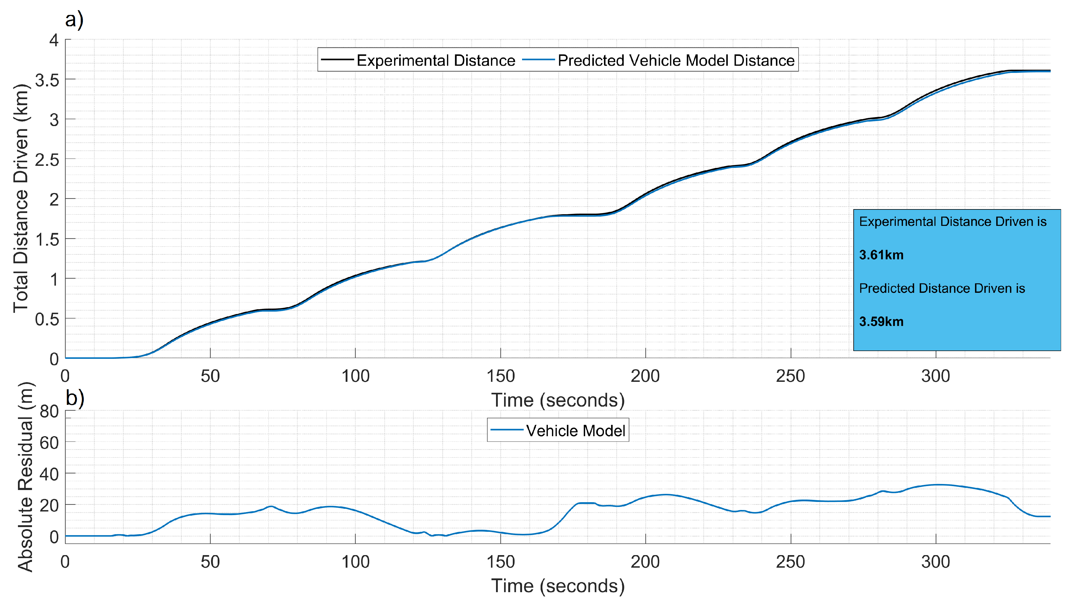
Figure 17.
Test #4.1. Electric range prediction: (a) total distance traveled and (b) instantaneous absolute residual.
Figure 17.
Test #4.1. Electric range prediction: (a) total distance traveled and (b) instantaneous absolute residual.
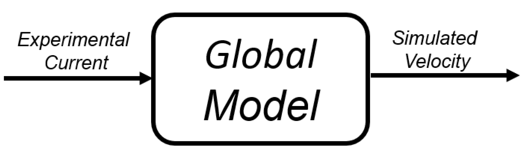
Figure 18.
Global model I/O scheme.
Figure 18.
Global model I/O scheme.
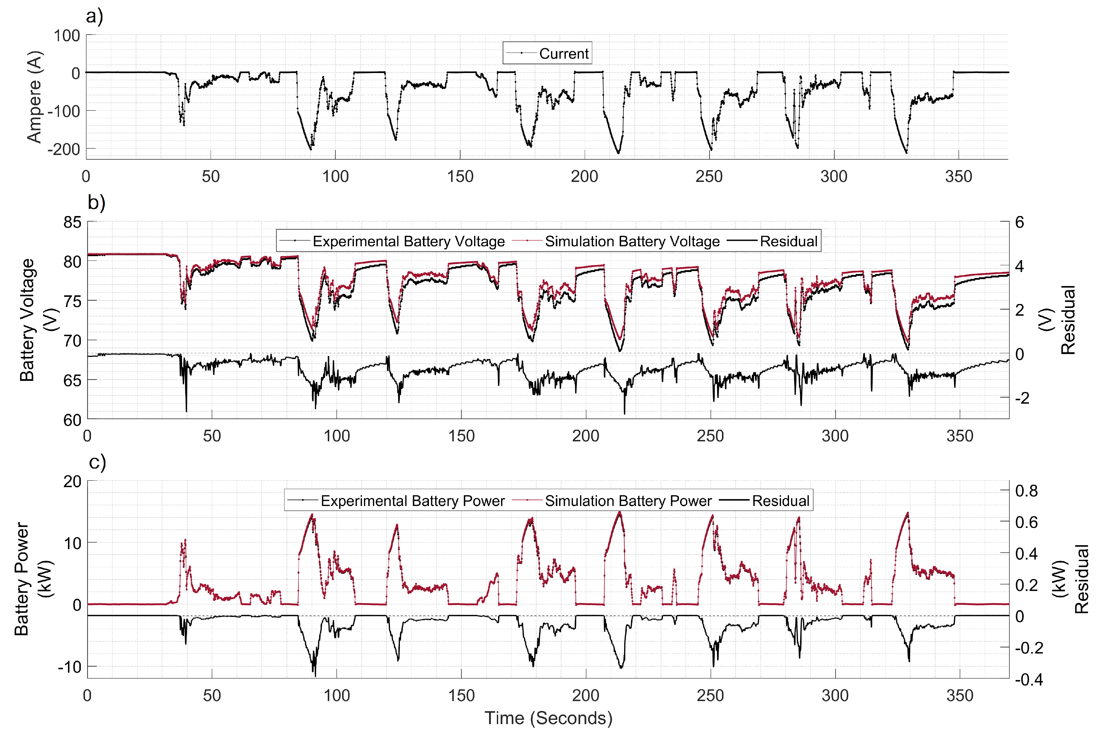
Figure 19.
Test #6.4: (a) battery pack electrical current (A) as global model input, (b) battery pack voltage and (c) total battery pack power.
Figure 19.
Test #6.4: (a) battery pack electrical current (A) as global model input, (b) battery pack voltage and (c) total battery pack power.
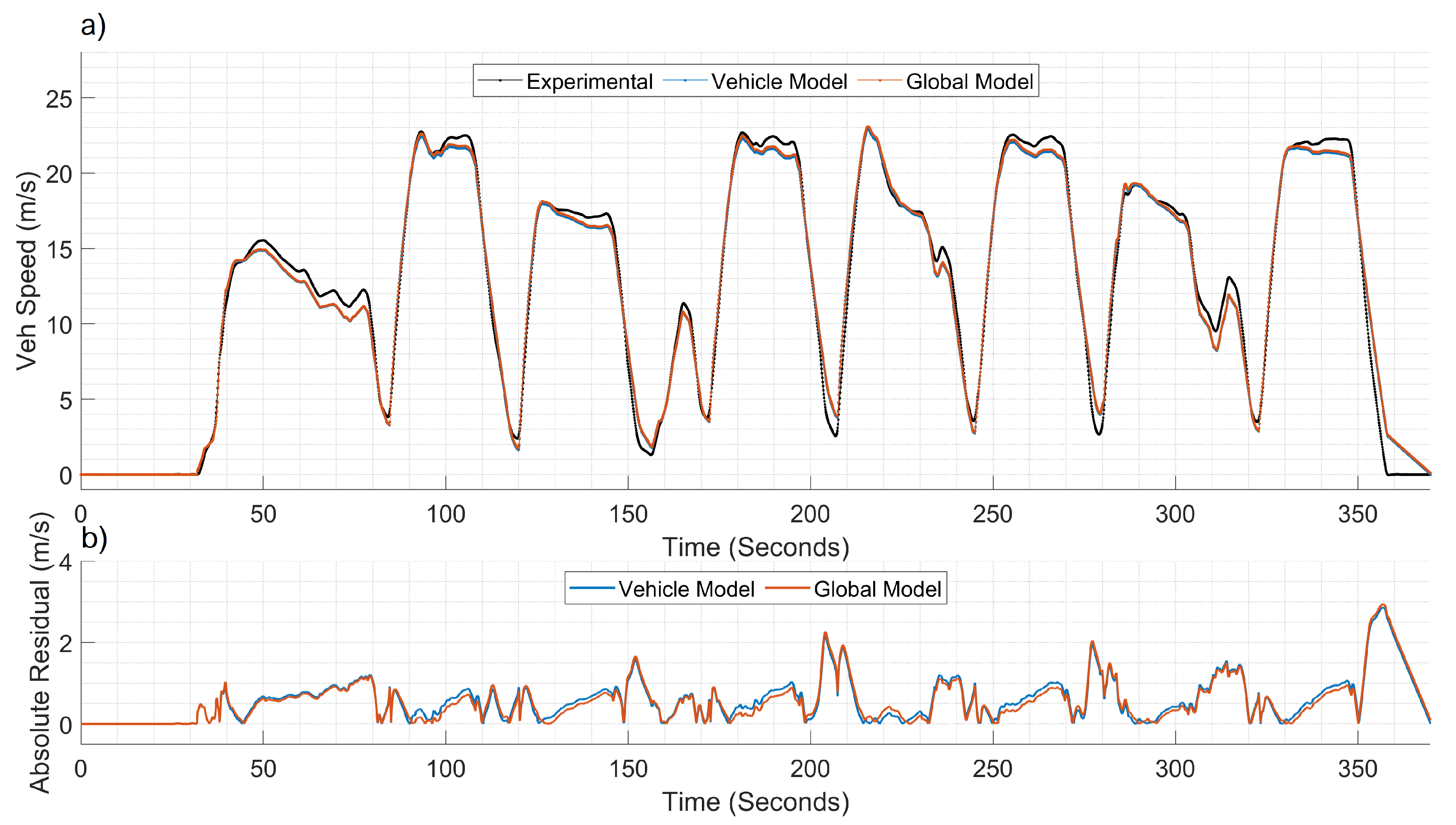
Figure 20.
Test #6.4. Two-wheeler performance prediction: (a) the vehicle speed (m/s) of the global model compared to that of the single vehicle model and experimental data, (b) absolute residual error of global and vehicle models.
Figure 20.
Test #6.4. Two-wheeler performance prediction: (a) the vehicle speed (m/s) of the global model compared to that of the single vehicle model and experimental data, (b) absolute residual error of global and vehicle models.
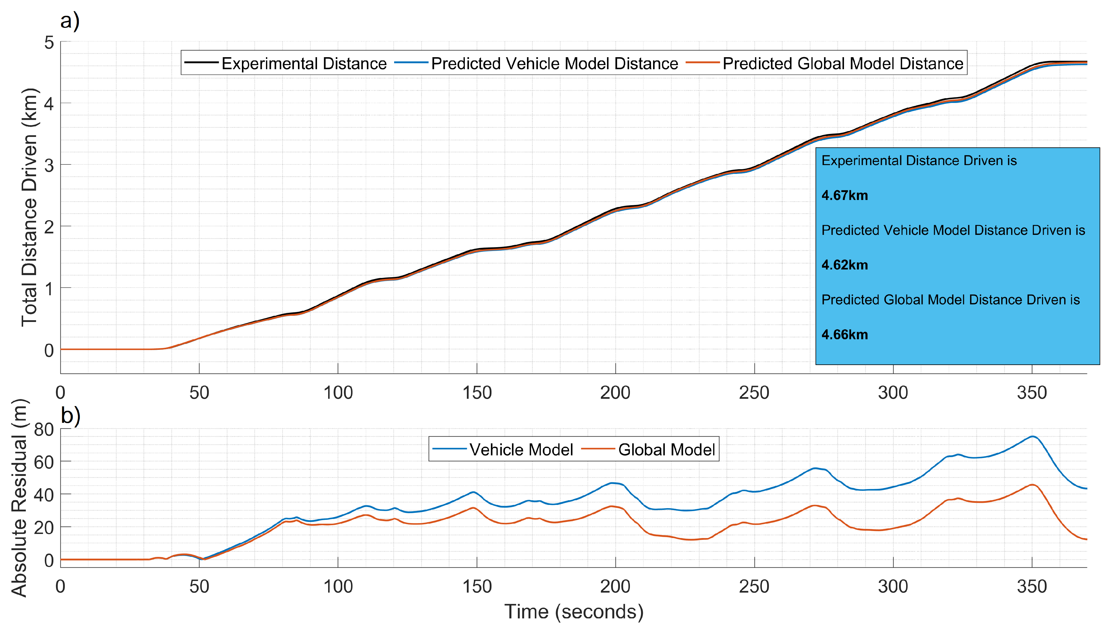
Figure 21.
Test #6.4. (a) Total distance traveled by the two-wheeler expressed as electric range is estimated by the global model and compared with that of single vehicle model and experimental data. (b) Absolute residual error is plotted over the test time.
Figure 21.
Test #6.4. (a) Total distance traveled by the two-wheeler expressed as electric range is estimated by the global model and compared with that of single vehicle model and experimental data. (b) Absolute residual error is plotted over the test time.
Table 1.
Technical specifications of SAMSUNG INR21700-50E cell as reported on Samsung company datasheet [
20].
Table 1.
Technical specifications of SAMSUNG INR21700-50E cell as reported on Samsung company datasheet [
20].
| Parameters | Values | Measurement Unit |
|---|
| Cell Format | Cylindrical | - |
| Technology | Li-Ion | - |
| Nominal Voltage | 3.6 | V |
| Nominal Capacity | 4.9 | Ah |
| Maximum continuous discharge current | 9.8 | A |
| Maximum non continuous discharge current | 14.7 | A |
| Recharge maximum current | 4.9 | A |
| Discharge Cut-off Voltage | 2.5 | V |
Table 2.
Technical specification of the prototype battery pack.
Table 2.
Technical specification of the prototype battery pack.
| Parameters | Values | Measurement Unit |
|---|
| Pack configuration | 20s9p | - |
| Nominal Voltage | 72 | V |
| Nominal Capacity | 44.1 | Ah |
| Total Energy | 3.17 | kWh |
| Maximum continuous discharge current | 88.2 | A |
| Maximum non continuous discharge current | 117.6 | A |
| weight | 12.5 | kg |
Table 3.
Test Session dataset available for the model identification.
Table 3.
Test Session dataset available for the model identification.
| Test | Test Type/Session | Test Specifications | Repetitions |
|---|
| 1 | Discharge | SOC in range [1, 0.3] | 1 |
| 2.1 | Coastdown 1 | (from 22 to 8) m/s | 4 |
| 3.1 | Coastdown 2 | (from 22 to 8) m/s | 4 |
| 3.2 | Coastdown 2 | (from 22 to 8) m/s | 4 |
| 4.1 | Coastdown 3 | (from 22 to 8) m/s | 4 |
| 4.2 | Coastdown 3 | (from 22 to 8) m/s | 4 |
| 5.1 | Constant Speed 1 | 5.5 m/s | 2 |
| 5.2 | Constant Speed 1 | 11 m/s | 2 |
| 5.3 | Constant Speed 1 | 16.5 m/s | 2 |
| 5.4 | Constant Speed 1 | 22 m/s | 2 |
| 6.1 | Constant Speed 2 | 5.5 m/s | 2 |
| 6.2 | Constant Speed 2 | 11 m/s | 2 |
| 6.3 | Constant Speed 2 | 16.5 m/s | 2 |
| 6.4 | Constant Speed 2 | 22 m/s | 2 |
| 7 | Partial Knob | 50% | 1 |
Table 4.
Used Datasets for model identification and testing, with reference to
Table 3.
Table 4.
Used Datasets for model identification and testing, with reference to
Table 3.
| | Model Identification | Model Testing |
|---|
| Battery Model | 1 | 3.2–4.2–6–7 |
| Dynamic Vehicle Model | 2.1–3.1–4.1–5 | 3.2–4.2–6–7 |
| Global Model | - | 3.2–4.2–6–7 |
Table 5.
Battery Parameter Identification Voltage Metrics.
Table 5.
Battery Parameter Identification Voltage Metrics.
| Test # | RMSE (V) | |
|---|
| 1 | 0.383 | 0.993 |
Table 6.
Battery Parameter Identification Power and Energy Metrics.
Table 6.
Battery Parameter Identification Power and Energy Metrics.
| Test # | RMSE (kW) | | Experimental Energy Delivered (Wh) | Simulation Energy Delivered (Wh) | Relative Error Energy (%) |
|---|
| 1 | 0.022 | 0.999 | 2409.3 | 2407.9 | 0.058 |
Table 7.
Battery Testing Voltage Metrics.
Table 7.
Battery Testing Voltage Metrics.
| Test # | RMSE (V) | |
|---|
| 3.2 | 0.344 | 0.984 |
| 4.2 | 0.75 | 0.983 |
| 6.1 | 0.393 | 0.960 |
| 6.2 | 0.568 | 0.989 |
| 6.3 | 0.727 | 0.984 |
| 6.4 | 0.815 | 0.987 |
| 7 | 0.181 | 0.981 |
Table 8.
Battery Testing Power and Energy Metrics.
Table 8.
Battery Testing Power and Energy Metrics.
| Test # | RMSE (kW) | | Experimental Energy Delivered (Wh) | Simulation Energy Delivered (Wh) | Error Energy (%) |
|---|
| 3.2 | 0.035 | 0.999 | 158.8 | 157.9 | 0.527 |
| 4.2 | 0.076 | 0.999 | 158.6 | 161.5 | 1.852 |
| 6.1 | 0.006 | 0.999 | 54.5 | 54.9 | 0.573 |
| 6.2 | 0.022 | 0.999 | 114.8 | 115.9 | 0.980 |
| 6.3 | 0.051 | 0.999 | 190.7 | 193.2 | 1.300 |
| 6.4 | 0.079 | 0.999 | 308.7 | 312.9 | 1.382 |
| 7 | 0.007 | 0.999 | 86.3 | 86.5 | 0.182 |
Table 9.
Coastdown coefficients values for longitudinal dynamic vehicle modeling. A, B and C are the coefficients for describing the resistive forces depending on the vehicle speed.
Table 9.
Coastdown coefficients values for longitudinal dynamic vehicle modeling. A, B and C are the coefficients for describing the resistive forces depending on the vehicle speed.
| Parameter | Value | U.d.m. |
|---|
| A | 41.8 | N |
| B | 0 | |
| C | 0.3 | |
Table 10.
Vehicle dynamic model coefficients: m is the sum of the vehicle and driver masses, is the value of the equivalent inertia of the rotating components and is the overall battery-to-road efficiency, including the electric motors and transmission losses.
Table 10.
Vehicle dynamic model coefficients: m is the sum of the vehicle and driver masses, is the value of the equivalent inertia of the rotating components and is the overall battery-to-road efficiency, including the electric motors and transmission losses.
| Name | Value | U.d.m. |
|---|
| m | 184 | kg |
| 16 | kg |
| 0.75 | - |
Table 11.
Aerodynamic and rolling resistance coefficient values of two-wheeler road load model.
Table 11.
Aerodynamic and rolling resistance coefficient values of two-wheeler road load model.
| Aerodynamic drag coefficient | | 0.81 | - |
| Rolling resistance coefficient | f | 11.62 | |
Table 12.
Prediction metrics of vehicle model performance over parameter identification datasets.
Table 12.
Prediction metrics of vehicle model performance over parameter identification datasets.
| Test # | RMSE (m/s) | | Total Distance Traveled Experimental (km) | Total Distance Traveled Model (km) | Error Distance (%) |
|---|
| 2.1 | 0.631 | 0.990 | 4.100 | 4.035 | 1.578 |
| 3.1 | 0.750 | 0.986 | 3.006 | 3.014 | 0.272 |
| 4.1 | 0.577 | 0.994 | 3.607 | 3.594 | 0.346 |
| 5.1 | 0.846 | 0.933 | 1.200 | 1.021 | 15.009 |
| 5.2 | 0.923 | 0.984 | 1.334 | 1.210 | 9.272 |
| 5.3 | 0.942 | 0.976 | 3.730 | 3.607 | 3.294 |
| 5.4 | 1.13 | 0.977 | 4.236 | 4.252 | 0.381 |
Table 13.
Prediction metrics of vehicle model performance over testing datasets.
Table 13.
Prediction metrics of vehicle model performance over testing datasets.
| Test # | RMSE (m/s) | | Total Distance Traveled Experimental (km) | Total Distance Traveled Model (km) | Error Distance (%) |
|---|
| 3.2 | 0.914 | 0.978 | 3.13 | 3.12 | 0.496 |
| 4.2 | 0.503 | 0.996 | 3.60 | 3.61 | 0.334 |
| 6.1 | 0.507 | 0.974 | 1.95 | 1.86 | 4.90 |
| 6.2 | 0.638 | 0.987 | 2.98 | 2.85 | 4.41 |
| 6.3 | 0.908 | 0.982 | 3.48 | 3.42 | 1.89 |
| 6.4 | 0.788 | 0.991 | 4.67 | 4.62 | 0.93 |
| 7 | 1.171 | 0.973 | 1.59 | 1.53 | 3.32 |
Table 14.
Prediction metrics of global model performance over testing datasets.
Table 14.
Prediction metrics of global model performance over testing datasets.
| Test # | RMSE (m/s) | | Total Distance Traveled Experimental (km) | Total Distance Traveled Model (km) | Error Distance (%) |
|---|
| 3.2 | 0.917 | 0.978 | 3.13 | 3.11 | 0.763 |
| 4.2 | 0.503 | 0.996 | 3.60 | 3.64 | 1.106 |
| 6.1 | 0.492 | 0.975 | 1.95 | 1.87 | 4.539 |
| 6.2 | 0.610 | 0.987 | 2.98 | 2.87 | 3.855 |
| 6.3 | 0.892 | 0.982 | 3.48 | 3.44 | 1.209 |
| 6.4 | 0.777 | 0.991 | 4.67 | 4.66 | 0.263 |
| 7 | 1.169 | 0.973 | 1.59 | 1.53 | 3.225 |


 ,
, 


