Abstract
Dynamic programming (DP) is currently the reference optimal energy management approach for hybrid electric vehicles (HEVs). However, several research concerns arise regarding the effective application of DP for optimal HEV control problems which involve a significant number of control variables, state variables and optimization constraints. This paper deals with an optimal control problem for a full parallel P2 HEV with constraints on battery state-of-charge (SOC), battery lifetime in terms of state-of-health (SOH), and smooth driving in terms of the frequencies of internal combustion engine (ICE) activations and gear shifts over time. The DP formulation for the considered HEV control problem is outlined, yet its practical application is demonstrated as unfeasible due to a lack of computational power and memory in current desktop computers. To overcome this drawback, a computationally efficient version of DP is proposed which is named Slope-weighted Rapid Dynamic Programming (SRDP). Computational advantage is achieved by SRDP in considering only the most efficient HEV powertrain operating points rather than the full set of control variable values at each time instant of the drive cycle. A benchmark study simulating various drive cycles demonstrates that the introduced SRDP can achieve compliance with imposed control constraints on battery SOC, battery SOH and smooth driving. At the same time, SRDP can achieve up to 78% computational time saving compared with a baseline DP approach considering the Worldwide Harmonized Light Vehicle Test Procedure (WLTP). On the other hand, the increase in the fuel consumption estimated by SRDP is limited within 3.3% compared with the baseline DP approach if the US06 Supplemental Federal Test Procedure is considered. SRDP could thus be exploited to efficiently explore the large design space associated to HEV powertrains.
1. Introduction
Hybrid electric vehicles (HEVs) are a fundamental technology to reduce the fuel consumption and pollutant emissions of road vehicles [1,2,3]. Nevertheless, a remarkable research effort is required for developing optimal and accurate energy management approaches for HEV powertrains [4,5]. Off-line HEV energy management strategies characterize by the a priori knowledge of the entire driving mission in terms of vehicle speed and road altitude profiles over time. They can be used to assess the fuel economy capability of given HEV powertrain architectures and component sizes, and to provide optimal benchmarks for real-time capable HEV control approaches [6].
Dynamic programming (DP) is by far the most popular off-line energy management approach for HEV powertrains. DP lays its foundation on the principle of optimality introduced by Bellman and it has been demonstrated capable of finding the global optimal solution for the HEV control problem [7]. Nevertheless, the main shortcoming of DP refers to its significant computational cost that is involved in exhaustively sweeping all the possible discretized control actions and vehicle states at each simulation time step [8,9]. Moreover, DP suffers from the curse of dimensionality: as the number of control and state variables increases, the computational time required to complete the algorithm raises exponentially [10]. These shortcomings have forced the engineers to compromise when implementing DP for optimal HEV control throughout the years. For example, the number of considered control and state variables has been limited, thus introducing important limitations in modeling HEV powertrain operation over time [11].
The abovementioned simplifications currently restrain the effective application of DP to design and size HEV powertrains at an industrial level, which is generally performed by considering computationally efficient real-time capable sub-optimal control approaches [12,13]. For example, in 2019 the author of this paper introduced a rapid near-optimal HEV powertrain energy management approach named slope-weighted energy-based rapid control analysis (SERCA). SERCA has been demonstrated to be capable of identifying near-optimal HEV control trajectories in terms of fuel economy when compared with DP. However, SERCA requires a computational effort which is remarkably lower than DP by around two orders of magnitude. The potential of SERCA has been proved over a wide range of HEV powertrain architectures including power-split layouts [14], parallel layouts, and series-parallel layouts [10]. Recently, the SERCA approach has been extended to plug-in HEVs while accounting for battery state-of-charge (SOC) limits and smooth driving conditions in terms of restricting the frequency of internal combustion engine (ICE) activations and gear shifts over time [15].
In a first attempt, the employment of the SERCA algorithm may be suggested for mild and full HEV powertrain layouts as well. Nevertheless, a major obstacle arises when attempting to straightforwardly apply the SERCA algorithm to many mild and full HEV configurations. The SERCA algorithm does not allow for controlling the instantaneous value of battery SOC throughout the entire drive cycle under analysis. Instead, only balancing the net battery energy consumption for the drive cycle is performed in order to reduce the computational cost of the algorithm [14]. When considering plug-in HEVs operating in charge-sustaining mode, this approach may not have a significant impact on the SOC window, which is generally contained within allowed limits for typical type-approval drive cycles (for example, the reader can refer to the SOC trajectories generated by SERCA for plug-in HEVs and illustrated in the figures in [10]). On the other hand, due to reduced battery pack capacity, limiting the used SOC window within allowed values may not always be guaranteed in the case of mild and full HEVs. For example, Figure 1 illustrates the SOC trajectory generated by SERCA for a parallel P2 full HEV powertrain embedding a 1.37kWh battery pack. Even though charge-sustaining operation is achieved using the algorithm, the resulting SOC trajectory is found to exceed the upper allowed limit, hitting more than 120% of battery SOC, which clearly represents an unreachable value.
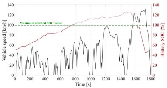
Figure 1.
SOC trajectory generated by SERCA in WLTP for a parallel P2 full HEV powertrain embedding a 1.37 kWh battery pack.
The main objective of this paper thus involves solving the drawbacks of both algorithms, i.e., reducing the computational cost of DP and allowing SERCA to comply with battery SOC physical limits. A dedicated control methodology therefore needs development to predict the near-optimal fuel economy benchmark of mild and full HEVs while ensuring computational light-weighting and compliance with SOC allowed boundaries. Additional requirements which need fulfillment in this paper involve smooth driving (e.g., related to the number of ICE activations and gear shifts) and battery lifetime. Indeed, preserving battery state-of-health (SOH) is a key requirement in electrified road vehicles [16]. It has been demonstrated how remarkably increasing the battery lifetime could indeed be achieved for mild and full HEVs at a low expense in terms of fuel consumption in the case that a proper multi-objective energy management strategy is implemented [17]. In this way, an effective downsizing of the battery pack while preserving improved fuel economy can be achieved [18].
The key idea implemented here to achieve the predefined target involves exploiting the computational rapidness of SERCA to significantly decrease the computational load of DP while preserving near-optimality in terms of fuel economy and compliance with smooth driving constraints, battery SOC constraints and battery lifetime target. The proposed HEV energy management strategy is named slope-weighted rapid dynamic programming (SRDP) and its workflow is inspired from both SERCA and DP control approaches. The novelty of the proposed SRDP approach relies in combining SERCA and DP to exploit the specific advantage of each HEV control method. SERCA is used first to rapidly identify few predefined HEV powertrain optimal operating points at each time step of the driving mission, while a DP problem is solved to optimize the HEV powertrain operation in the overall driving mission while complying with smooth driving constraints and battery SOC physical limits. Moreover, an iterative procedure allows reducing the net battery SOH variation until the considered battery lifetime requirement is met. Battery lifetime is particularly predicted here by means of a dedicated numerical battery ageing model. The rest of this paper is organized as follows: implemented numerical approaches to model the parallel P2 HEV powertrain and the high-voltage battery ageing process are described first. The following section illustrates the optimal control problem for full HEVs with constraints on smooth driving, battery SOC and battery lifetime in terms of SOH. The baseline formulation of DP for solving the retained optimal control problem is illustrated, and the reasons that restrain its practical application are discussed. The workflow of the proposed SRDP algorithm is then proposed and illustrated in detail to solve the encountered roadblock. Simulation results are finally presented, and conclusions are drawn.
2. HEV and Battery Numerical Modeling
This section describes the parallel P2 full HEV powertrain architecture first. Then, the HEV numerical modeling approach adopted in this study is discussed. Finally, the considered battery ageing model is illustrated. All the numerical models and algorithms are implemented in Matlab® software in this work.
2.1. Parallel P2 HEV Powertrain
Figure 2 illustrates the representative parallel P2 full HEV powertrain architecture retained in this study, while Table 1 lists all the corresponding relevant parameters. In this parallel P2 HEV powertrain, the electric motor/generator (MG) is placed between the ICE and the automated manual transmission (AMT) gearbox. A clutch connection is included between ICE and MG. Both ICE and MG can directly deliver tractive power to the driven wheel shaft. Two variables need to be controlled in the parallel P2 HEV powertrain retained in this work. They particularly relate to the gear number to be engaged in the AMT and to the torque split between ICE and MG. This latter control variable here corresponds to controlling the ICE torque. Indeed, in a backward HEV modelling approach such as the one described in sub-Section 2.2, controlling the ICE torque allows for automatically determining the value of MG torque required to comply with the instantaneous driver’s torque demand.
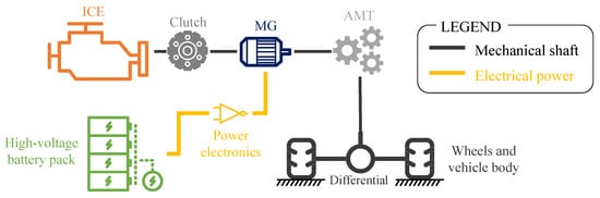
Figure 2.
Parallel P2 full HEV powertrain architecture.

Table 1.
HEV parameters.
Looking at Table 1, retained vehicle chassis data are for an A-segment passenger car and they can be found in the US EPA database [19]. The ICE data relate to a three-cylinder in-line naturally aspired spark-ignition engine, while the interior permanent magnet MG has been sized targeting a hybridization factor of around 35%. Operating maps for both the ICE and the MG have been generated by means of Amesim® software according to the procedures reported in [20,21]. A five-speed AMT configuration is retained. The modelled battery pack is assumed including quantity 240 A123 26650 cells in 120S 2P configuration, thus attaining a nominal capacity of 1.82kWh. Values of open-circuit voltage and internal resistance as a function of battery state-of-charge (SOC) have been derived from [18], retaining new cell conditions.
2.2. HEV Numerical Model
In general, a quasi-static backward modeling approach is implemented here for the HEV [22]. The requested torque at the wheels can be evaluated backwardly at each time step using Equation (1):
is the total road resistance force, which can be evaluated using experimental road load coefficients. stands for the vehicle equivalent mass evaluated at the driven wheel shaft including the inertia of the powertrain rotating components (wheels, shafts, ICE and MGs), while a is the value of vehicle acceleration as per the drive cycle requirements. is the wheel rolling radius. The total road load acting on the vehicle is expressed in Equation (2) and it is given by the rolling resistance contribution , the aerodynamic drag , the gravity’s component in the direction of motion , and which includes various other forces such as side force or transmission losses. The equation is subsequently reinterpreted highlighting the empirical road load coefficients (, and ) and their dependence from the vehicle speed. Under the assumptions of flat road and no winding, these coefficients can be experimentally derived through vehicle coast-down tests. Subsequently, they can be used to express the overall horizontal resistance force as a function of the vehicle speed. On the other hand, the contribution of needs to maintain an analytical formulation depending on the vehicle mass , the gravity acceleration g and the road slope α.
Looking at Figure 2, the torques of ICE and MG are additive and they follow Equation (3).
and are the ICE torque and the MG torque, respectively. and stand for gear ratios of the gear number engaged in the AMT () and of the final drive, respectively. Finally, and are efficiencies of the AMT and the differential, respectively. Considering the sign of as the exponential of the driveline efficiency values allows accounting for both propelling and braking cases.
Three operating modes are available for this HEV powertrain, namely pure electric, torque assist and battery charging. Different operating modes are enabled depending on whether the ICE is activated and employed to propel the vehicle or not and according to the value of . In torque assist mode, both and are positive and the overall torque provided to the transmission shaft is represented by the sum of their partial contributions. In battery charging mode, the ICE provides higher torque compared to the amount of torque requested by the driver. The exceeding torque value is then absorbed by the MG, which operates as generator to charge the battery.
As concerns the electrical energy path, the amount of power that the high-voltage battery pack is requested to either deliver or absorb () can be determined as:
where and respectively denote the mechanical power and the overall efficiency of the MG. The latter is evaluated by means of an empirical lookup table with speed () and torque () as independent variables. Retaining the sign of as exponent in the denominator allows capturing both depleting and charging battery conditions within this formula. The evolution of battery SOC over time (SOC) can then be evaluated by considering an equivalent open circuit model, as in Equation (5):
where is the battery pack capacity in ampere-seconds, while stands for the battery pack current. and are the open-circuit voltage and the internal resistance of the battery pack, as obtained by interpolating in one dimensional lookup tables with SOC and an independent variable.
Concerning the ICE, the instantaneous rate of fuel consumption in grams/second can be evaluated using an empirical steady-state lookup table with torque and speed as independent input variables.
2.3. Battery Ageing Model
A weighted ampere-hour (Ah) model has been retained from [18] and implemented in this work to estimate battery ageing. Ah models (also called performance-based models) assume that a battery can accomplish an overall lifetime Ah throughput, which is commonly weighted according to current magnitude, temperature, and other factors. These models are computationally efficient and conveniently adaptable to various battery technologies [23]. Moreover, they allow for optimizing the battery operating conditions, which is a fundamental requirement for real-time on-board implementation [24,25]. As a minor disadvantage, they are not based on the physical or chemical properties of the cell; instead, they are extrapolated from ageing tests performed under several battery operating conditions.
The battery SOH can range from 1 to 0, respectively indicating beginning and end of life. At a generic time instant ti, the battery SOH (SOH) can be evaluated using Equation (6):
where is the initial SOH, stands for the instantaneous reduction rate in SOH, and c is the instantaneous battery C-rate. c is evaluated here as the ratio between the battery power in kilowatts and the rated battery capacity in kilowatt-hours. N stands for the number of evaluated roundtrip cycles that can be achieved during the entire battery lifetime. The factor of 0.2 is correlated with the factor N being evaluated for a 20% reduction in residual capacity corresponding with a value of 0 for battery SOH. The factor of 3600 allows converting the units of c from 1/h to 1/s. N is not a constant value, but rather it depends on the battery operating conditions (i.e., temperature and C-rate). Evaluating requires determining the percentage of battery capacity loss . This can be performed by implementing the methodology introduced by Bloom et al. in 2001 [26], which takes inspiration from the Arrhenius equation describing the evolution of the chemical reaction of ideal gases. The traditional Arrhenius equation has been adapted as in Equation (7) aiming at modeling battery ageing.
The change in cell capacity is a function of an empirical pre-exponential factor , an ageing factor , the lumped cell temperature , a power-law factor and the total lifetime ampere-hour throughput . Factors and are determined based on the instantaneous battery c-rate . The numerical values for the ageing parameters of an A123 26650 LiFePO4 chemistry cell were previously determined by performing a one-year long experimental campaign. In particular, three ANR26650M1-B cells were installed in a thermal chamber and connected to a battery cycler. Three current profiles were determined by performing numerical simulations of an HEV controlled by dynamic programming in the worldwide harmonized light vehicle test procedure (WLTP). Obtained current profiles were then repeatedly fed to the battery testing cells using a 75A and 0-5 V rated channel of an MCT 75-0/5-8ME Digatron Power Electronics battery cycler. The cells were characterized in terms of residual capacity, open-circuit voltage, internal resistance, charge power capability and discharge power capability as they aged. Finally, the collected experimental data were used to calibrate the battery ageing model. The interested reader can consult [18] to obtain more details concerning the experimental campaign performed and the tuning process for the numerical ageing model. Retained values for the parameters of the described Ah battery ageing model are reported in Table 2. In particular, values for the factor reported in the third row of Table 2 correlate with the respective values of the C-rate listed in the fourth row of Table 2.
Table 2.
Parameters of the battery ageing model for A123 26650 cells.
As mentioned earlier, the battery is assumed here to reach the end of life (i.e., SOH = 0) when 20% of its initial capacity is lost. Therefore, the overall value of can be set to 20% and can be determined as a function of c and T using Equation (7). Subsequently, the total number of lifetime roundtrip cycles can be calculated using Equation (8):
where stands for the rated battery capacity in ampere-hours. The factor 2 in the denominator is to account for including both the charge and discharge ampere-hours. Figure 3 shows the number of allowed battery roundtrip cycles for different temperatures on a logarithmic scale as predicted by the illustrated ageing model.
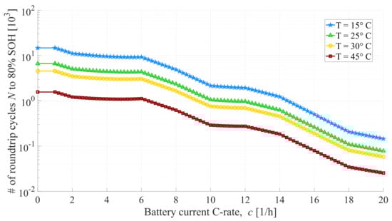
Figure 3.
Number of allowed battery roundtrip cycles as function of the C-rate and temperature as predicted by the implemented ageing model.
The described Ah numerical model is implemented in Matlab® software and it allows for predicting the battery capacity fading as a function of battery C-rate and temperature. In this work, it is assumed that ageing is independent of SOC, as supported by the ageing test results presented in [27]. This also is likely what happens for the retained case study because the HEV powertrain is studied while operating in charge sustaining mode, where the battery SOC stays within a narrow band.
3. Optimal Control of Full HEVs with Constraints on Smooth Driving, Battery SOC and Battery SOH
This section aims at describing the mathematical formulation of the optimal HEV control problem considering constraints on smooth driving, battery SOC and battery SOH. Furthermore, DP is discussed as a popular algorithm to solve the introduced control problem.
3.1. Optimal HEV Control Problem
The mathematical formulation of the optimal HEV control problem is illustrated from Equations (9)–(14). Considering discretized time instants of a predefined driving mission, this control problem aims at minimizing the cost functional expressed in Equation (9) which corresponds to the sum of the equivalent fuel consumption value in the overall drive cycle from its initial time instant to the final on . Then, optimization constraints are reported form Equations (10)–(14).
Mechanical constraints:
Battery SOC constraints:
Battery SOH constraint:
Smooth driving constraints:
Parallel P2 HEV powertrain constraints:
and stand for the average ICE efficiency in the overall drive cycle and for the fuel lower heating value, respectively. Mechanical constraints expressed in Equation (10) ensure that the HEV powertrain operation complies with the operating limits of each power component. is a binary variable that detects whether the ICE is activated or de-activated (i.e., on-1 or off-0). Equation (11) considers battery SOC constraints, where the battery SOC rate is a function of the battery SOC itself and of speed and torque values for the MG. The battery SOC value should be contained within corresponding allowed limits. Finally, charge-sustaining HEV operation is targeted by imposing similar values of battery SOC at the beginning and at the end of the driving mission while assuming an appropriate tolerance . The battery SOH constraint is considered in Equation (12) and involves guaranteeing a certain value of battery kilometrical lifetime. This is performed by assuming the same driving mission steadily repeated over the entire vehicle lifetime. and are the spatial distance driven in the overall drive cycle and the battery lifetime target, respectively. Both their values are expressed in kilometers. The factor of 0.2 is to account for 80% SOH being considered end of life. SOH is calculated using the numerical ageing model illustrated in Section 2.3 and following Equations (6)–(8). Looking at the smooth HEV driving constraints illustrated in Equation (13), the ICE torque is set to 0 when the vehicle is decelerating (i.e.,). Indeed, the noise caused by the ICE delivering positive torque could significantly undermine the riding perception when the driver aims to slow down to vehicle. Furthermore, the frequency of ICE activations and gear shifts over time in the overall driving mission should be restricted below the predefined scalar thresholds and , respectively. An ICE activation and a gear shift can be detected in those time instants in which the fuel consumption switches from zero to a positive value and the selected gear number does not match with the gear selected at the previous time instant, respectively. Finally, in a backward simulation approach the speed and torque of ICE and MG are constrained from the vehicle speed, the driver’s torque demand and the controlled values for gear number and ICE torque following the parallel P2 HEV powertrain constraints.
It should be noted that an assumption has been made in this work that considers a lumped model for the battery pack both in terms of electrical, thermal and ageing behaviors. Moreover, the battery lumped temperature has been assumed constant over time. Even if Figure 3 highlights a strong dependence of battery ageing effects on temperature, the considered representative HEV is equipped with an active battery pack cooling system which is assumed to operate in ideal conditions and to guarantee a constant battery temperature of 25 °C [17].
3.2. Baseline DP Formulation
Assuming overall a priori knowledge of future driving conditions for the drive cycle under analysis, the global optimal solution for the full HEV control problem with constraints on smooth driving, battery SOC and battery SOH can be found by exploiting the Bellman’s principle of optimality [28]. Deterministic DP can be implemented in this framework as a well-known procedure to evaluate global optimal HEV control trajectories [29,30]. In general, the optimal HEV control solution is evaluated by DP by exhaustively sweeping all possible discretized control actions while solving an optimization problem backwardly form the final time instant to the initial one of the considered driving mission [31,32]. In this work, the retained DP tool relates to the generic DP Matlab® toolbox made available by Sundstrom and Guzzella [33].
To solve an optimal control problem, DP notably requires the definition of a control variable set, a state variable set and a cost-to-go-functional. The control variable set U associated to the HEV powertrain layout retained in this study is reported in Equation (15) and it includes the gear number selection and the controlled torque of the ICE.
Combining the values of control variables comprised in U enables generating all the possible discretized HEV control actions that satisfy the constraints introduced in Equations (10)–(14). DP involves defining a state variable set X as well that comprises the variables that are tracked over time throughout the drive cycle under analysis. Constraints can be imposed both on the values of state variables at each time instant of the drive cycle and on their final values at the end of the drive cycle [34]. Equation (16) illustrates the state variable set considered for the optimal HEV control problem formulation introduced.
X includes, in this case, the battery SOC which is monitored to ensure charge-sustaining HEV operation, to comply with SOC constraints in Equation (11) and to properly evaluate SOC dependent battery parameters such as open-circuit voltage and internal resistance for example. Moreover, real-time tracking of the battery SOC value is performed on-board electrified vehicles as well [35,36]. The gear number and the ICE state are comprised in X to recognize gear-shifting and ICE de/activation events, respectively. Compliance with the smooth HEV driving constraints introduced in Equation (13) is allowed in this way. As concerns battery SOH, it needs to be tracked throughout the drive cycle to ensure that its final value fulfills the corresponding constraint expressed in Equation (12).
Finally, an instantaneous cost-to-go functional is considered as shown in Equation (17):
where the first term is the fuel consumption, while the latter two terms enable accounting for smooth driving conditions. and are constant penalization factors applied at each time instant in which gear shifting and ICE de/activation are triggered, respectively. Both and require calibration to ensure satisfaction of smooth driving constraints introduced in Equation (13) while avoiding excessive HEV fuel economy worsening. It should be noted that the DP cost functional expressed in Equation (17) does not include a net battery energy variation term as the cost functional for the optimization problem reported in Equation (9) did. This is performed in order to limit the overall number of different terms included in the DP cost functional. The overall simplicity of the algorithm can be enhanced in this way, which is beneficial for effectively handling the variety of control optimization constraints involved. Moreover, the battery energy content of the considered full HEV powertrain is limited, which overall entails small net battery energy variations at the end of a drive cycle in ideal charge-sustaining operation as predicted by DP.
The main shortcoming of DP relates to its remarkable computational cost. Moreover, the computational effort required by DP exponentially increases when increasing the number of control and state variables due to curse of dimensionality [37,38]. For this reason, the formulation of DP introduced in this section cannot be implemented on the computational platform used in this work, i.e., a desktop computer with Intel Core i7-8700 (3.2 GHz) and 32 GB of RAM. In particular, the reader can refer to [15] where the same DP formulation was applied to a parallel P2 HEV powertrain layout similar to the one considered in this work. The same DP Matlab® toolbox and the same computational platform were used. The only difference is related to the battery SOH not being involved either in the optimal control cost functional or among the DP state variables. The state variable set thus included three variables only. In these conditions, it took up to 5.8 h to complete a DP simulation considering the Worldwide-harmonized Light-vehicle Test Procedure (WLTP) as target drive cycle. The reader can notice how limits in both computational power and memory capabilities available on a desktop computer currently prevent considering a further state variable associated to battery SOH for solving the optimal HEV control problem described. Decreasing the computational load of DP is thus required for solving the optimal HEV control problem considering constraints on smooth driving, battery SOC and battery SOH.
4. Workflow of the Proposed Rapid Dynamic Programming Algorithm
Due to the increased number of considered vehicle states (i.e., battery SOC, battery SOH, selected gear number and ICE state), an optimal state-sensitive control approach such as DP may be suggested to account for their evolution over time. However, the previous section highlighted the DP limits that currently restrain its application for the considered optimal HEV control problem, i.e., excessive computational cost and the curse of dimensionality. To overcome this drawback, a rapid version of DP is proposed in this section to reduce the computational cost associated to DP and limit the related curse of dimensionality. The key idea behind the proposed approach is to consider not all the possible values of HEV powertrain control variables in terms of gear number and ICE torque at each time instant, but rather to retain only the few most efficient HEV powertrain operating points for each time step. As will be shown in the results section, this approach enables the effective application of DP for the considered optimal HEV control problem with constraints on smooth driving, battery SOC and battery SOH. Furthermore, computational efficiency and proximity with the global optimal HEV control solution can be ensured. This idea will be illustrated in detail in the follow up of this section and it has been inspired by the SERCA algorithm for controlling HEV powertrains [10,14]. For this reason, the DP-based rapid energy management approach for HEV powertrains introduced in this paper is named Slope-weighted Rapid Dynamic Programming (SRDP). Its workflow is illustrated in Figure 4 and detailed as follows.
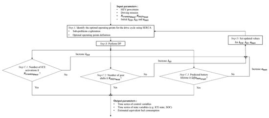
Figure 4.
Workflow of the slope-weighted rapid dynamic programming (SRDP) algorithm for HEV powertrains.
The SRDP approach receives as input, other than the HEV powertrain parameters and the driving mission under analysis, , , , and . , and are scalar coefficients that tune the ICE cranking frequency over time, the gear shit frequency over time, and the severity of the battery ageing resulting from the control actions performed, respectively. Values of , and are all initialized as 0 at the beginning of the SRDP workflow illustrated in Figure 4 not to excessively deteriorate the estimated fuel economy during the first iteration of the algorithm. Then, their values will be iteratively updated to meet HEV control optimization constraints in terms of smooth driving and battery lifetime, as will be described below for Step C.
During Step A of SRDP, the first two stages of the SERCA algorithm are performed: the sub-problems exploration and the optimal operating points definition. In the sub-problems exploration, all the possible HEV powertrain control solutions are assessed for each time instant in terms of estimated fuel consumption and use of battery energy. Then, the optimal operating points are defined in the baseline SERCA algorithms as the ones that maximize the ratio between battery SOC increase and fuel consumption [14]. However, a limited number of operating points is retained at each time instant in SRDP. Therefore, a dedicated procedure is required to adapt the selection of the optimal operating points towards reflecting the adjustment of the HEV powertrain operation to overall guarantee satisfactory battery lifetime. To this end, the approach proposed here involves adapting the definition of the slope parameter used in the baseline SERCA algorithm to identify the optimal hybrid electric operating points by including the variation in battery SOH as well. The slope parameter that characterizes the generic hybrid electric control sub-solution in a generic time instant of the drive cycle is thus expressed in Equation (18).
is the optimal pure electric operating point which can be identified as the gear number that minimizes the battery electrical energy depletion in pure electric operation for the given time instant of the driving mission. denotes a flag for battery life extension through hybrid operation compared with pure electric operation, i.e., if , while otherwise. A battery ageing sensitive slope parameter can be defined in this way that includes , i.e., the variation in the rate of battery SOH consumption between the pure electric optimal sub-solution and the hybrid electric sub-solution k. The higher the reduction in instantaneous battery capacity fading for the hybrid electric sub-solution k under analysis with respect to the optimal pure electric sub-solution for the considered time instant, the higher the corresponding value of the slope in such a manner. The coefficient allows weighting the influence of battery ageing when defining the slope values for the hybrid electric sub-solutions. Figure 5 shows an example of how the optimal hybrid electric operating points selected in a given time instant may vary when considering battery ageing as further criterion for a parallel P2 full HEV. Compared with the optimal operating points selected while considering fuel economy only (i.e., ), a shift towards lower values of instantaneous fuel consumption and battery charged energy can be observed for the optimal hybrid electric operating points for both gears when retaining battery ageing as well (e.g., ). This correlates well with the overall rate of battery capacity fading being proportional to the battery depth of charge and discharge in the retained driving mission.
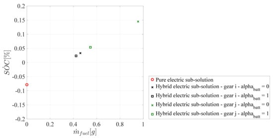
Figure 5.
Example of battery SOH sensitive sub-solutions comparison for a sub-problem in SRDP (v = 27.5 km/h, a = 0.3 m/s2).
Step A in Figure 4 leads to identify a limited number of suitable optimal operating points for each time instant of the retained driving mission. A variable with the structure illustrated in Table 3 can thus be created that contains the set of values for control variables u and state variables related to each of the N+1 operating points identified at the generic time instant i. In the next sub-section, a case study will be presented to determine the number N+1 and the classification of the optimal operating points retained through SERCA for each time instant of the retained driving mission.
Table 3.
Stored variable for the target drive cycle in SRDP.
Only the variable illustrated in Table 3 is then considered as input for the control variable set in DP executed at Step B in Figure 4. This method allows us to remarkably shrink the search space that the DP is required to exhaustively explore for the driving mission under analysis. The state variables considered here in SRDP are the battery SOC, the ICE state and the selected gear number. On the other hand, the instantaneous cost functional whose value integrated throughout the considered driving mission needs minimization by SRDP for a parallel P2 HEV can be expressed in Equation (19).
Three additional terms are included to the instantaneous fuel consumption in the expression of the SRDP cost functional that enable reducing the number of ICE activations and gear shifts and increasing the battery lifetime, respectively. and are variables that can detect ICE cranking and gear shift events thanks to changes in the values of corresponding state variables, respectively. Once the traditional workflow of DP has been completed, Step C of SRDP aims to ensure that both smooth driving and battery lifetime set criteria are satisfied by the generated control solution. This relates to the number of ICE activations being less than or equal to , the number of gear shifts being less than or equal to , and the kilometrical battery lifetime being equal to or greater than . The workflow of SRDP is concluded in case all the three listed conditions are satisfied at once. Alternatively, weighting coefficients related to the unsatisfied criteria are updated accordingly in Step D in Figure 4. Particularly, is increased to reduce the number of ICE activations, is increased to reduce the number of gear shifts and is increased to extend battery lifetime in case the corresponding criteria have not been fulfilled in the concluded iteration of SRDP. It should be reminded that battery SOC constraints are already straightforwardly fulfilled in SRDP by imposing appropriate constraints both on the instantaneous and on the final values of the corresponding state variable. On the other hand, a dedicated approach is proposed to extend the battery lifetime in SRDP through increasing the value of , since the battery SOH is not included in the retained state variables.
Steps A to D of SRDP can thus be recursively performed until all the smooth drivability and battery lifetime criteria have been satisfied. After completion of the SRDP algorithm, the output parameters of the algorithm in Figure 4 include time series of control variables, time series of state variables and the estimated fuel consumption for the analysed driving mission. A case study to determine the most suitable number and category of hybrid electric operating points at each time instant will be presented in the next section. Then, a comparison between SRDP and baseline DP will be discussed over different driving missions.
5. Simulation Results
A case study to determine the most suitable number and category of hybrid electric operating points at each time instant is presented in this section. Then, a comparison between SRDP and baseline DP with the full set of control variable values will be discussed over different driving missions.
5.1. Definition of Number and Type of Selected Hybrid Electric Optimal Operating Points
Step A of the SRDP workflow illustrated in Figure 4 involves identifying and selecting at each time instant the optimal operating points to be considered for hybrid electric mode. Once the given N hybrid electric points are defined at each time instant, these can then be stored in the variable illustrated in Table 3 and constituted by a number of rows equal to the number of time instants of the driving mission and a number of columns equal to N+1 corresponding to the pure electric optimal operating point and the N hybrid electric operating points as defined by SERCA. In this framework, a comparative study needs execution in order to determine the number and type of hybrid electric points selected at each time instant of the driving mission. In case of stepped gear transmission HEVs, SERCA generally identifies one optimal hybrid electric operating point for each operable gear number of the transmission based on the value of the slope parameter [14]. However, multiple optimal operating points may be considered as well in SRDP to enhance the effectiveness of the algorithm when accounting for battery SOH sensitivity as well in the HEV operation. The additional hybrid electric operating points may be identified in this case according to the ranking of the slope values (e.g., the second-best slope value and the third-best slope value). Furthermore, storing optimal operating points for each gear number of the stepped gear transmission HEV at each time instant may reveal a redundant and computationally inefficient approach in this case, since only a limited number of gears typically operate in the most efficient conditions depending on the values of speed and acceleration request for the sub-problem under analysis. However, a certain minimum number of available gears may require consideration at each time instant in order to effectively reduce the number of gear shifts operated throughout the entire driving mission.
To contribute solving the aforementioned uncertainties, a case study is performed assessing different numbers of retained gears and optimal operating points per gear. The main objective is to determine the most appropriate value of , i.e., the number of sub-optimal operating points that SERCA needs to select at each time instant of the drive cycle under analysis. Only the identified points will then be processed by the DP to identify the optimal HEV control trajectory over the entire drive cycle. The overall number of selected operating points at each time instant depends on two main factors:
- The number of gears considered. For example, if only one gear is considered, its value will be selected at each time instant as the one linked to the optimal hybrid electric point #1 for the corresponding row in Table 3. If more than one gear is considered, the additional gear numbers in each time instant are identified looking at the sub-sequent optimal hybrid electric points (e.g., #2, #3 and following ones) in the corresponding row in Table 3.
- The number of optimal hybrid electric points considered per gear. Two categories of hybrid electric points are considered here. The first one includes the θ operating points identified by maximizing the SERCA slope parameter defined in Equation (18). The second category involves a single operating point per gear which is identified by interpolating in the ICE optimal operating line (OOL), i.e., the line of operating points that minimize the fuel rate for any given value of ICE mechanical power.
The best option needs therefore to be defined among the several possibilities that are available in terms of for the proposed SRDP approach depending on both the number of retained gears and the number of optimal hybrid electric points considered per gear. Near-optimality in the estimated equivalent fuel consumption and computational light-weighting are here the two metrics for identifying the best SRDP option. The following options have particularly been considered for the SRDP based HEV off-line energy management strategy in terms of the number of retained gears and the number of optimal hybrid electric points considered per gear for the retained HEV powertrain:
- Full set of control variable values in terms of gear number and ICE torque, i.e., without pre-identifying optimal operating points with SERCA (baseline ‘DP’). Considering an ICE torque discretization step of 5 Nm, 22 elements are required to cover the range from 0 Nm to the maximum allowed ICE torque value (90 Nm in this case) and to retain an extra term for pure electric operation. For a 5 gears P2 HEV layout, 110 elements therefore define the discretized control variable set U in the baseline DP approach (i.e., ).
- (3 gears) × (4 θ points + 1 ICE OOL point). This leads to consider a total of 16 operating points ( = 16) in the control variable set of SRDP (i.e., 1 pure electric point, 12 SERCA hybrid electric points and 3 ICE OOL points).
- (3 gears) × (3 θ points + 1 ICE OOL point). This leads to consider a total of 13 operating points ( = 13) in the control variable set of SRDP (i.e., 1 pure electric point, 9 SERCA hybrid electric points and 3 ICE OOL points).
- (3 gears) × (2 θ points + 1 ICE OOL point). This leads to consider a total of 10 operating points ( = 10) in the control variable set of SRDP (i.e., 1 pure electric, 6 SERCA hybrid electric points and 3 ICE OOL points).
- (3 gears) × (1 θ point + 1 ICE OOL point). This leads to consider a total of 7 operating points ( = 7) in the control variable set of SRDP (i.e., 1 pure electric, 3 SERCA hybrid electric points and 3 ICE OOL points).
- (3 gears) × (4 θ points). This leads to consider a total of 13 operating points ( = 13) in the control variable set of SRDP (i.e., 1 pure electric point and 12 SERCA hybrid electric points).
- (2 gears) × (4 θ points + 1 ICE OOL point). This leads to consider a total of 11 operating points ( = 11) in the control variable set of SRDP (i.e., 1 pure electric point, 8 SERCA hybrid electric points and 2 ICE OOL points).
- (2 gears) × (3 θ points + 1 ICE OOL point). This leads to consider a total of 9 operating points ( = 9) in the control variable set of SRDP (i.e., 1 pure electric point, 6 SERCA hybrid electric points and 2 ICE OOL points).
- (2 gears) × (2 θ points + 1 ICE OOL point). This leads to consider a total of 7 operating points ( = 7) in the control variable set of SRDP (i.e., 1 pure electric point, 4 SERCA hybrid electric points and 2 ICE OOL points).
- (2 gears) × (1 θ point + 1 ICE OOL point). This leads to consider a total of 5 operating points ( = 5) in the control variable set of SRDP (i.e., 1 pure electric point, 2 SERCA hybrid electric points and 2 ICE OOL points).
- (3 gears) × (1 ICE OOL point). This leads to consider a total of 4 operating points ( = 4) in the control variable set of SRDP (i.e., 1 pure electric point and 3 ICE OOL points).
Each of the 11 listed HEV energy management approaches consider the same state variable set which includes gear number, ICE state and battery SOC. Each version of the SRDP algorithm is evaluated in WLTP considering the HEV powertrain data and layout presented in Section 2 and reported in Table 1.
The ICE is set here not to deliver positive torque in the time instants of the driving mission in which the output torque is negative, i.e., only pure electric operation or hybrid electric operation with ICE idling are available. In this case, the discretized vector for the ICE torque is converted into a vector having the same number of elements and containing different values for the MG negative torque at different gears. Regulating the blending between MG regenerative torque and friction brake torque is enabled in this way to allow the DP optimizer selecting the best control actions in terms of electrical energy recovery and battery lifetime preservation throughout the retained driving mission. The state variable related to battery SOC has been discretized with 251 elements ranging from 0.3 to 0.9, while the initial battery SOC has been set to 0.6. is assumed here being 300 thousand kilometers [17]. Finally, values of and have been set to 0.7 and 3.6 per minute of driving, respectively [15].
In order to identify the best option for SRDP control variables among the 10 listed above, simulations have been performed for the retained P2 HEV layout in WLTP being controlled off-line. The SRDP procedure has been particularly interrupted in case the battery lifetime and smooth drivability requirements had not been met after the 20th iteration of Step A to Step D of the algorithm. Obtained results in terms of estimated fuel consumption, battery lifetime, number of ICE activations, number of gear shifts and CT have been reported in Table 4 together with corresponding results for the normal DP.
Table 4.
Results in WLTP for options of SRDP control variable set in terms of estimated equivalent fuel consumption (EFC), battery lifetime, ICE activations, gear shifts, number of algorithm iterations (nITER) and computational time (CT) considering a desktop computer with Intel Core i7-8700 (3.2 GHz) and 32 GB of RAM.
The baseline DP with full set of control variables requires 38 min to complete a single iteration on a desktop computer with Intel Core i7-8700 (3.2 GHz) and 32 GB of RAM, and 3 iterations are demanded to satisfy all the considered battery lifetime and smooth drivability requirements. On the other hand, significantly lower values of computational time are required to complete an iteration of SRDP (i.e., ranging from 5 min to 11 min), while a higher number of iterations nITER need to be performed (i.e., ranging from 4 to 12). More iterations may particularly be required to compensate for the decreased number of hybrid electric operating points available for each time instant of the considered driving mission in Step B of SRDP. Only two SRDP cases are found not complying with imposed battery lifetime and smooth drivability criteria once the maximum number of allowed iterations for the algorithm is reached. Unsuccessful options for the SRDP control variable set particularly relate to case 6 in which the operating points of the ICE OOL are not considered, and to case 11 in which the optimal hybrid electric operating points identified through the SERCA approach are not considered. Both the listed options have consequently been discarded. This suggests that combining hybrid electric operating points identified through SERCA (i.e., by optimizing the overall operation of the electrified propulsion system) with points identified through the ICE OOL may be a viable approach. In general, the SRDP estimated fuel consumption increase compared with DP is limited within 8.1%, while the corresponding computational time in most SRDP cases is reduced by 50% to 80% despite the slightly increased number of iterations. The effectiveness of the proposed SRDP approach in limiting the EFC increase with respect to the global optimal HEV control solution while consistently reducing the computational cost may be suggested in this way. Figure 6 illustrates the Pareto frontier for the options of SRDP control variable set assessed in terms of WLTP EFC increase compared with DP and computational time normalized according to the DP corresponding value. In general, lower values of computational time are required for the SRDP options retaining 2 gears only compared with the SRDP options retaining 3 gears, while the estimated fuel consumption increase as a function of the different options for the SRDP control variable set does not show a uniformed trend. A global optimal option can be clearly identified for the SRDP control variable set that achieves simultaneous minimization of the normalized computational time and the estimated equivalent fuel consumption increase with respect to DP. This particularly corresponds to the test case number 4, i.e., SRDP with 10 elements in the control variable set involving the best 3 gears at each time instant, and the 2 best hybrid electric operating points and the ICE OOL point per gear. The identified option appears producing a HEV control solution comparable with the one from DP in terms of estimated fuel consumption, battery lifetime, number of ICE activations and number of gear shifts while reducing the corresponding computational time by around 78%. In the next sub-section, a case study will be conducted assessing the performance of the identified option for the SRDP control variable set in various driving missions.
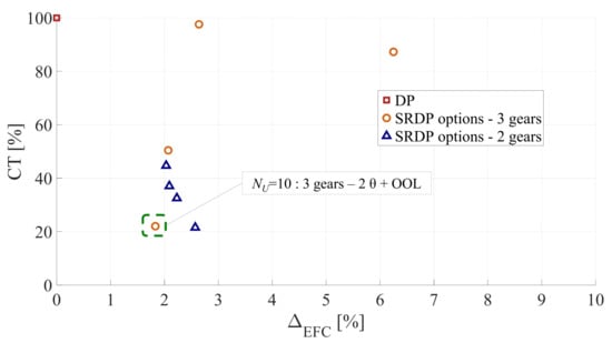
Figure 6.
Pareto frontier for options of SRDP control variable set in terms of WLTP estimated equivalent fuel consumption percentage increase () and percentage computational time (CT) compared with DP.
5.2. Case Study: SRDP for a Full HEV
Once retaining 3 gears and 2 slope points with an ICE OOL point per gear at each time instant has been identified as the best option for the SRDP control variable set, the performance of the developed SRDP algorithm is assessed in this sub-section over various driving missions. Values of estimated fuel consumption and predicted battery lifetime, number of ICE activations and gear shifts and required computational time obtained from the SRDP are particularly benchmarked with the corresponding results for the baseline DP that consider the full set of control variable values in terms of gear number and ICE torque. Both SRDP and DP here consider three state variables, namely the gear number, the ICE state and the battery SOC. Retained driving missions in this case include the New European Drive Cycle (NEDC), the Urban Dynamometer Driving Schedule (UDDS), the Highway Federal Test Procedure (HWFET), the WLTP and the US06 Supplemental Federal Test Procedure (US06). Table 5 summarizes the obtained results for both HEV control algorithms in the considered driving missions, while times series of cumulated fuel consumption, battery SOC, battery SOH and gear shifting along with ICE operating points for each driving mission have been illustrated in Figure A1, Figure A2, Figure A3, Figure A4 and Figure A5 in Appendix A. These plots can help the reader to get more insight in the HEV powertrain control solutions identified by both DP and SRDP. Despite both SRDP and DP provide comparable values of estimated fuel consumption over the entire drive cycles (denoted by the final values of cumulated fuel consumption in sub-figures a in Figure A1, Figure A2, Figure A3, Figure A4 and Figure A5), the two algorithms entail different HEV powertrain operations. This especially holds for WLTP and UDDS drive cycles respectively in Figure A1 and Figure A4, where the time series of battery SOC (sub-figures b), battery SOH (sub-figures d), gear shifting (sub-figures e) notably differ between DP and SRDP. In general, looking at sub-figures c in Figure A1, Figure A2, Figure A3, Figure A4 and Figure A5, the ICE operating points set by DP are spread near the best ICE efficiency region. As concerns SRDP, a similar behaviour can be observed while it should be noted that several selected ICE operating points are located on the OOL. This corroborates the effectiveness of considering operating points of the ICE OOL in the proposed SRDP HEV control approach.
Table 5.
Comparing SRDP with DP in terms of estimated equivalent fuel consumption (EFC), battery lifetime, ICE activation frequency, gear shift frequency and computational time (CT) over various driving missions.
Looking at results reported in Table 5, it can be seen how both SRDP and DP comply with imposed constraints in terms of battery lifetime, frequency of ICE activations and gear shifts over time in all the drive cycles considered. On average, the increase in estimated fuel consumption for SRDP is limited in this case to 1.4% compared to DP over the retained drive cycles, while on average the corresponding SRDP computational cost is reduced by 55.9% with respect to DP. Despite in general the values of computational time associated to SRDP increases compared with the ones associated to the SERCA algorithm (i.e., 1 to 5 min per drive cycle using the same computational platform), it should be noted that the developed SRDP approach allows complying with battery SOC boundaries for full HEVs while ensuring compliance with smooth driving and battery lifetime requirements set.
Overall, the proposed SRDP algorithm exhibits the highest performance when benchmarking with the baseline DP in NEDC, UDDS and HWFET cycles. This corresponds to the fuel consumption estimated by SRDP in Table 5 being only 0.8%, 0.3% and 0.7% higher compared with DP, respectively. Moreover, it should be noted that values of battery lifetime predicted by SRDP in NEDC, UDDS and HWFET are 8.2%, 5.4% and 1.5% higher than the corresponding values obtained using the baseline DP approach, respectively. This contributes to further narrow the difference in the performance between the two algorithms. On the other hand, slightly lower performance can be observed for the proposed SRDP algorithm in WLTP and US06 cycles. This may relate to both cycles being known for entailing more dynamic and demanding vehicle driving conditions in terms of speed and traction power. Especially for the US06 cycle, the reader can refer to Figure A5c, where the ICE operating points are more scattered and located in higher power regions compared with corresponding sub-figures c for the remaining drive cycles shown in Figure A1, Figure A2, Figure A3 and Figure A4 in the Appendix A. This notably increases the difficulty encountered by SRDP in replicating the optimal HEV operation predicted by the baseline DP while reducing the computational load thanks to limiting the number of HEV operating points considered.
6. Conclusions
Effective energy management is a crucial aspect in HEVs. An appropriate HEV powertrain control approach must guarantee enhanced fuel economy while simultaneously complying with constraints on battery SOC, battery SOH and smooth driving in terms of limited frequencies of ICE activations and gear shifts over time. Furthermore, the overall computational efficiency of the control algorithm needs to be preserved. This paper has presented a rapid DP based energy management strategy for full HEVs which is named Slope-weighted Rapid Dynamic Programming (SRDP). SRDP combines the computational efficiency of the SERCA algorithm with DP as an effective approach to ensure compliance with battery SOC constraints. Similarly as SERCA, SRDP considers only the most efficient HEV powertrain operating points at each time instant of the drive cycle. This is significantly beneficial for computational efficiency. A case study performed for a full parallel P2 HEV demonstrates that SRDP can effectively comply with battery lifetime and smooth driving constraints, while limiting the estimated fuel consumption increase within 3.3% compared with the baseline DP. Moreover, SRDP can attain notable savings in terms of computational cost that range within 43% and 78% compared with the baseline DP.
The presented formulation of SRDP is general and it can be applied to any available DP approach and available toolbox to enhance the computational efficiency of the overall HEV powertrain control algorithm. Given the computational advantage and the demonstrated near-optimality in terms of estimated fuel consumption, SRDP is a suitable candidate as rapid energy management strategy to be employed in HEV powertrain design and sizing methodologies. In particular, the computational efficiency of SRDP can be exploited to effectively explore the large design space associated with HEV powertrains. Moreover, SRDP could be employed as a predictive powertrain controller on-board HEVs. In particular, SRDP could be interfaced with a future vehicle velocity predictor to extract optimal HEV control trajectories for near-future powertrain operation. Related future work can pursue these directions.
Funding
This research was funded by the Doctoral School of Politecnico di Torino.
Institutional Review Board Statement
Not applicable.
Informed Consent Statement
Not applicable.
Data Availability Statement
Not applicable.
Conflicts of Interest
The author declares no conflict of interest.
Abbreviations
| AMT | Automated manual transmission |
| DP | Dynamic programming |
| EFC | Equivalent fuel consumption |
| MG | Electric motor/generator |
| HEV | Hybrid electric vehicle |
| HWFET | Highway federal test procedure |
| ICE | Internal combustion engine |
| NEDC | New European Drive Cycle |
| OOL | Optimal operating line |
| P2 HEV | Parallel P2 hybrid electric vehicle |
| SOC | State-of-charge |
| SOH | State-of-health |
| SRDP | Slope-weighted Rapid Dynamic Programming |
| UDDS | Urban dynamometer driving schedule |
| US06 | US06 supplemental procedure |
| WLTP | Worldwide harmonized light-vehicle test procedure |
Appendix A. Time Series of Control and State Variables Generated by DP and SRDP for a P2 Full HEV
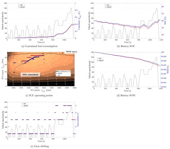
Figure A1.
Time series of control and state variables and ICE operating points for the P2 full HEV controlled by DP and SRDP in NEDC cycle.
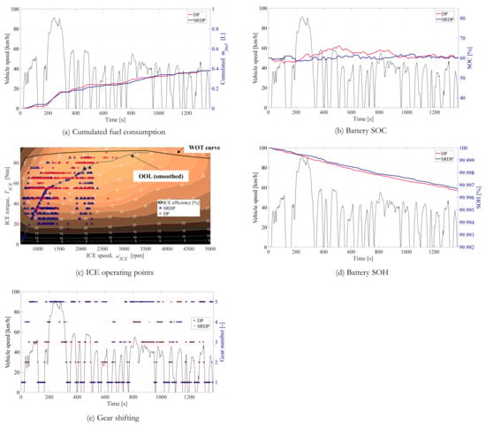
Figure A2.
Time series of control and state variables and ICE operating points for the P2 full HEV controlled by DP and SRDP in UDDS cycle.
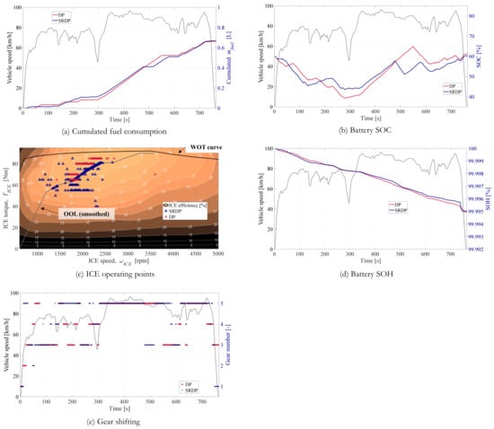
Figure A3.
Time series of control and state variables and ICE operating points for the P2 full HEV controlled by DP and SRDP in HWFET cycle.
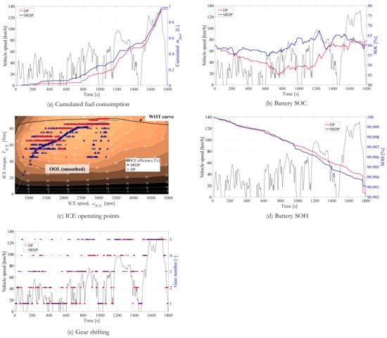
Figure A4.
Time series of control and state variables and ICE operating points for the P2 full HEV controlled by DP and SRDP in WLTP cycle.
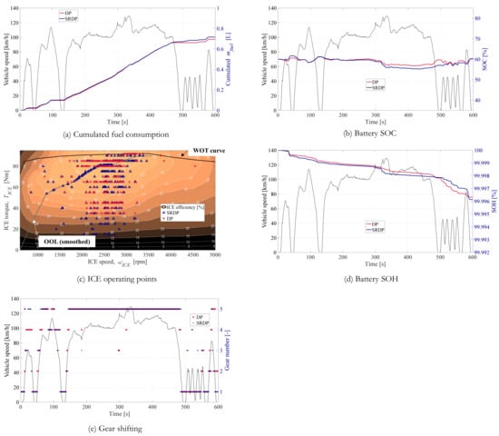
Figure A5.
Time series of control and state variables and ICE operating points for the P2 full HEV controlled by DP and SRDP in US06 cycle.
References
- Matsumoto, K.; Nakamine, Y.; Eom, S.; Kato, H. Demographic, Social, Economic, and Regional Factors Affecting the Diffusion of Hybrid Electric Vehicles in Japan. Energies 2021, 14, 2130. [Google Scholar] [CrossRef]
- Xue, Q.; Zhang, X.; Teng, T.; Zhang, J.; Feng, Z.; Lv, Q. A Comprehensive Review on Classification, Energy Management Strategy, and Control Algorithm for Hybrid Electric Vehicles. Energies 2020, 13, 5355. [Google Scholar] [CrossRef]
- Musa, A.; Pipicelli, M.; Spano, M.; Tufano, F.; De Nola, F.; Di Blasio, G.; Gimelli, A.; Misul, D.A.; Toscano, G. A Review of Model Predictive Controls Applied to Advanced Driver-Assistance Systems. Energies 2021, 14, 7974. [Google Scholar] [CrossRef]
- Biswas, A.; Emadi, A. Energy management systems for electrified powertrains: State-of-the-art review and future trends. IEEE Trans. Veh. Technol. 2019, 68, 6453–6467. [Google Scholar] [CrossRef]
- Ali, A.M.; Söffker, D. Towards Optimal Power Management of Hybrid Electric Vehicles in Real-Time: A Review on Methods, Challenges, and State-Of-The-Art Solutions. Energies 2018, 11, 476. [Google Scholar] [CrossRef] [Green Version]
- Yuan, Z.; Teng, L.; Fengchun, S.; Peng, H. Comparative Study of Dynamic Programming and Pontryagin’s Minimum Principle on Energy Management for a Parallel Hybrid Electric Vehicle. Energies 2013, 6, 2305–2318. [Google Scholar] [CrossRef]
- Bellman, R.; Lee, E. History and development of dynamic programming. IEEE Control Syst. Mag. 1984, 4, 24–28. [Google Scholar] [CrossRef]
- van Harselaar, W.; Schreuders, N.; Hofman, T.; Rinderknecht, S. Improved implementation of dynamic programming on the example of hybrid electric vehicle control. IFAC-Pap. 2019, 52, 147–152. [Google Scholar] [CrossRef]
- Raphael, C. Coarse-to-fine dynamic programming. IEEE Trans. Pattern Anal. Mach. Intell. 2001, 23, 1379–1390. [Google Scholar] [CrossRef]
- Anselma, P.G.; Biswas, A.; Belingardi, G.; Emadi, A. Rapid assessment of the fuel economy capability of parallel and series-parallel hybrid electric vehicles. Appl. Energy 2020, 275, 115319. [Google Scholar] [CrossRef]
- Arvidsson, R.; McKelvey, T. Comparing Dynamic Programming Optimal Control Strategies for a Series Hybrid Drivetrain; SAE Technical Paper 2017-01-2457; SAE: Warrendale, PA, USA, 2017. [Google Scholar]
- Shankar, R.; Marco, J.; Assadian, F. The Novel Application of Optimization and Charge Blended Energy Management Control for Component Downsizing within a Plug-in Hybrid Electric Vehicle. Energies 2012, 5, 4892–4923. [Google Scholar] [CrossRef]
- Kim, K.; Kim, N.; Jeong, J.; Min, S.; Yang, H.; Vijayagopal, R.; Rousseau, A.; Cha, S.W. A Component-Sizing Methodology for a Hybrid Electric Vehicle Using an Optimization Algorithm. Energies 2021, 14, 3147. [Google Scholar] [CrossRef]
- Anselma, P.G.; Huo, Y.; Roeleveld, J.; Belingardi, G.; Emadi, A. Slope-weighted energy-based rapid control analysis for hybrid electric vehicles. IEEE Trans. Veh. Technol. 2019, 68, 4458–4466. [Google Scholar] [CrossRef]
- Anselma, P.G. Computationally efficient evaluation of fuel and electrical energy economy of plug-in hybrid electric vehicles with smooth driving constraints. Appl. Energy 2022, 307, 118247. [Google Scholar] [CrossRef]
- Bonfitto, A. A Method for the Combined Estimation of Battery State of Charge and State of Health Based on Artificial Neural Networks. Energies 2020, 13, 2548. [Google Scholar] [CrossRef]
- Anselma, P.G.; Kollmeyer, P.; Belingardi, G.; Emadi, A. Multi-Objective Hybrid Electric Vehicle Control for Maximizing Fuel Economy and Battery Lifetime. In Proceedings of the 2020 IEEE Transportation Electrification Conference & Expo (ITEC), Chicago, IL, USA, 23–26 June 2020; pp. 1–6. [Google Scholar]
- Anselma, P.G.; Kollmeyer, P.; Lempert, J.; Zhao, Z.; Belingardi, G.; Emadi, A. Battery state-of-health sensitive energy management of hybrid electric vehicles: Lifetime prediction and ageing experimental validation. Appl. Energy 2021, 285, 116440. [Google Scholar] [CrossRef]
- United States Environmental Protection Agency. Compliance and Fuel Economy Data—Annual Certification Data for Vehicles, Engines, and Equipment. Available online: https://www.epa.gov/compliance-and-fuel-economy-data/annual-certification-data-vehicles-engines-and-equipment (accessed on 20 January 2022).
- Alix, G.; Dabadie, J.; Font, G. An ICE Map Generation Tool Applied to the Evaluation of the Impact of Downsizing on Hybrid Vehicle Consumption; SAE Technical Paper 2015-24-2385; SAE: Warrendale, PA, USA, 2015. [Google Scholar]
- le Berr, F.; Abdelli, A.; Postariu, D.-M.; Benlamine, R. Design and Optimization of Future Hybrid and Electric Propulsion Systems: An Advanced Tool Integrated in a Complete Workflow to Study Electric Devices. Oil Gas Sci. Technol. 2012, 67, 547–562. [Google Scholar] [CrossRef] [Green Version]
- Kapetanović, M.; Vajihi, M.; Goverde, R.M.P. Analysis of Hybrid and Plug-In Hybrid Alternative Propulsion Systems for Regional Diesel-Electric Multiple Unit Trains. Energies 2021, 14, 5920. [Google Scholar] [CrossRef]
- Meis, C.; Mueller, S.; Rohr, S.; Kerler, M.; Lienkamp, M. Guide for the Focused Utilization of Aging Models for Lithium-Ion Batteries—An Automotive Perspective. SAE Int. J. Passeng. Cars-Electron. Electr. Syst. 2015, 8, 195–206. [Google Scholar] [CrossRef]
- Yang, Z.; Mamun, A.; Makam, S.; Okma, C. An Empirical Aging Model for Lithium-Ion Battery and Validation Using Real-Life Driving Scenarios; SAE Technical Paper 2020-01-0449; SAE: Warrendale, PA, USA, 2020. [Google Scholar]
- Anselma, P.G.; Del Prete, M.; Belingardi, G. Battery High Temperature Sensitive Optimization-Based Calibration of Energy and Thermal Management for a Parallel-through-the-Road Plug-in Hybrid Electric Vehicle. Appl. Sci. 2021, 11, 8593. [Google Scholar] [CrossRef]
- Bloom, I.; Cole, B.W.; Sohn, J.J.; Jones, S.A.; Polzin, E.G.; Battaglia, V.S.; Henriksena, G.L.; Motlochb, C.; Richardsonb, R.; Unkelhaeuserc, T.; et al. An accelerated calendar and cycle life study of Li-ion cells. J. Power Sources 2001, 101, 238–247. [Google Scholar] [CrossRef]
- Wang, J.; Liu, P.; Hicks-Garner, J.; Sherman, E.; Soukiazian, S.; Verbrugge, M.; Tataria, H.; Musser, J.; Finamore, P. Cycle-life model for graphite-LiFePO4 cells. J. Power Sources 2011, 196, 3942–3948. [Google Scholar] [CrossRef]
- Bellman, R.; Kalaba, R. Dynamic programming and adaptive processes: Mathematical foundation. IRE Trans. Autom. Control 1960, AC-5, 5–10. [Google Scholar] [CrossRef]
- Lempert, J.; Vadala, B.; Arshad-Aliy, K.; Roeleveld, J.; Emadi, A. Practical Considerations for the Implementation of Dynamic Programming for HEV Powertrains. In Proceedings of the 2018 IEEE Transportation Electrification Conference and Expo (ITEC), Long Beach, CA, USA, 13–15 June 2018; pp. 755–760. [Google Scholar]
- Bruck, L.; Lempert, A.; Amirfarhangi Bonab, S.; Lempert, J.; Biswas, A.; Anselma, P.G.; Roeleveld, J.; Rane, O.; Madireddy, K.; Wasacz, B.; et al. A Dynamic Programming Algorithm for HEV Powertrains Using Battery Power as State Variable; SAE Technical Paper 2020-01-0271; SAE: Warrendale, PA, USA, 2020. [Google Scholar]
- Miretti, F.; Misul, D.; Spessa, E. DynaProg: Deterministic Dynamic Programming solver for finite horizon multi-stage decision problems. SoftwareX 2021, 14, 100690. [Google Scholar] [CrossRef]
- Spano, M.; Anselma, P.G.; Misul, D.A.; Belingardi, G. Exploitation of a Particle Swarm Optimization Algorithm for Designing a Lightweight Parallel Hybrid Electric Vehicle. Appl. Sci. 2021, 11, 6833. [Google Scholar] [CrossRef]
- Sundstrom, O.; Guzzella, L. A generic dynamic programming Matlab function. In Proceedings of the 2009 IEEE Control Applications, (CCA) & Intelligent Control, (ISIC), St. Petersburg, Russia, 8–10 July 2009; pp. 1625–1630. [Google Scholar]
- Elbert, P.; Ebbesen, S.; Guzzella, L. Implementation of Dynamic Programming for n-Dimensional Optimal Control Problems with Final State Constraints. IEEE Trans. Control Syst. Technol. 2013, 21, 924–931. [Google Scholar] [CrossRef]
- Luciani, S.; Feraco, S.; Bonfitto, A.; Tonoli, A. Hardware-in-the-Loop Assessment of a Data-Driven State of Charge Estimation Method for Lithium-Ion Batteries in Hybrid Vehicles. Electronics 2021, 10, 2828. [Google Scholar] [CrossRef]
- Luciani, S.; Feraco, S.; Bonfitto, A.; Tonoli, A.; Amati, N.; Quaggiotto, M. A Machine Learning Method for State of Charge Estimation in Lead-Acid Batteries for Heavy-Duty Vehicles. In Proceedings of the ASME 2021 International Design Engineering Technical Conferences and Computers and Information in Engineering Conference. Volume 1: 23rd International Conference on Advanced Vehicle Technologies (AVT), Virtual, Online, 17–19 August 2021; American Society of Mechanical Engineers: New York, NY, USA, 2021. [Google Scholar]
- Wang, S.; Jiang, Z.; Liu, Y. Dimensionality Reduction Method of Dynamic Programming under Hourly Scale and Its Application in Optimal Scheduling of Reservoir Flood Control. Energies 2022, 15, 676. [Google Scholar] [CrossRef]
- Anselma, P.G. Optimization-Driven Powertrain-Oriented Adaptive Cruise Control to Improve Energy Saving and Passenger Comfort. Energies 2021, 14, 2897. [Google Scholar] [CrossRef]
Publisher’s Note: MDPI stays neutral with regard to jurisdictional claims in published maps and institutional affiliations. |
© 2022 by the author. Licensee MDPI, Basel, Switzerland. This article is an open access article distributed under the terms and conditions of the Creative Commons Attribution (CC BY) license (https://creativecommons.org/licenses/by/4.0/).