1. Introduction
Today’s goal to reduce carbonization of electrical power systems aids the significant penetration of distributed energy resources with an expectation to achieve, in the European Union (EU), a total share of 27% of renewable generation and a reduction of 40% of greenhouse gases by 2030 [
1]. The integration of renewable energy sources and the increasing number of regular consumers that become prosumers transform the old centralized, unidirectional electricity grid into a more decentralized grid with bidirectional energy and communication flow [
2]. As such, the existence of prosumers enables the concept of energy sharing in an energy community, where these entities can share their surplus of energy with other members [
3]. This provides the opportunity for end-users in citizen energy communities (CEC) to be critical players in the energy sector, further contributing to the supply-demand balance by having more active participation, not only as prosumers but also by participating in demand response (DR) programs. Demand response can be defined as actively altering the normal energy consumption habits of end-users in reaction to variations in electricity prices, or in response to incentives to reduce consumption during high wholesale market prices, or when the systems dependability is compromised [
4].
Participation in DR programs helps integrate electric loads and renewable energy sources cost-effectively [
5]. In this context, end-users represent a potential source of energy flexibility and, by engaging in DR programs, can play a significant role in the transition to the decarbonization of energy systems, resulting in a clean energy future [
6]. From a technology perspective, energy flexibility procurement can be done through the usage of internet of things (IoT) devices integrated into residential households, transforming them into smart homes, maximizing user comfort while minimizing the cost of electricity [
7]. These smart homes are linked in a smart community through IoT devices, measuring and communicating detailed energy consumption information to energy management systems [
8]. These management systems can precisely control individual home appliances via the use of power meters or smart plugs, operating in response to DR programs [
9]. In this context, the application of clustering algorithms is important since they can facilitate the analysis of large amounts of data collected from smart meters [
10].
Previous studies, such as [
11,
12], already present methodologies oriented towards end-user participation in DR events. In [
11], a method is presented in which end-users are assigned a trustworthy rank according to their past participation experience. In this way, the aggregator would invite those with the highest trustworthy rank to participate in the DR event. However, since this ranking only depends on past participation, it is not possible for an end-user who missed some DR events to improve their ranking. In [
12], a model based on clustering algorithms is presented to cluster several loads with similar consumption patterns to improve the DR events’ accuracy. Moreover, in order to incentivize participation, this study considers that the largest clusters have the lowest DR application costs. In this way, the cluster with lower DR application costs is prioritized during the DR event. The results demonstrated that end-users were compensated accordingly to their participation, reducing their electricity bills. Nonetheless, the study in [
12] has its limitations regarding how it ranks the loads, where smaller clusters are penalized.
This paper proposes a novel methodology based on clustering algorithms for end-user participation in DR events in CEC. Considering the previous studies, the novelty of the presented methodology is ranking the end-users through the combination of three metrics based on clustering algorithms. This enables the correct selection of end-users to be invited to the DR program. With the combination of these three metrics, the end-users can have more opportunities to participate in DR events since the presented ranking is based on different types of end-user data, namely the end user’s flexibility, participation ratio, and historic flexibility. Furthermore, this methodology can analyze future events on the grid and balance the consumption and generation using the DR program. The presented methodology also considers a continuous balancing evaluation during the DR event to enable the invitation of additional end-users. This methodology was tested and evaluated using a simulation of a CEC based on real data. The results show that this novel DR methodology is very promising, as it allowed for the correction of the respective critical periods calculated, enabling the creation of new metrics such as shifting and fairness.
This paper is divided into seven main sections. After this first introductory section, a survey of related work is presented in
Section 2. The proposed methodology of this paper is presented in
Section 3. The case study and the proposed scenarios are detailed in
Section 4.
Section 5 presents the results, and they are discussed in
Section 6. Finally, the main conclusions are presented in
Section 7.
3. Proposed Methodology
According to the reviewed literature, the presented studies have a particular focus on the participation of the end-users in energy communities, where the end-users can have their energy cost and demand optimized through their participation in DR programs or peer-to-peer transactions. However, none of the studies consider the ranking of end-users, which is essential to consider during the planning of DR events, for example.
In this way, this paper proposes a novel methodology that assesses the CEC’s end-users participating in DR events.
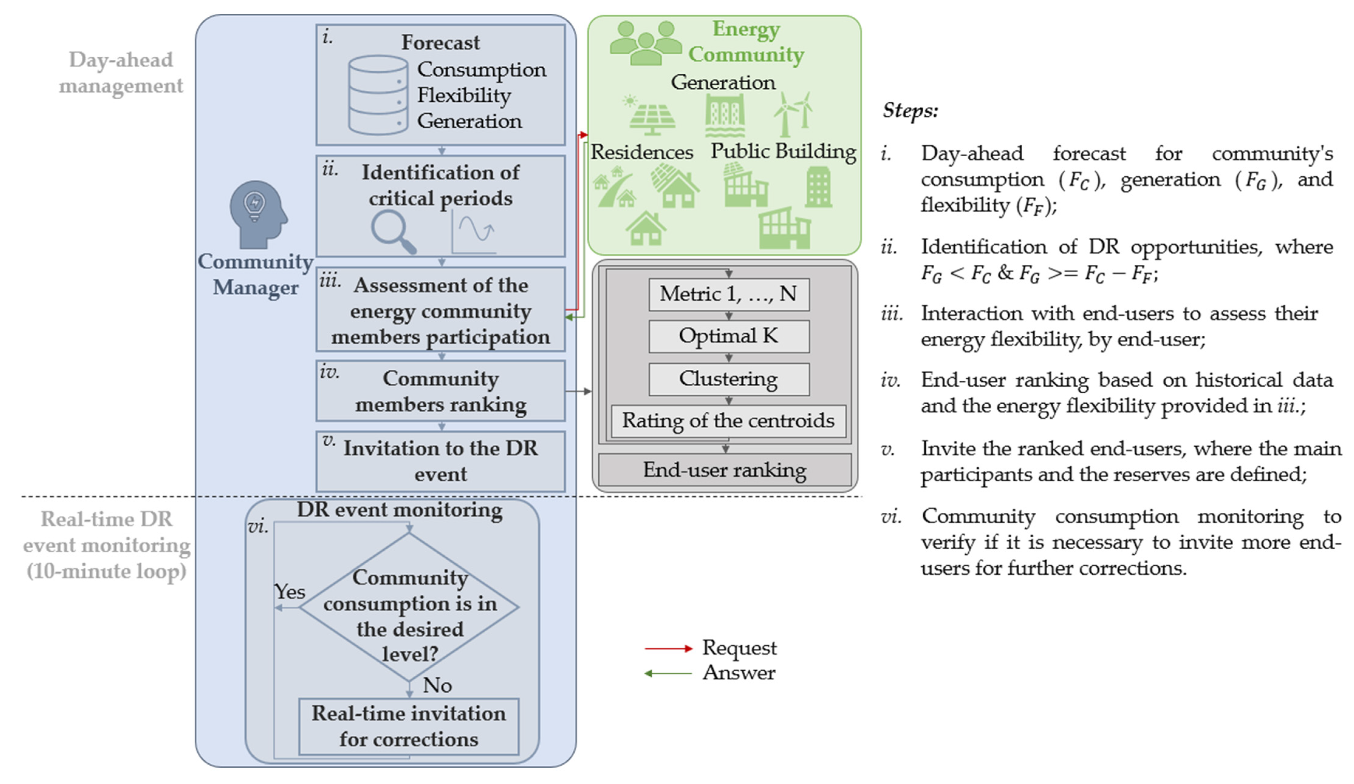
Figure 1 illustrates the six steps of the proposed methodology.
The first step is the day-ahead energy forecasts that enable the perception of the next-day scenario. Then, critical periods where DR programs can be launched to balance the community’s grid are identified. In the next step, end-users are queried regarding their flexibility for the critical periods. Then, considering the flexibility of each end-user and their historical participation data, the community members are classified through clustering algorithms to create a ranking. Next, the invitations for the most suitable end-users are sent after the end-user ranking is calculated. The final step happens during the DR event, where the community energy balance is closely monitored to track the end-users’ participation and to check if the balance is verified.
The proposed methodology is based on an IoT architecture that considers three cooperative entities: the community manager, the end-user, and the respective IoT devices that monitor and control energy loads and resources. Each of these entities can process data; the community manager has the highest level of processing, being responsible for most of the DR event planning.
In this paper, the presented methodology focuses on the end-user ranking to correctly select the ideal end-users who will be invited to participate in the DR programs. In the reviewed literature, none of the studies considered ranking the end-users through the combination of different metrics that evaluate end-user data. Instead, the majority used only the participation history [
11], pattern [
12], or flexibility [
26] to rank the end-users. With this regard, the novelty of the presented methodology is the combination of three metrics to rank end-users, namely the end users’ flexibility, participation ratio, and historic flexibility. The goal of this combination of metrics is to give more opportunities to the end-users to be selected to participate in DR programs.
3.1. Forecast
Initially, the methodology’s first step consists of performing the day-ahead forecast for different data. Forecasting models are essential components to enable energy management ahead of time, aiming to increase efficiency [
27]. Therefore, the use of forecasting models in the literature is common, such as to forecast energy consumption [
28], PV energy generation [
27], wind energy generation [
29], and end-user flexibility for DR participation [
30]. In the scope of this paper, day-ahead energy forecasts for the CEC—namely consumption, PV generation, and flexibility—are performed.
To enable the use and testing of the proposed DR methodology, a forecasting model based on convolutional neural networks (CNN) was conceived, allowing the forecasting of the different data types from the CEC. In the context of this paper, the forecasting algorithms are used as auxiliary tools for the proposed methodology. The forecasting algorithms were tuned using different trials.
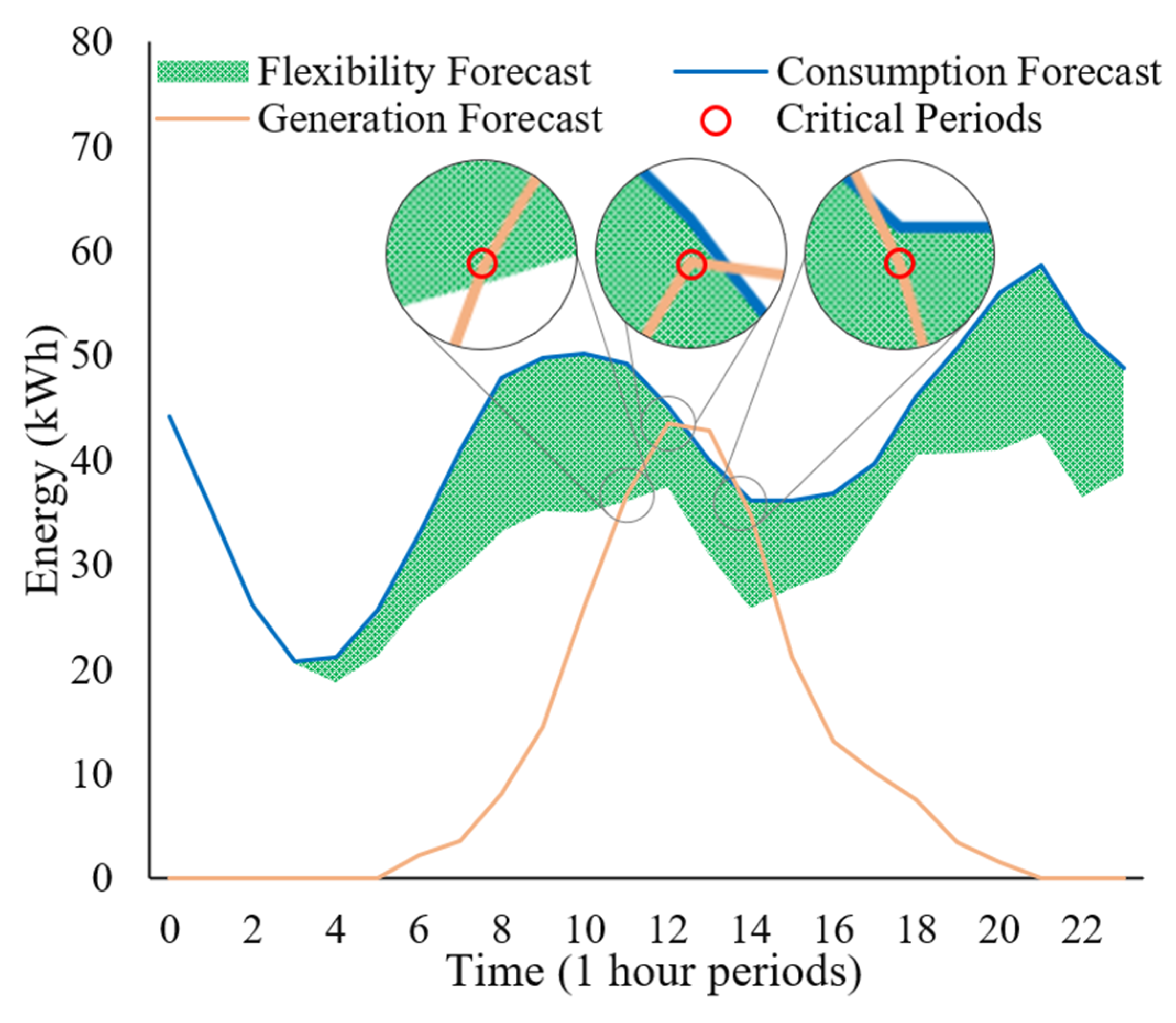
Figure 2 shows the forecasting model’s results, highlighting the forecasted CEC consumption (
), generation (
), and flexibility (
).
The dataset used has one year of historical data (i.e., 8760 records), where each record includes the time frame and respective values of consumption, generation, and flexibility of each end-user. In the case of consumption and flexibility, only working days (i.e., 6288 records) were considered. Each CNN was trained with this dataset, where the data was divided into train (70%), validation (20%), and test (10%).
The CNN model has three layers: the input layer, hidden layer, and output layer. In the case of the day-ahead forecasting model for consumption and flexibility, 17 inputs were considered in the first layer, while 16 were considered for PV generation.
In the forecasting of three CEC data types, these inputs were considered: the respective historical data, 11 lagged variables related to the data type that will be forecasted (t + 1,…, t + 7; t + 25,…, t + 28), and four time-related variables to represent, in two dimensions, the day and year. These four time-related variables represent the time frame in 2D. In addition, in the case of the CEC consumption and flexibility forecast model, the identification of the weekday is also considered as a variable. The hidden layer has 256 neurons and is configured through a rectified linear activation function. The output layer only has one neuron representing the forecasted value related to the data type. To train the CNN algorithm, batches with a size of 32 samples and 30 epochs were considered.
3.2. Identification of Critical Periods
Subsequently, the forecasts are submitted for the community manager’s analysis to determine if critical periods need to be corrected through DR events. Depending on the context, these periods correspond to different situations, such as peak load periods and grid congestion. For example, in the case of peak load periods, it is necessary to perform peak shaving that can be done through demand-side management strategies, technologies that use energy storage systems, and electric vehicles [
31]. In the case of grid congestion, this, occurring more at the distribution and transmission level, can be dealt with by strategies based on energy markets [
32]. Similarly, these periods can also correspond to moments where it is necessary to balance grid resources, that is, to adjust consumption according to the respective generation, and the adjustment needed can be to increase or decrease consumption [
33].
In the context of this paper, the respective critical periods correspond to moments where generation is not sufficient to mitigate consumption, and where the available flexibility could reduce the consumption to an optimum value. In other words, the critical periods are instances where Equations (1) and (2) are verified.
In
Figure 2, the critical periods where energy balancing can be done are identified: at 11:00, at 12:00, and at 14:00. In these periods, the available flexibility allows the reduction of consumption to level off with generation.
3.3. Assessment of the Community Members Participation
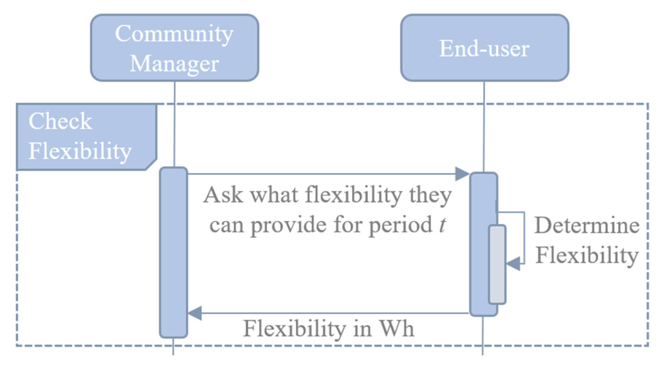
In case there are critical periods, the community manager requests end-users to assess how much flexibility they can provide in the respective periods. This query process is based on the flowchart illustrated in
Figure 3.
The end-users, after the request, calculate how much flexibility they can provide in the respective periods. The flexibility provided by an end-user varies according to the DR model established in the agreement with the community manager, where three possibilities are considered in the proposed methodology. The first possibility is the use of the aggregated flexibility of the residence, where this flexibility only represents the possible reductions in consumption. The second possibility is the use of two types of flexibility, allowing reducible and shiftable loads. Finally, in the third possibility is the use of individual loadsflexibility for each. In the scope of this paper and to facilitate the analysis of the proposed methodology, the end-users will use the first possibility, providing aa aggregated flexibility value. The interaction and communication between the community manager and the end-users is based on the Hypertext Transfer Protocol (HTTP).
3.4. Community Member Ranking
In this step, the community manager makes the ranking of the end-users using unsupervised learning models, like
k-means, to identify which will be the participants for the DR event. This ranking is based on previous studies [
9,
10], where the logic of the ranking and clustering of the end-users participating in DR events is considered.
Figure 1 shows the different processes that occur in this step. The respective ranking takes into account the flexibility that end-users can provide in period
t (obtained in
Section 3.3). It also considers different end-user historical data, namely the total number of times the end-user has participated in DR events, the total number of requests made to the end-user to participate in DR events, the percentage of end-user participation and, finally, the average energy reduction in DR events.
In this way, with the previously mentioned data, metrics can be created, i.e., ways to evaluate end-users, where each metric performs the clustering through two types of data. The two types of data are performing the clustering of end-users considering the percentage of participation and average energy reduction in DR events of each end-user.
The proposed methodology considers the use of three (= 3) metrics: the percentage of participation vs. the average energy reduction, the percentage of participation vs. flexibility for period , and the total number of times the end-user participated vs. the average energy reduction. All end-users are evaluated in each metric , and the combination of the three will result in an end-user ranking table. The silhouette coefficient method is used to find the optimal number of clusters of each metric . Each metric results in clusters, where each one has a centroid of the type (x, y). Each coordinate of the centroid corresponds to the average of the cluster elements for the respective data type.
After performing the metric , it is necessary to apply a points system to them to evaluate the ranking of each of the end-users. In order to make this possible, firstly, in the metric , the evaluation parameter is defined, i.e., the coordinate to which more importance will be given in the analysis of cluster centroids. In this way, the clusters are ordered by evaluation parameter in a decreasing order so the point system in the metric can be subsequently applied. In general, the logic of the proposed point system consists of assigning, per metric, 20 points to the end-users that belong to the best cluster, and the remaining clusters are assigned a score according to their relevance. Thus, if an end-user is always in the best cluster of each metric, it will have points, being the number of metrics under consideration (for this paper, = 3).
Equation (3) shows how the points of cluster
, of a given metric
, are calculated:
where
vpi represents the value of the evaluation parameter of cluster
, i.e., the centroid coordinate of cluster
. In Equation (3),
vpi is divided by the total sum of all (
) clusters’ evaluation parameters to obtain their percentage concerning the other clusters. Then, this percentage is multiplied by 20 to obtain the respective points of the cluster
. It should be noted that the points of an end-user
are the same as the points of the respective cluster to which it belongs.
In each metric
, to assure that the best cluster has a score of 20, Equation (4) is applied, which consists in adding to the score of cluster
the score of the other clusters with fewer points. Considering that the clusters are ordered in descending order, the final points (
) of cluster
is calculated as follows:
Therefore, if we consider the final points of the best cluster (), the calculation would be the points of cluster plus the points of the other remaining clusters ahead (e.g., for , the other clusters will be ). In this way, it is guaranteed that the best cluster has 20 points. For the remaining clusters, the process is the same, except for the last cluster. In the last cluster (), its final points are equal to the points calculated with Equation (3).
After performing the previous processes in the
metrics, it is possible to calculate the score of end-user
, through Equation (5). This equation, considering the scores of the clusters where end-user
was allocated in the
metrics, adds the scores calculated by Equation (4).
For this study, the end-user ranking performed considers two months of historical data, along with the flexibility available for the critical periods.
3.5. Invitation to the Demand Response Event
After the end-user classification, the community manager defines the DR event participants. This way, according to the amount of energy needed for the critical periods, the first-ranked end-users capable of providing the necessary energy reduction are invited as main participants for the DR event. In the scope of this paper, the objective is to achieve a balance in energy consumption and generation at a CEC level. Therefore, not all end-users should be invited to not compromise the balance, as the participation of all end-users could decrease the consumption excessively below the generation.
The end-users that are not invited the day before will be identified as reserves, as they can be invited in real-time during the DR event. It should be highlighted that each end-user has a contract with the respective community manager. In this contract it is defined if the end-user is obliged or not to participate in the DR event, when it is invited to do so, and if the end-user must provide the entirety, or part, of the flexibility. To promote DR event participation, the members of the energy community could use an automation solution for energy management, promoting the use of automated demand response programs where no direct interaction of the user is necessary, after the previous parameterization of the users to define their preferences and restrictions.
DR participation invitations can be made on two occasions. The first, which is always done, consists of sending the invitation at the end of the day before the DR event, which allows the participants to be notified in advance. The second occasion only occurs when the DR event is being monitored. This monitoring is done in a loop every 10 min, where it makes it possible to check whether the DR event is having its effect, i.e., if the community’s consumption has reduced to the desired level. In this way, if the reductions made by the main participants are not enough to reduce the community’s consumption, the reserve participants are invited in real time to assist in the DR event, where further corrections to the CEC consumption are applied.
4. Case Study
The case study used in this paper consists of an energy community with 49 residences and one public building (in this case, a library) equipped with several appliances. The public building and 11 residences have PV generation. In total, the community has a contracted power of 341.55 kVA and an installed power of PV panels of 55.2 kVA. Additionally, the end-users’ consumption and generation are monitored and collected in 15 min periods through IoT devices. In this case study, end-users can opt to participate or not in DR events. In the case that they opt to participate, it is considered that end-users perform reductions equal to the value of the available flexibility.
Table 1 shows the loads available for individual monitoring and control in the community’s end-users. From these loads, seven are considered flexible loads; that is, equipment where consumption can be reduced. The remaining three are loads where consumption cannot be adjusted.
In the scope of this paper, DR events will be launched to balance the community, consisting of requests to end-users to reduce their consumption during critical periods to level the community consumption with the PV generation. This type of DR event considers the aggregated flexibility of each end-user, wherein this way, the confidentiality of the end-user’s load data is maintained.
Figure 2 illustrates the values forecasted by CNN for the community’s consumption, flexibility, and generation that are used as a case study to test the DR methodology. In this figure, it is possible to verify three critical periods at 11:00, 12:00, and 14:00. Of these three critical periods, the periods of 12 and 14 h will be highlighted in the later section, where we intend to balance the community’s electrical grid through the flexibility of the end-users. For example, in the case of the first critical period at 12:00, it is necessary to reduce consumption by around 1.6 kWh, while in the critical period of 14:00, it is necessary to reduce it by 1.4 kWh.
Regarding the classification of end-users, this paper considers three metrics:
Metric 1: the first metric uses the percentage of participation and the average energy reduction, where the evaluation parameter is the percentage of participation;
Metric 2: the second metric considers the total number of times the end-user participated and the average energy reduction, where the evaluation parameter, in this case, is the average energy reduction;
Metric 3: the third metric considers the percentage of participation and flexibility for period , with the respective flexibility being the evaluation parameter.
5. Results
This section illustrates the results obtained from the implementation of the proposed methodology.
Table 2 shows the inputs used to perform the end-user classification through the
k-means algorithm. This table illustrates for each end-user, from left to right, the four historical data considered and the forecasted flexibility in the critical period
. This table shows flexibility corresponding to the critical period of 12:00 as an example. The historical data represent the last two months.
The data in
Table 2 were used to perform the three metrics mentioned in the previous section. It should be noted that end-users with zero flexibility in the critical periods are excluded from the classification, as they cannot contribute to the DR event. As can be seen, five end-users have no flexibility: 9, 28, 32, 36, and 45.
Table 3 demonstrates respective output from the ranking process, illustrating the top 15 end-users that will be invited to the following day’s DR event for 12:00.
Considering the first three end-users, end-users 1, 8, and 12, the data in
Table 2 and
Table 3 show that in metric 1, only end-user 12 obtained the maximum score since they have a higher percentage of participation than the others. End-users 1 and 8 have the same score in this metric because they achieved a similar percentage of participation. In the case of metric 2, only end-user 8 has a maximum score because they have a significantly higher value of the total number of participations. End-users 1 and 12 scored the same despite the values of their average energy reduction being slightly different. This is because they have similar values for the total amount of participation. For metric 3, end-user 1 has the maximum score, while end-users 8 and 12 share a considerably lower score. This difference in scores on this metric is because end-user 1 provides far greater flexibility than end-users 8 and 12.
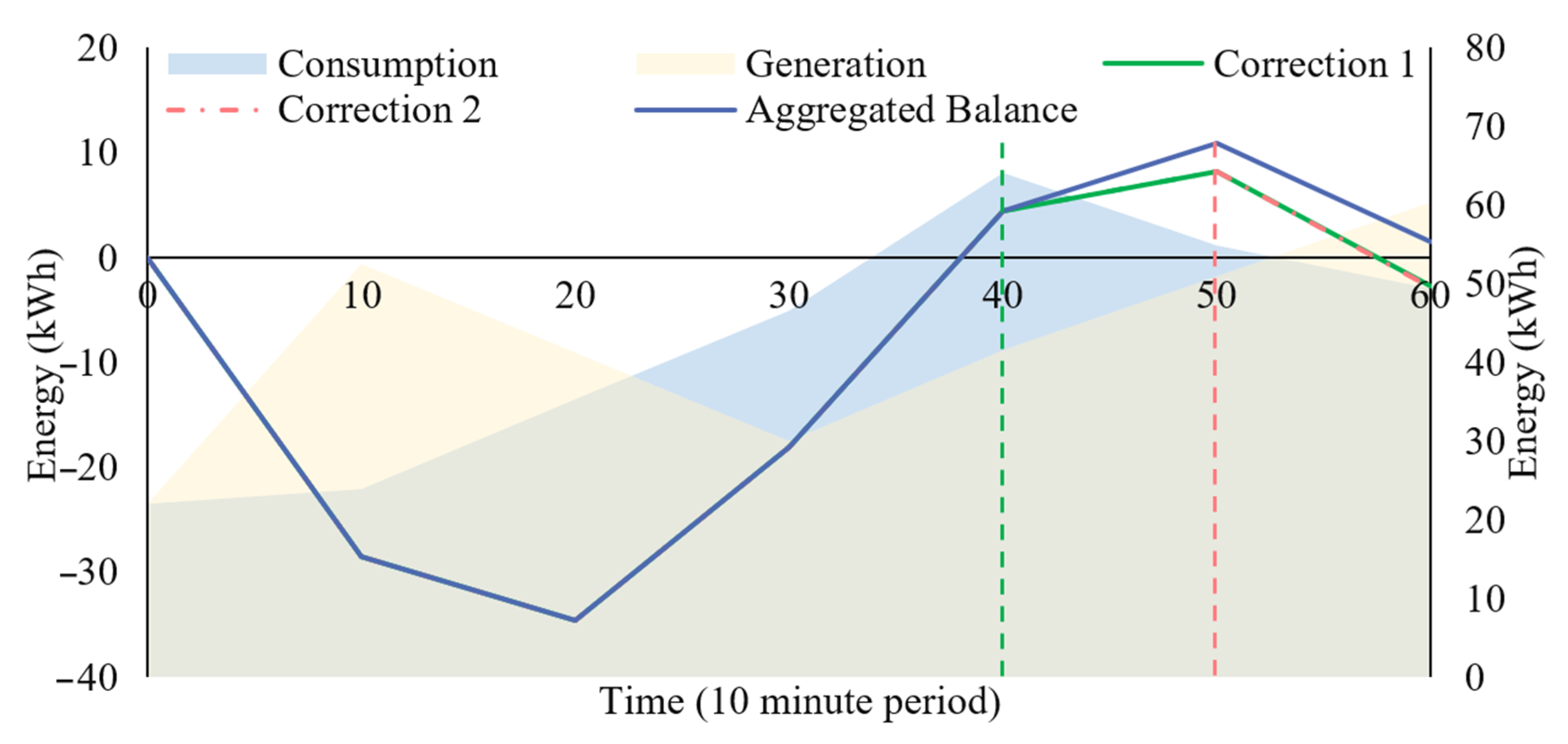
Figure 4 and
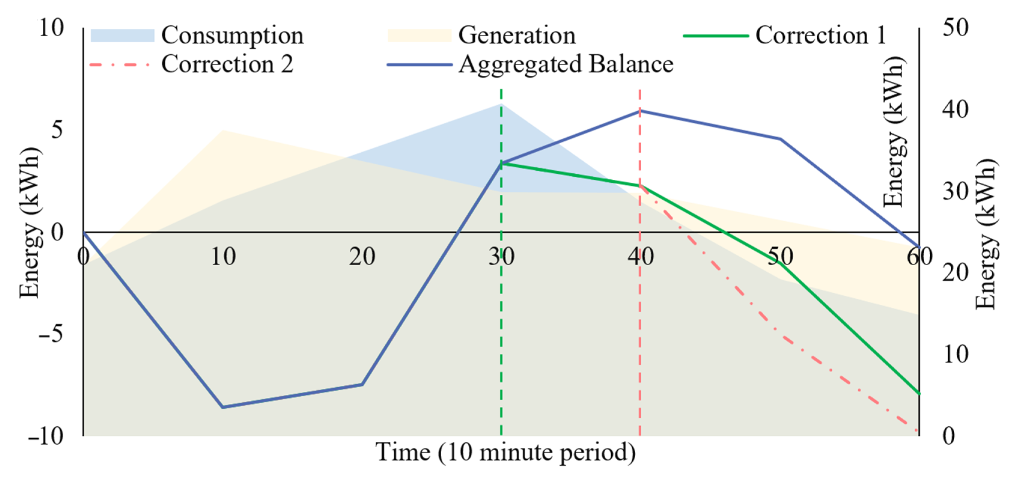
Figure 5 show, respectively, the real-time monitoring performed in a 10-min loop during the DR events that occurred during the critical periods of 12:00 and 14:00.
In each figure, the respective total community energy consumption and PV generation, the aggregated balance, and the respective corrections that were made during the DR event are illustrated. The total community energy consumption shown in the figures already includes the reduction made by the DR participants, i.e., it already includes the flexibility of the invited end-users. In these figures, the vertical axis on the left is for the aggregated balance and corrections (i.e., lines presented on the graph), while the vertical axis on the right is for the total consumption and generation of the community (i.e., areas presented on the graph). The respective aggregated balance corresponds to the aggregation of the community energy balance during the DR event, where the latter represents the total community consumption less the total community PV generation and the flexibility of the participants who were invited for the DR event. It should be noted that the aggregated balance only starts after instant 0, thus ignoring the consumption and generation values existing at that instant. If the DR event successfully balances the community, the last value of the aggregated balance should be close to zero.
The respective corrections are required when the aggregated balance is positive during the DR event. This means that more end-users need to be invited to decrease the overall community consumption. Therefore, these corrections are implemented in periods where the aggregated balance is greater than zero. In these situations, the following X reserve end-users are invited to participate, respecting the ranking positions. The value of X is defined by the sum of end-users’ flexibility that needs to meet with the currently needed reduction (i.e., enough to reduce the aggregated balance).
These corrections are based on the end-users’ flexibilities forecasted on the previous day. Each time a correction is implemented, it is implemented in the period in question and the remaining periods. This adds the flexibility of the reserve end-users chosen for that correction to the main end-users that were invited the day before. If the following period after the first correction turns out not to be enough, another correction is made, where the flexibility of the additional X reserve end-users that were not called in the first correction is used.
It is essential to highlight that the flexibility provided by the end-users during the monitoring of the respective DR events is different from the flexibility forecasted on the previous day. This is the direct result of the forecast errors and end-user participation deviation.
Table 4 presents, for different scenarios, the energy cost and the energy balance in the CEC grid for the two discussed DR events, allowing a deeper analysis of the methodology presented in this paper. In the case where the energy balance is negative (excess of PV generation), it is considered that the energy is sold at a value that represents 50% of the respective dynamic tariff.
The “Independent” scenario represents the case where DR events and the CEC do not exist. In this case, the end-users cannot share their PV generation, and each end-user buys or sells their energy in case of excess PV generation. The “All Flexibility” scenario represents the case where all flexibility provided by end-users is considered in the DR event. This scenario makes it possible to see the maximum reduction obtained with the respective DR event. Finally, the business as usual (“BAU”) scenario represents the case where DR events do not exist, but the concept of CEC exists, allowing the sharing of PV generation among end-users. The “Correction 0” scenario depicts the impact of the participation of the main end-users during the DR event, where in
Figure 4 and
Figure 5 this correction is denominated as the Aggregated Balance. “Correction 1” and “Correction 2” depict the impact of the participation of the reserve end-users during the DR event.
6. Discussion
The results in
Table 3 and
Figure 4 demonstrate that the aggregated balance only considers end-user 1 since their flexibility would be sufficient to mitigate the 1.6 kWh of the predicted excess consumption. From
Figure 4, it can be seen that initially, PV generation is higher than consumption, making the aggregated balance negative. However, 20 min after the event starts, consumption exceeds generation, and the respective aggregated balance becomes positive, with a value of 4.4 kWh at the end of minute 40. In this way, to reduce the aggregated balance to zero or a value close to it, Correction 1 is applied at minute 40, which considers the flexibility foreseen on the previous day of 38 end-users. These end-users are the ones who succeed the first ranked end-user, where in total it was predicted to provide about 4.4 kWh of flexibility during the DR event.
The application of Correction 1 was not enough, and, at minute 50, Correction 2 was applied. This second Correction considers the forecasted flexibility of the six remaining end-users, which is equal to 0.62 kWh. As shown in
Figure 4, Correction 2 had little impact due to the little flexibility remaining.
In the period of 12:00, at the end of this DR event, and only considering end-user 1 participation (i.e., the blue line in
Figure 4), it is possible to verify that the aggregated balance would be positive, that is, it was not enough to handle the respective critical period. Thus, with the continuous monitoring of the DR event every 10 min, it was possible to make the necessary corrections. At the end of the event, Corrections 1 and 2 (dashed red line in
Figure 4) reduced the aggregated balance to a negative value, thus dealing with the critical 12:00 period. Furthermore, at the end of this event, total PV generation exceeded the value of total community consumption, further contributing to the reduction in the value of the aggregated balance.
In the case of
Figure 5, the aggregated balance also only considers the flexibility of end-user 1. This is due to the forecasted flexibility on the previous day for this end-user being 4.4 kWh, which is more than enough for the 1.4 kWh of excess consumption. In this case, it is also seen that at the beginning of the DR event, there is an excess of PV generation. However, this only occurs until minute 20. Thereafter, between minutes 20 and 30, the total consumption of the community exceeds the total PV generation, causing the value of the aggregated balance to increase such that, at minute 30, the aggregated balance become positive. Thus, Correction 1 is applied where it was necessary to use the flexibility of the eight subsequent end-users to attenuate the value of the aggregated balance equal to 3.36 kWh. As shown in
Figure 5, when comparing the aggregated balance with and without Correction 1 (i.e., lines blue and green in
Figure 5), it can be seen that the reduction made was significant. However, the value is still positive at minute 40. Thus, Correction 2 is applied on top of Correction 1. In this case, an additional 11 end-users were invited to participate at minute 40, where they were expected to be able to provide, in total, 2.26 kWh of flexibility. As can be seen at minute 50 (dashed red line in
Figure 5), both corrections caused the aggregated balance value to become negative, with Correction 2 reaching a significantly higher reduction than expected.
In the period at 14:00, at the end of the DR event, the aggregated balance that only considers the flexibility provided by end-user 1 would be enough to mitigate the critical period (represented by the blue line in
Figure 5). However, corrections were still made since it is difficult to know how the aggregated balance will behave during the DR event. In this case, the corrections made would not be necessary at the end of the DR event.
Considering the monitoring done in both DR events, it can be seen that end-users provided more flexibility during the critical period of 14:00. A possible explanation for this is that the critical period of 12:00 comprises the lunchtime of most end-users. Thus, there is not much flexibility for each end-user, which consequently causes several end-users to be called to participate during the respective DR event.
Regarding the energy values illustrated in
Table 4, these correspond to the real data of the CEC during the hours of the DR events, where these diverge from the forecasted values.
Through the comparison of the scenarios presented in this table, the economic benefits can be highlighted. Comparing the Independent and BAU scenarios, it is possible to verify the economic benefits obtained considering the CEC concept, where the benefits are approximately EUR 2.2 in the first DR event and EUR 1.33 in the second. With the All Flexibility scenario, the maximum energy reduction can be made, wherein at the end of both DR events, there is excess generation. Comparing this scenario with the BAU scenario, it can be seen that the profits of using all the flexibility provided by the end-users are about EUR 0.52 in the first event and EUR 1.1 in the second. Finally, comparing the BAU and Correction 2 scenarios, the economic benefits obtained with the DR events are verified, where in the first event they are EUR 0.42, and in the second they are EUR 0.89. With these two DR events, the total economic benefits are EUR 1.31.
Although achieving promising results, this study is susceptible to improvements. A future improvement is the consideration of shifting flexibility and the respective new metric to assess it. In this way, the DR model is less limited and enables better use of PV generation. Furthermore, to increase the efficiency of DR event monitoring, one other possible improvement is the implementation of a 10-minute-ahead forecast algorithm for the CEC’s energy resources.


