
Experimental Study on Connection Characteristics of Rough Fractures Induced by Multi-Stage Hydraulic Fracturing in Tight Reservoirs


Abstract
:1. Introduction
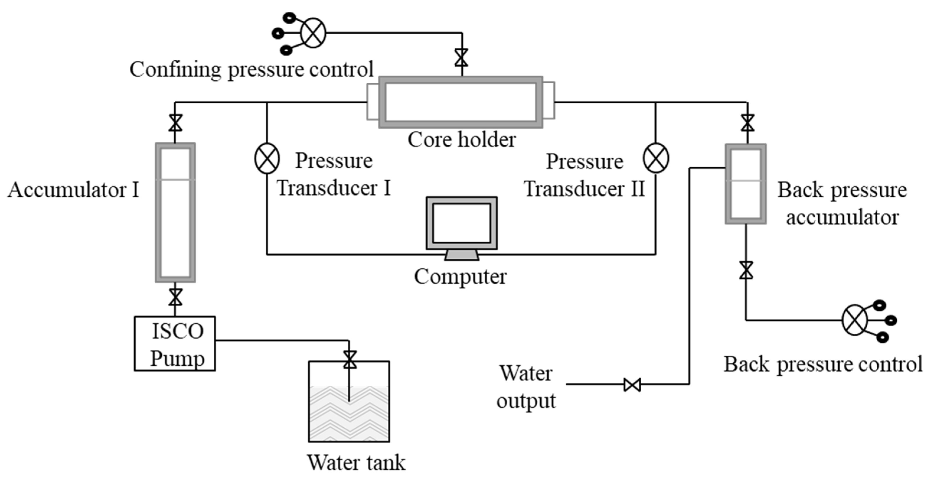
2. Experimental Sections
2.1. Experiment Materials
2.2. Experiment Method
3. Results
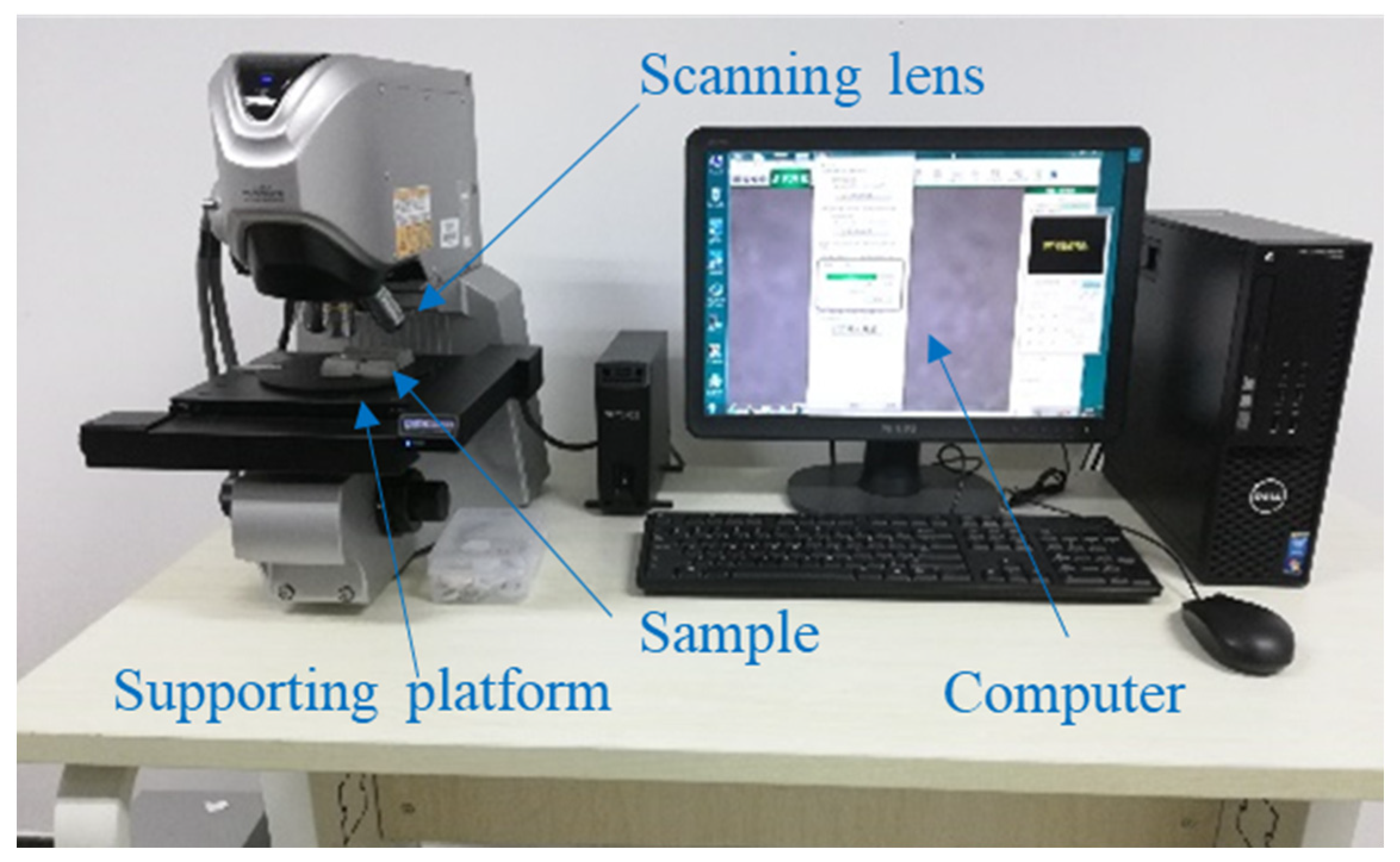
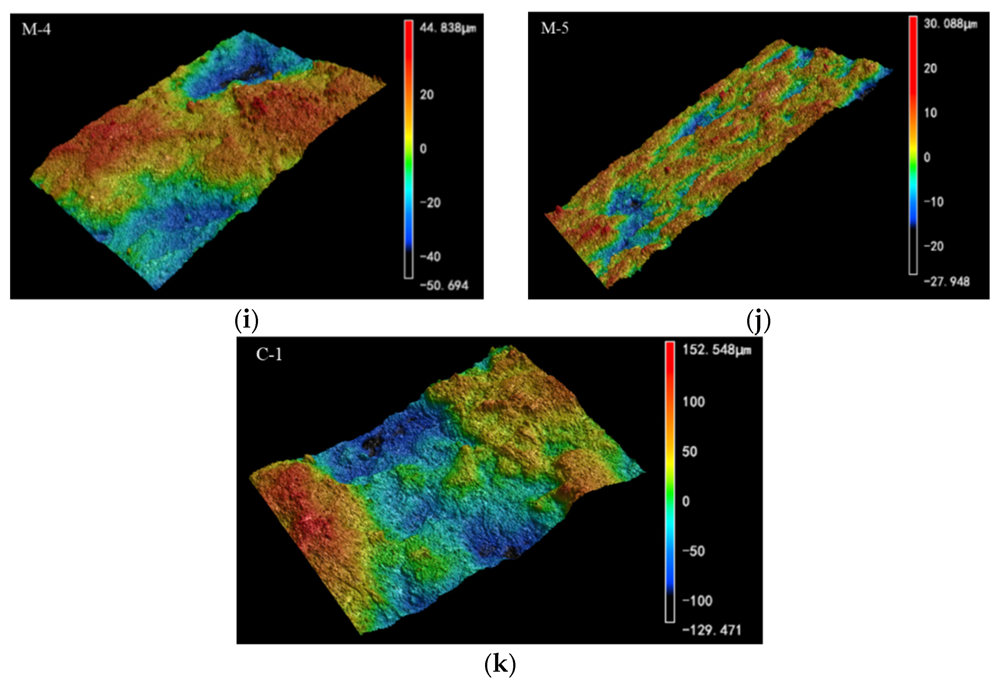
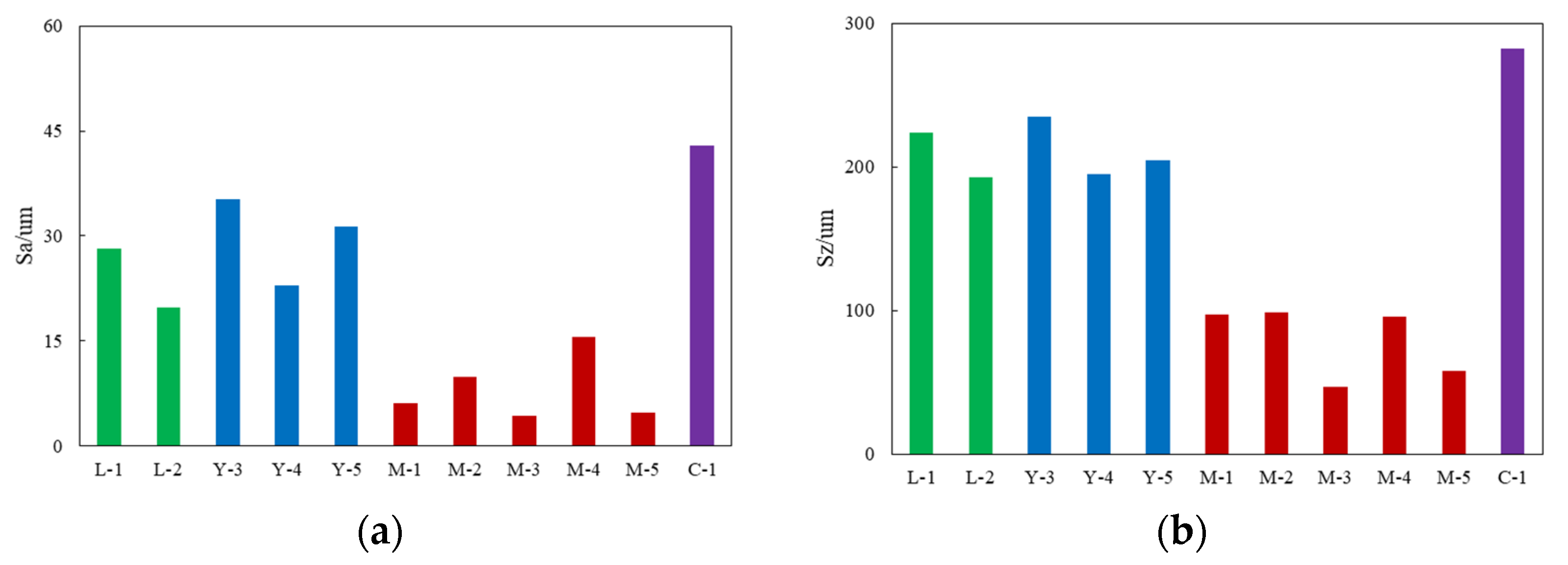
3.1. The Roughness of Fracture Surface
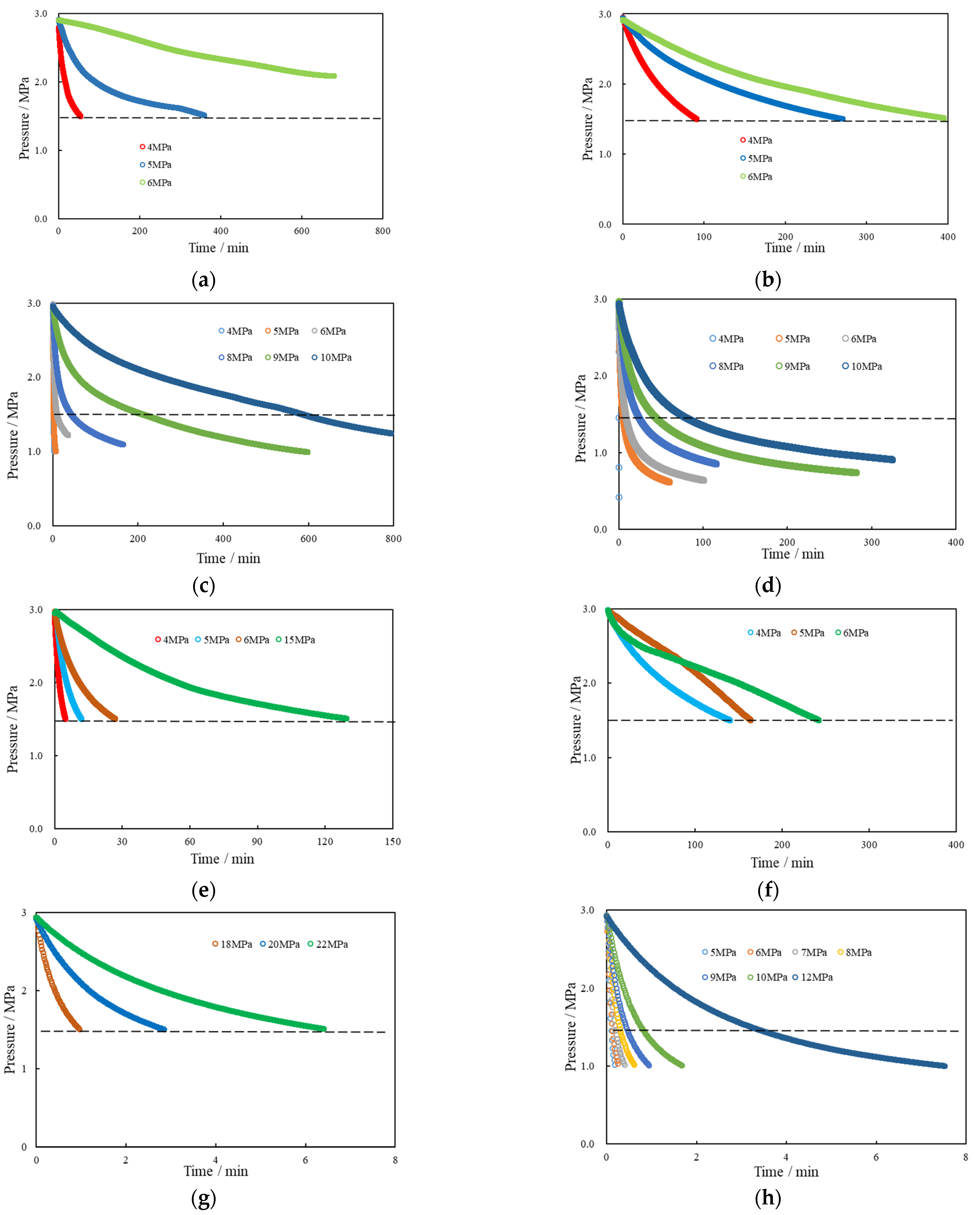
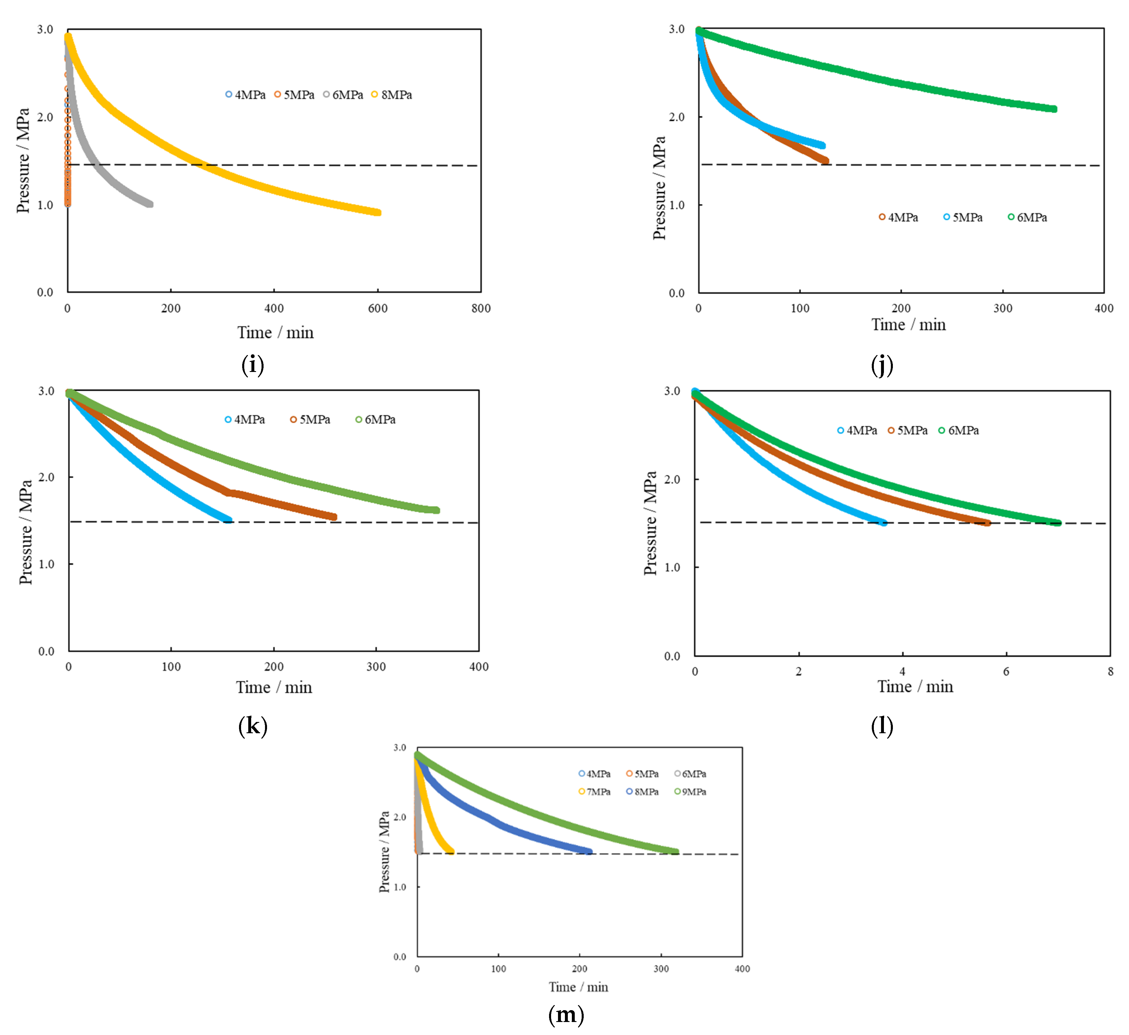
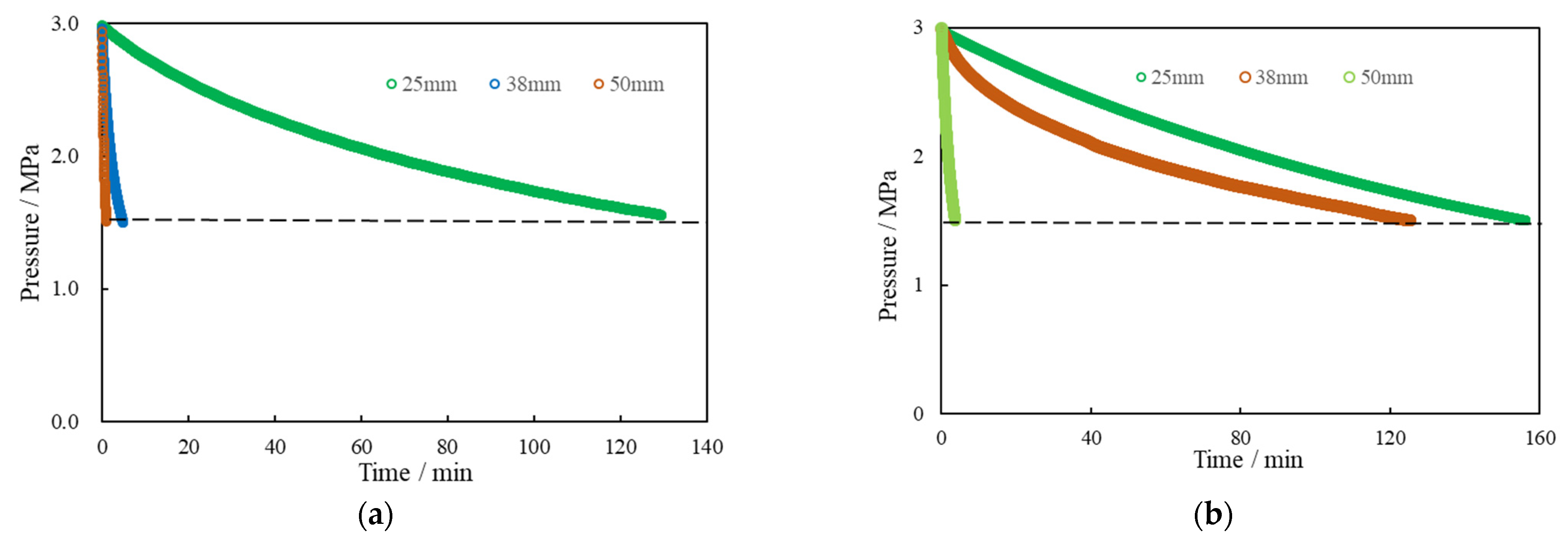
3.2. The Characteristics of Pressure Evolution
3.3. The Factors Influencing Fracture Connection
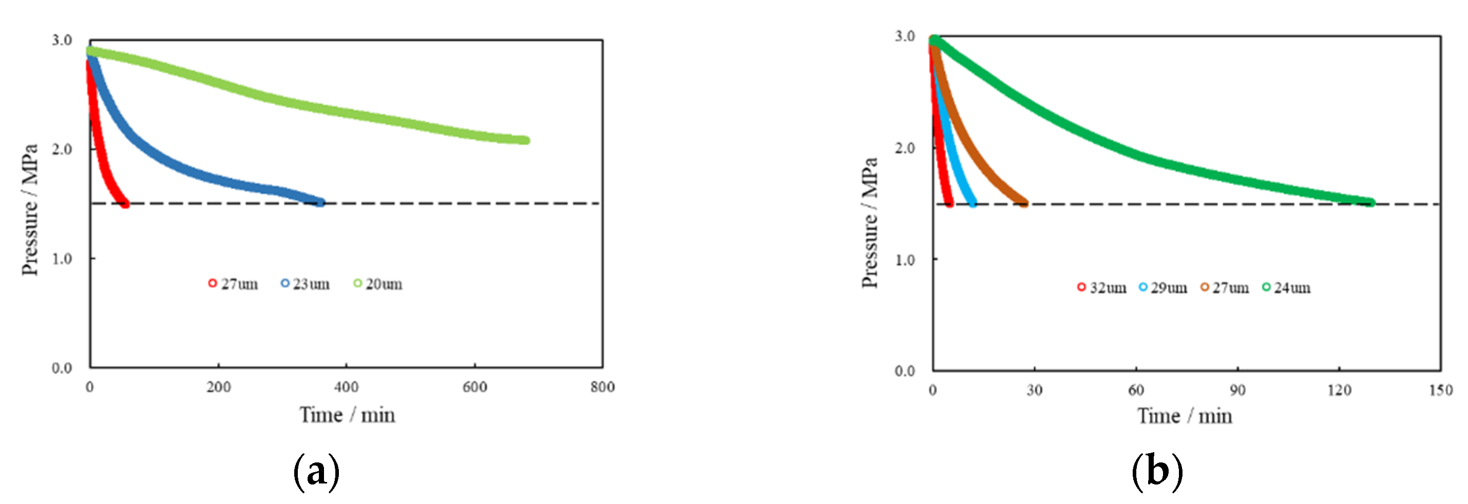
3.3.1. Fracture Aperture
3.3.2. Fracture Roughness
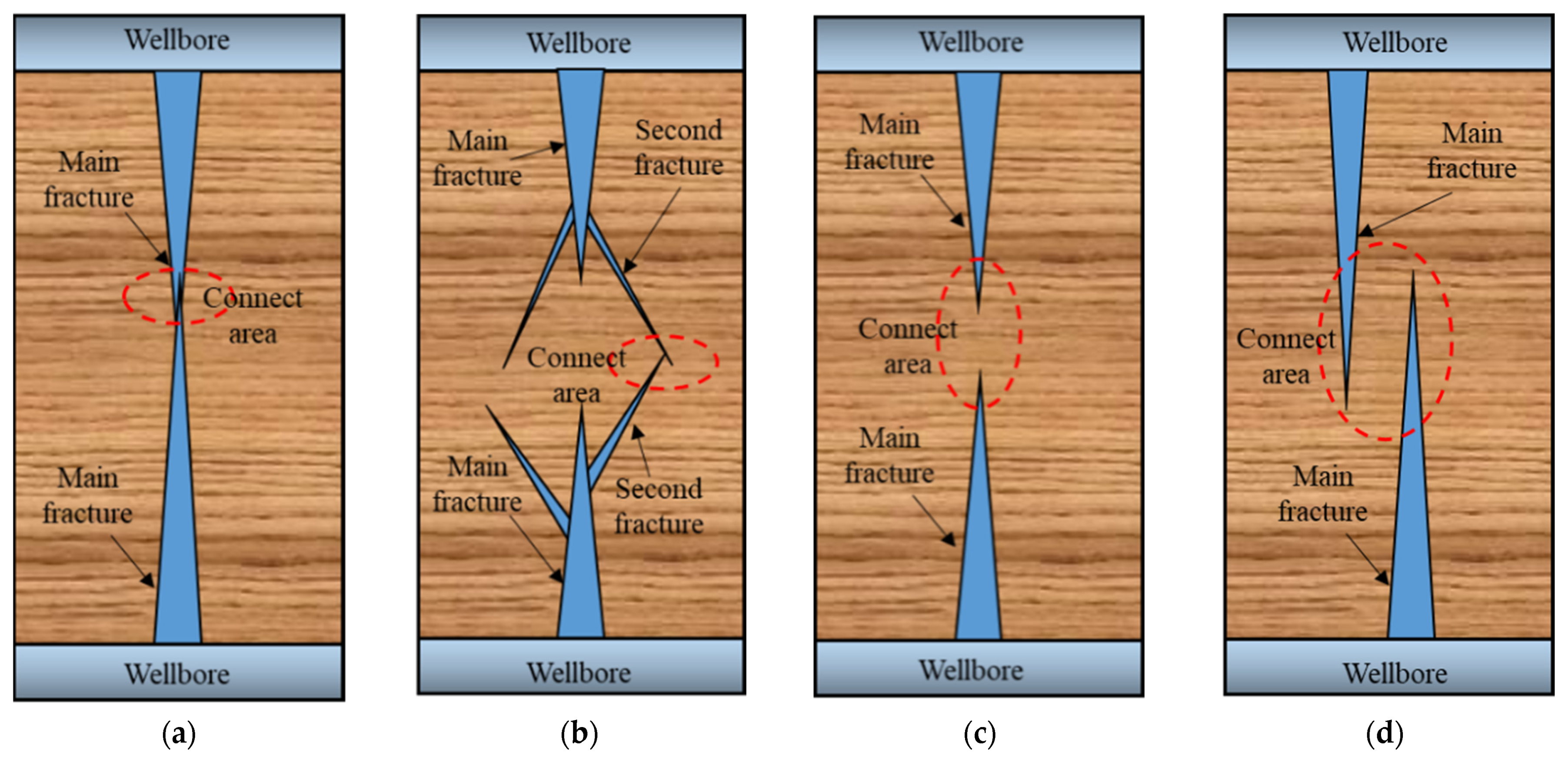
3.3.3. The Contact Area
3.3.4. The Property of Fracturing Fluid
4. Discussion
4.1. The Effect of Scale and Time
4.2. Application of Interwell-Fracturing Interference
4.3. The Limitations of This Study
5. Conclusions
- (1)
- As an important mechanism of interwell interference, fracture connectivity has a strong scale effect and time effect. If larger areas of fractures are formed during fracturing, it will lead to a longer-term impact on production, which is shown as a strong scale effect. After entering the reservoirs, the fracturing fluid is easy to interact with the fracture surface of samples with a relatively high content of swelling clay minerals. With the increase in time, the fracture surface is damaged and the fracture connectivity decreases, which shows a strong time effect;
- (2)
- Fracture connectivity is related to the fracture aperture, the roughness of the fracture surface, the fracture closure contact area, and the viscosity of a fracturing fluid. The decrease in fracture aperture and the increase in the fluid viscosity leads to a significant reduction in fracture connectivity, while higher fracture surface roughness and larger contact area can make fracture connectivity better;
- (3)
- The connectivity of rough fractures is characterized by half-decayed pressure and a laboratory evaluation method for fracture connectivity is established. The fracture connectivity evaluated based on the calculated half-life time is consistent with the experimental results. The total time of the interwell interference can be calculated with the fracture interference time and the matrix interference time. It is equal to the sum of the time for the pressure to pass through both the fracture and the matrix.
Author Contributions
Funding
Institutional Review Board Statement
Informed Consent Statement
Data Availability Statement
Conflicts of Interest
References
- Khanal, A.; Weijermars, R. Distinguishing Fracture Conductivity and Fracture Flux: A Systematic Investigation of Individual Fracture Contribution to Well Productivity. In Proceedings of the Unconventional Resources Technology Conference, Virtual, 20–22 July 2020. [Google Scholar] [CrossRef]
- Zheng, P.; Xia, Y.; Yao, T.; Jiang, X.; Xiao, P.; He, Z.; Zhou, D. Formation mechanisms of hydraulic fracture network based on fracture interaction. Energy 2022, 243, 123057. [Google Scholar] [CrossRef]
- Khanal, A.; Weijermars, R. Pressure depletion and drained rock volume near hydraulically fractured parent and child wells. J. Pet. Sci. Eng. 2019, 172, 607–626. [Google Scholar] [CrossRef]
- Yaich, E.; Diaz De Souza, O.C.; Foster, R.A.; Abou-sayed, I.S. A Methodology to Quantify the Impact of Well Interference and Optimize Well Spacing in the Marcellus Shale. In Proceedings of the SPE/CSUR Unconventional Resources Conference, Calgary, AB, Canada, 20 October 2015. [Google Scholar] [CrossRef]
- Iino, A.; Jung, H.Y.; Onishi, T.; Datta-Gupta, A. Rapid Simulation Accounting for Well Interference in Unconventional Reservoirs Using Fast Marching Method. In Proceedings of the SPE/AAPG/SEG Unconventional Resources Technology Conference, Virtual, 20–22 July 2020. [Google Scholar] [CrossRef]
- Al-Rbeawi, S. An approach for the performance-impact of parent-child wellbores spacing and hydraulic fractures cluster spacing in conventional and unconventional reservoirs—ScienceDirect. J. Pet. Ence Eng. 2020, 185, 106570. [Google Scholar] [CrossRef]
- Manchanda, R.; Bhardwaj, P.; Hwang, J.; Sharma, M.M. Parent-Child Fracture Interference: Explanation and Mitigation of Child Well Underperformance. In Proceedings of the SPE Hydraulic Fracturing Technology Conference and Exhibition, The Woodlands, TX, USA, 23–25 January 2018. [Google Scholar] [CrossRef]
- Ajani, A.A.; Kelkar, M.G. Interference Study in Shale Plays. In Proceedings of the SPE Hydraulic Fracturing Technology Conference, Woodlands, TX, USA, 6–8 February 2012. [Google Scholar]
- Lawal, H.; Abolo, N.; Jackson, G.; Sahai, V.; Flores, C.P. A Quantitative Approach to Analyze Fracture Area Loss in Shale Gas Reservoirs. In Proceedings of the SPE Latin America and Caribbean Petroleum Engineering Conference, Maracaibo, Venezuela, 21–23 May 2014. [Google Scholar]
- Tang, H.; Chai, Z.; Yan, B.; Killough, J. Application of Multi-segment Well Modeling to Simulate Well Interference. In Proceedings of the SPE/AAPG/SEG Unconventional Resources Technology Conference, Austin, TX, USA, 24–26 July 2017. [Google Scholar]
- George, E.K.; Michael, F.R.; Cory, S. Frac Hit Induced Production Losses: Evaluating Root Causes, Damage Location, Possible Prevention Methods and Success of Remedial Treatments. In Proceedings of the SPE Annual Technical Conference and Exhibition, San Antonio, TX, USA, 9–11 October 2017. [Google Scholar]
- Esquivel, R.; Blasingame, T.A. Optimizing the Development of the Haynesville Shale-Lessons-Learned from Well-to-Well Hydraulic Fracture Interference. In Proceedings of the SPE Unconventional Resources Technology Conference, Austin, TX, USA, 24–26 July 2017. [Google Scholar]
- Sun, H.; Zhou, D.; Chawathe, A.; Liang, B. Understanding the Frac-Hits Impact on a Midland Basin Tight-Oil Well Production. In Proceedings of the Unconventional Resources Technology Conference, Austin, TX, USA, 24–26 July 2017. [Google Scholar] [CrossRef]
- Jacobs, T. Frac Hits Reveal Well Spacing May be Too Tight, Completion Volumes Too Large. J. Pet. Technol. 2017, 69, 35–38. [Google Scholar] [CrossRef]
- Anusarn, S.; Li, J.; Wu, K.; Wang, Y.; Shi, X.; Yin, C.; Li, Y. Fracture Hits Analysis for Parent-Child Well Development. In Proceedings of the 53rd US Rock Mechanics/Geomechanics Symposium, New York City, NY, USA, 23–26 June 2019. [Google Scholar]
- Morales, A.; Zhang, K.; Gakhar, K.; Marongiu Porcu, M.; Lee, D.; Shan, D.; Acock, A. Advanced Modeling of Interwell Fracturing Interference: An Eagle Ford Shale Oil Study—Refracturing. In Proceedings of the SPE Hydraulic Fracturing Technology Conference, The Woodlands, TX, USA, 9–11 February 2016. [Google Scholar] [CrossRef]
- Xu, L.; Ogle, J.; Collier, T. Fracture Hit Mitigation through Surfactant-Based Treatment Fluids in Parent Wells. In Proceedings of the SPE Liquids-Rich Basins Conference—North America, Odessa, TX, USA, 7–8 November 2019. [Google Scholar] [CrossRef]
- Luo, S.; Zhao, Z.; Peng, H.; Pu, H. The role of fracture surface roughness in macroscopic fluid flow and heat transfer in fractured rocks. Int. J. Rock Mech. Min. Sci. 2016, 87, 29–38. [Google Scholar] [CrossRef]
- Rossen, W.R.; Gu, Y.; Lake, L.W. Connectivity and Permeability in Fracture Networks Obeying Power-Law Statistics. In Proceedings of the SPE Permian Basin Oil and Gas Recovery Conference, Midland, TX, USA, 21–23 March 2000. [Google Scholar] [CrossRef]
- Li, J.; Liu, Y.; Huang, C. Multi-stage fracturing horizontal well interference test model and its application. Lithol. Reserv. 2018, 30, 138–144. [Google Scholar]
- Awada, A.; Santo, M.; Lougheed, D.; Xu, D.; Virues, C. Is That Interference? A Work Flow for Identifying and Analyzing Communication through Hydraulic Fractures in a Multiwell Pad. SPE J. 2016, 21, 1554–1566. [Google Scholar] [CrossRef]
- Haghshenas, B.; Qanbari, F. Quantitative Analysis of Inter-Well Communication in Tight Reservoirs: Examples from Montney Formation. In Proceedings of the SPE Canada Unconventional Resources Conference, Virtual, 28 September–2 October 2020. [Google Scholar] [CrossRef]
- Felisa, G.; Lenci, A.; Lauriola, I.; Longo, S.; Di Federico, V. Flow of truncated power-law fluid in fracture channels of variable aperture. Adv. Water Resour. 2018, 122, 317–327. [Google Scholar] [CrossRef]
- Wang, J.; Zhao, W.; Liu, H.; Liu, F.; Zhang, T.; Dou, L.; Yang, X.; Li, B. Inter-well interferences and their influencing factors during water flooding in fractured-vuggy carbonate reservoirs. Pet. Explor. Dev. 2020, 47, 1062–1073. [Google Scholar] [CrossRef]
- Daneshy, A. Analysis of Horizontal Well Fracture Interactions, and Completion Steps for Reducing the Resulting Production Interference. In Proceedings of the SPE Annual Technical Conference and Exhibition, Dallas, TX, USA, 24–26 September 2018. [Google Scholar] [CrossRef]
- Wang, M.; Chen, Y.F.; Ma, G.W.; Zhou, J.Q.; Zhou, C.B. Influence of surface roughness on nonlinear flow behaviors in 3D self-affine rough fractures: Lattice Boltzmann simulations. Adv. Water Resour. 2016, 96, 373–388. [Google Scholar] [CrossRef]
- Rong, G.; Yang, J.; Cheng, L.; Zhou, C. Laboratory investigation of nonlinear flow characteristics in rough fractures during shear process. J. Hydrol. 2016, 541, 1385–1394. [Google Scholar] [CrossRef]
- Babadagli, T.; Ren, X.; Develi, K. Effects of fractal surface roughness and lithology on single and multiphase flow in a single fracture: An experimental investigation. Int. J. Multiph. Flow 2015, 68, 40–58. [Google Scholar] [CrossRef]
- Zou, L.; Jing, L.; Cvetkovic, V. Effects of Sorption on Solute Transport in a Single Rough Rock Fracture. In Proceedings of the 13th International Congress on Rock Mechanics (ISRM Congress 2015), Montréal, QC, Canada, 9–14 May 2015. [Google Scholar]
- Lee, H.B.; Yeo, I.W.; Lee, K.K. The modified Reynolds equation for non-wetting fluid flow through a rough-walled rock fracture. Adv. Water Resour. 2013, 53, 242–249. [Google Scholar] [CrossRef]
- Crandall, D.; Bromhal, G.; Karpyn, Z.T. Numerical simulations examining the relationship between wall-roughness and fluid flow in rock fractures. Int. J. Rock Mech. Min. Sci. 2010, 47, 784–796. [Google Scholar] [CrossRef]
- Zhou, T.; Zhang, S.; Yang, L.; Ma, X.; Zou, Y.; Lin, H. Experimental investigation on fracture surface strength softening induced by fracturing fluid imbibition and its impacts on flow conductivity in shale reservoirs. J. Nat. Gas Sci. Eng. 2016, 36, 893–905. [Google Scholar] [CrossRef]
- Wang, X.; Chen, Z. Hydrodynamic analysis of rock permeability test by transient method. Chin. J. Rock Mech. Eng. 2006, 25, 3098–3103. [Google Scholar]


| Number | Basin | Formation | Lithology | Depth/m |
|---|---|---|---|---|
| L | the Junggar Basin | the Lucaogou Formation | Shale | 2850 |
| Y | the Ordos Basin | the Yanchang Formation | Tight sandstone | 1875 |
| M | the Sichuan Basin | the Longmaxi Formation | Shale | 2520 |
| C | the Songliao Basin | the Yingcheng Formation | tight volcanic rock | 2470 |
| Number | Mineral Content/% | Clay Mineral Content/% | |||||||||
|---|---|---|---|---|---|---|---|---|---|---|---|
| Quartz | Feldspar | Calcite | Dolomite | Iron Ore | Clay Mineral | Illite | Montmorillonite | Illite/Smectite Mixed Layer | Chlorite | Kaolinite | |
| L | 23.7 | 56.5 | 0.0 | 13.1 | 0.0 | 6.7 | 21.0 | 0.0 | 0.0 | 55.0 | 24.0 |
| Y | 70.5 | 9.2 | 1.6 | 3.9 | 0.0 | 14.8 | 33.0 | 0.0 | 43.0 | 20.0 | 4.0 |
| M | 40.3 | 8.8 | 7.5 | 6.5 | 0 | 36.9 | 15.9 | 4.3 | 62.3 | 8.7 | 8.8 |
| C | 36.8 | 48.8 | 6.0 | 0.0 | 0.0 | 8.4 | 14.0 | 0.0 | 44.0 | 42.0 | 0.0 |
| Serial Number | Diameter/cm | Length/cm | Permeability/mD | Porosity/% | Liquid Types |
|---|---|---|---|---|---|
| L-1 | 2.5 | 5.0 | 0.0012 | 7.2 | Distilled water |
| L-2 | 2.5 | 5.0 | 0.0018 | 6.8 | Distilled water/Slick water |
| Y-1 | 2.5 | 5.0 | 0.011 | 13.1 | distilled water |
| Y-2 | 2.5 | 10.0 | 0.025 | 12.7 | Distilled water/Slick water |
| Y-3 | 2.5 | 5.0 | 0.017 | 15.3 | Distilled water |
| Y-4 | 3.8 | 5.0 | 0.016 | 13.9 | Distilled water |
| Y-5 | 5.0 | 5.0 | 0.022 | 14.5 | Distilled water |
| M-1 | 2.5 | 5.0 | 0.0011 | 3.2 | Distilled water |
| M-2 | 2.5 | 5.0 | 0.0018 | 5.1 | Distilled water |
| M-3 | 2.5 | 5.0 | 0.0032 | 4.9 | Distilled water |
| M-4 | 3.8 | 5.0 | 0.0025 | 5.7 | Distilled water |
| M-5 | 5.0 | 5.0 | 0.0021 | 4.1 | Distilled water |
| C-1 | 2.5 | 5.0 | 0.0072 | 10.2 | Distilled water |
| C-2 | 2.5 | 5.0 | 0.0081 | 9.7 | Distilled water |
| C-3 | 2.5 | 5.0 | 0.0055 | 8.6 | Distilled water |
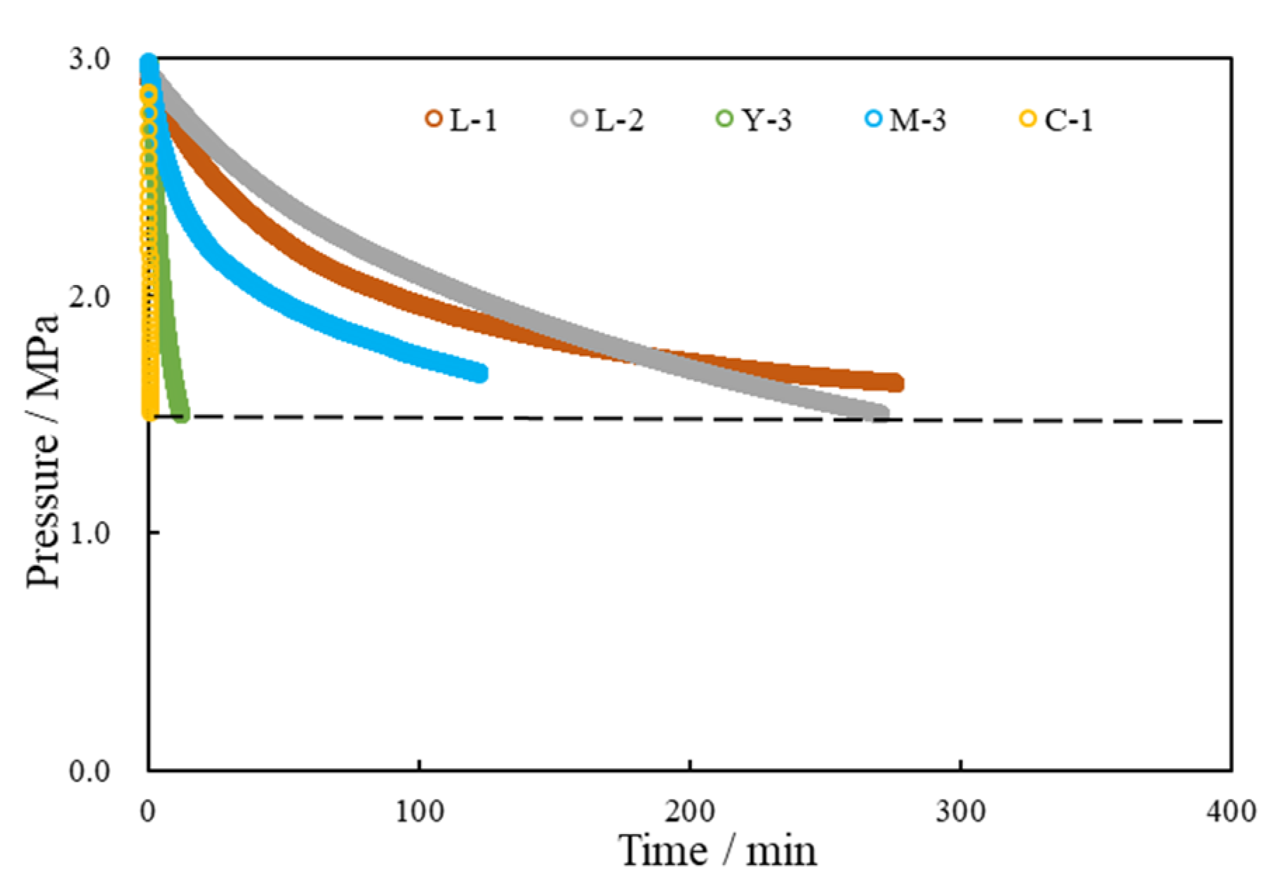
| Number | Flow Rate/(mL/min) | Injection Pressure/MPa | Outlet Pressure/MPa | Liquid Type | Half-Life Time/min |
|---|---|---|---|---|---|
| L-1 | 0.0035 | 3 | 1 | distilled water | 230 |
| L-2 | 0.04 | 3 | 1 | distilled water | 220 |
| Y-3 | 0.5 | 3 | 1 | distilled water | 15 |
| M-3 | 0.08 | 3 | 1 | distilled water | 110 |
| C-1 | 0.3 | 3 | 1 | distilled water | 20 |
Publisher’s Note: MDPI stays neutral with regard to jurisdictional claims in published maps and institutional affiliations. |
© 2022 by the authors. Licensee MDPI, Basel, Switzerland. This article is an open access article distributed under the terms and conditions of the Creative Commons Attribution (CC BY) license (https://creativecommons.org/licenses/by/4.0/).
Share and Cite
Zhang, Y.; Yan, L.; Ge, H.; Liu, S.; Zhou, D. Experimental Study on Connection Characteristics of Rough Fractures Induced by Multi-Stage Hydraulic Fracturing in Tight Reservoirs. Energies 2022, 15, 2377. https://doi.org/10.3390/en15072377
Zhang Y, Yan L, Ge H, Liu S, Zhou D. Experimental Study on Connection Characteristics of Rough Fractures Induced by Multi-Stage Hydraulic Fracturing in Tight Reservoirs. Energies. 2022; 15(7):2377. https://doi.org/10.3390/en15072377
Chicago/Turabian StyleZhang, Yanjun, Le Yan, Hongkui Ge, Shun Liu, and Desheng Zhou. 2022. "Experimental Study on Connection Characteristics of Rough Fractures Induced by Multi-Stage Hydraulic Fracturing in Tight Reservoirs" Energies 15, no. 7: 2377. https://doi.org/10.3390/en15072377
APA StyleZhang, Y., Yan, L., Ge, H., Liu, S., & Zhou, D. (2022). Experimental Study on Connection Characteristics of Rough Fractures Induced by Multi-Stage Hydraulic Fracturing in Tight Reservoirs. Energies, 15(7), 2377. https://doi.org/10.3390/en15072377