Operational Emissions in Prosuming Dwellings: A Study Comparing Different Sources of Grid CO₂ Intensity Values in South Wales, UK ^†

Abstract

This paper analysed operational CO₂ emissions from electricity grid interaction in photovoltaic prosumer dwellings in South Wales, UK. Operational CO₂ emissions were quantified in four prosumer dwellings aiming to analyse (1) the differences in the result when time-varying data and static emission factors are used, and (2) the association of load-matching indicators to the results. Electricity balance data were obtained through monitoring (April 2020 to March 2021), and three sources for the grid’s CO₂ intensity were considered: (1) UK nationwide average time-varying values (UK), (2) South Wales (SW) average time-varying values and (3) the UK Government’s official CO₂ emissions factor (EF) for the study period. UK and SW grid CO₂ intensity were obtained as dynamic data flows in a 30 min resolution, whereas EF was a year constant. Gross CO₂ emissions calculated using SW data reached the highest emissions results: between 67.5% and 69.3% higher than the results obtained using the UK time-varying data, and between 41.1% and 45.1% higher than using the EF. The differences between the obtained yearly net emissions using dynamic data and the EF in each studied dwelling ranged between 6.2% and 294%. Results also show that the definition of geographic boundaries for location-based approach calculations can significantly affect the obtained emissions values.

1. Introduction

Residential buildings were reported to account for 22% of worldwide final energy use and 17% of all emissions in 2021 [1]. Along with several other measures to reduce these figures, the International Energy Agency (IEA) has highlighted that in order to reach a net zero emissions scenario by 2050, an average annual photovoltaic (PV) generation growth of 24% is expected worldwide [2]. Due to substantial decreases in production and installation costs [3], on-grid PV panel systems have become a mainstream measure to reduce operational CO₂ emissions in existing buildings, particularly in developed nations but also increasingly in the developing world [1,2]. Residential PV systems have been adopted with varying degrees of success in European countries, mainly thanks to subsidies and incentives such as Feed-in Tariffs [4], to turn existing households into “prosumers” and potentially into nearly zero or zero Net Zero Energy Buildings.

In the case of the UK, on-site fuel switching, through measures such as rooftop PV generation, is taken as one more among a series of proposed strategies to reach the commitment of fully decarbonising the country’s economy by 2035 [5]. Nevertheless, assessment methods to verify the environmental performance of residential PV prosumer dwellings during its operational stage and track its actual contribution to this goal remain a contested field [6].

1.1. Electricity Prosumer Dwellings

Prosumer dwellings are understood as those that consume and inject electricity to the grid due to on-site generation technologies [7], hence acting alternately as producers or consumers. Despite the much-needed worldwide push for the deployment of PV and renewable energies in general, concerns have been raised regarding the effectiveness of pursuing the massification of on-site PV systems as a policy goal [8], with specific criticisms falling on the potential unfairness of Feed-in Tariff schemes [9,10,11,12]. Concerns have also been raised regarding aspects such as behaviour-induced rebound effects [13,14,15] and, more broadly, geo-sociotechnically induced rebound effects [16], in an approach that recognises that the dynamics of prosumerism are much more intricate than those of direct energy efficiency [17].

Recent discussions regarding emissions from residential electricity demand have stressed that user-led energy demand management can be a significant driver for increased emissions reductions in prosuming dwellings [18,19], particularly through active engagement in demand management actions such as demand time-shifting [20,21,22]. However, the measurement or assessment of the effectiveness of this type of actions is not an easy task.

1.2. CO₂ Emissions Assessment of Prosuming Dwellings Operation

Despite a lack of standard definitions and procedures [23], the Net Zero Energy Building scholarship provides extensive debates on aspects such as the definition, assessment, and communication of prosumer buildings’ energy performance [24,25,26,27]. The scholarship in this field has highlighted the importance of load-matching indicators such as the self-consumption ratio to appropriately understand buildings’ interaction with the broader electricity grid [28,29,30,31,32]. The analysis of these approaches brings into evidence the relevance of temporality for the assessment of prosuming buildings. Moreover, it evidences that focusing solely on the achievement of net zero energy balances over long-term periods is not enough to adequately assess the performance of a building, particularly when both energy and emissions are analysed [33,34,35].

Questions have been raised regarding the variable capacity of residential PV systems as a measure to avoid CO₂ emissions due to the varying levels of CO₂ emissions intensity of the electricity grid [36] and the geographic dependency of the systems’ CO₂ emissions reduction potentials [37,38]. In this regard, Sartori [25] also discussed the problem of defining and choosing appropriate conversion factors for emissions calculations, stressing that their adoption usually involves technical and non-technical criteria. Moreover, Asdrubali et al. [39] highlighted that the use of static emission factors to calculate operational emissions as part of Life-Cycle Assessments (LCAs) can be misleading and that the adoption of dynamic approaches was advisable.

1.3. Search for Consensus in of CO₂ Emissions Reporting

Recent discussions in the field of LCAs have stressed the necessity to search for a consensus in the terminology and methodological approaches to carbon accountancy of the operational stage to avoid problems such as double accountancy of emissions reductions and greenwashing [6,33]. Lützkendorf and Frischknecht [33] introduced an initial framework for categorising approaches to net balance calculations, which distinguishes the approach based on the source of the emission compensation and how they are reported, as shown in

Table 1. Synthesis of the classification of operational net carbon emissions calculation approaches proposed by Lützkendorf and Frischknecht [33] (Adapted from Lützkendorf and Frischknecht [33]).

Type	Mechanism	What Accounts for Negative Emissions?	How Is It Accounted for?	Could Net Zero Be Reached?	Could Absolute (Gross) Zero Be Reached?	Could Net Negative Be Reached? *
A.a	Net balance	Emissions avoided off-site due to on-site-generated renewable energy injected to the grid	Emissions from on-site renewables injected into the grid are deducted from gross emissions	Yes	No	Yes **
A.b		As on A.a, B and C, potentially combined	Benefit is assumed to be “outside the system boundaries and declared as additional information” [6]	Yes	No	Yes **
B	Economic compensation	Emissions offset credits from off-site activities/certificates	Off-site emission offsets are deducted from on-site gross emissions	Yes	No	Yes **
C	Technical Reductions	Sequestrated emissions through technical or biological means	Emissions sequestrated over the period are deducted from on-site gross emissions	Yes	No	Yes
D	Absolute zero	Nothing	Only gross emissions are reported	No	Yes	No

* Criteria not included in the framework by [33], but reachable under the same considerations. ** Despite the fact that this could be reached, methodological frameworks usually cap the offsets allowance at the value of the gross emissions (see Section 1.4). Hence, this makes net zero a best-case scenario even if more energy is delivered to the grid or more offset credits are purchased.

.

Despite its clarity, some aspects are not fully covered in this framework. Particularly, in approach “A.a”, the avoided emissions are considered as emissions displaced off-site due to injections to the grid, but no consideration is made for emissions potentially avoided on-site due to direct demand. In this regard, it could also be recognised that avoided emissions can be accounted for as the result of on-site “saved” emissions due to avoided imports. These imports can be quantified as the difference in emissions between the functional equivalent (a building without PV, total site demand used for emissions calculations) and the actual building (a building with PV, only imports used for emissions calculations). This recognition could help put the framework in line with existing standards such as the GHG Protocol, which identifies “avoided” emissions as those not occurring on-site, as a result of implementing an action, using a reference or baseline as comparison [40]. However, it must be kept in mind that such an approach can be questioned in the same way that Lützkendorf and Frischknecht [33] recognise that an off-site avoided emission approach is questionable, basically, since it attributes negative emissions to an energy source that is evidently not sequestrating CO₂ from the environment.

Subsequently, after an extensive review of current methodological approaches to calculating and reporting (net) zero greenhouse gas emissions, Satola et al. [6] built over multiple previous contributions to introduce a typology of assessment approaches. In their framework, the approaches were given nomenclature based on the consideration of the stage of the LCA they cover (numbers 1.1 to 2), the weighting factor adopted (either energy, CO₂, or wider GHG emissions, classified with letters A–C, respectively), and the type of calculation approach adopted (net zero or absolute zero).

Table 2. Framework of different options for an energy or emissions balance (Adapted from [6]). Text in bold represents approach B.1-1.1-b, adopted in the methodology of this study.

		A	B.1	B.2
		Energy use (specified by energy carriers) representing use of natural resources (MJ primary energy, non ren.)	CO2 emissions representing impacts to global environment (kg CO2)	GHG emissions representing impacts on global environment (kg CO2eq.)
1.1	Operational part of energy consumption and GHG emissions	(a) absolute zero (b) net zero	(a) absolute zero (b) net zero	(a) absolute zero (b) net zero
1.2	Embodied part of energy consumption and GHG emissions	(a) absolute zero (b) net zero	(a) absolute zero (b) net zero	(a) absolute zero (b) net zero
2	Balance, considering full life cycle	(a) absolute zero (b) net zero	(a) absolute zero (b) net zero	(a) absolute zero (b) net zero

This paper focuses on B.1-1.1, particularly looking at the verification of emissions balances during the operational stage of buildings.

presents this framework.

1.4. Frameworks for the Calculation of In-Use Prosuming Operational Emissions

Existing frameworks for the calculation of CO₂ and greenhouse gas (GHG) emissions present a wide range of approaches to the accountancy of emissions from electricity prosuming, often leaving room for interpretation [6,33]. Two significant differences can be highlighted across these frameworks. Firstly, they can focus on either ex ante (estimations before emissions happened, such as design stage LCA), ex post (verification of emissions during in-use stage), or both. This paper is concerned with the ex post verification of operational emissions. Secondly, frameworks can also differ significatively in the handling of on-site generated renewable energy for carbon accountancy purposes [33].

The widely accepted GHG Protocol [40,41] considers the classification of calculated emissions produced by activities in three scopes. “Scope 1”: direct emissions from project activities; “scope 2”, indirect emissions from project activities that are under direct control; and “scope 3”, indirect emissions from project activities that are not under direct control. The Royal Institution of Chartered Surveyors (RICS), (London, UK) defines that in the built environment sector, scopes 1 and 2 correspond to operational emissions, while scope 3 corresponds to embodied emissions [42]. Concerning PV prosuming, the GHG Protocol guidance states that on-site renewable generation should be accounted as a zero-emission scope 1 activity. In contrast, gross emissions from grid imports should be accounted for as a result of scope 2 activities. Therefore, in this framework, scope 2 emissions cannot be reduced through grid exports.

However, the GHG Protocol framework considers the possibility of reporting comparative savings as complementary information. This is performed by calculating baseline scenarios (such as functional equivalents) against which to estimate the comparative savings (also called reductions) achieved through each project activity or measure (such as the generation of PV energy). The calculation methodology specifies that the reported reductions correspond to the difference between the situation with and without the emissions reduction measure in place, and that this difference shall not be greater than the gross emissions. Therefore, under this method, net emissions can be reported only as comparative savings but capped at the equivalent of net zero.

A substantially different approach is suggested by the UK’s Department for Environment, Food and Rural Affairs (DEFRA) ‘Guidance to measure and reporting GHG emissions’ [43]. This framework offers the possibility of reducing scope 2 emissions based on the assumption that the renewable energy produced on-site injected into the grid displaces (or offsets) an amount of emissions calculated using the grid’s average emissions factor. It also caps the reduction to equal the gross emissions, making a building operational net zero in a best-case scenario, and requires the complementary reporting of net and gross emissions.

In 2020, the UK’s Government Property Agency issued a ‘net zero sustainability design guide/net-zero annex’ [44], which follows a similar requirement to that of DEFRA’s guidance but also offers the possibility to use excess negative operational emissions to offset the embodied emissions of buildings, whereas a more recent instrument, the UK’s Green Building Council (UKGBC) ‘Renewable Energy Procurement & Carbon Offsetting Guidance for net zero carbon buildings’ [45], establishes that offsets produced by exporting renewable energy can only be discounted from the operational emissions.

This does not pretend to be a comprehensive review of all the available instruments and standards but allows one to recognise the diversity of existing approaches and how the attribution of emissions to the energy exported to the grid can differ. Particularly, it is possible to bring to attention the fact that depending on (1) the emission intensity used to calculate displacements resulting from exported energy and (2) the adoption of an import/export balance or comparative savings calculation method, the number of options to reach an emissions balance result can differ widely, as represented in

Table 3. Range of possible calculation approaches to operational emissions and their possible variations based on the emission intensity attributed to electricity.

			Emission Intensity Attributed to Imported Electricity *		Emission Intensity Attributed to Injected PV Electricity *
			Static (e.g., Year Emission Factor)	Time-varying (e.g., data flow)	Zero	Static	Time-varying
Possible calculation procedures	Import Export Balance	Gross emissions (Emissions from imports)	x	x	x
		Net emissions (Emissions from imports minus emissions from injections)	x	x		x	x
		Capped Net emissions (Emissions from imports minus emissions from injections; total not lower than 0)	x	x		x	x
	Comparative Savings	Comparative gross savings (Emissions from functional equivalent minus gross emissions)	x	x	x
		Comparative net savings (Emissions from functional equivalent minus net emissions balance)	x	x		x	x
		Capped comparative Net savings (Emissions from functional equivalent minus net emissions balance; total not lower than 0)	x	x		x	x

This table does not account for the fact that emission factors and dynamic grid emission intensity averages can be further classified based on its underlying type (marginal or average), approach (market-based or location-based), its obtention method (ex ante estimation or ex post calculation), its calculation period (yearly, quarterly, daily, hourly, etc.), and its geographical boundary (national, regional, local, etc.). * The emission factor refers to a figure compressing a year’s grid emission intensity into a single value. Therefore, in more granular resolutions, “emission factor” and “grid emission intensity” might be used interchangeably.

.

1.5. Considerations Regarding the Grid’s Emission Intensity Factors

Other aspects also need to be taken into consideration regarding the emission factors or grid emission intensity values adopted for the calculations. Firstly, the fact that a dynamic approach to the grid’s carbon intensity can consider either average or marginal abatement CO₂ intensity values must be accounted for. Satola et al. [6] highlight the role that this selection of emissions factors tends to be significant, and research in the UK has suggested that both approaches can produce differences of up to 50% in calculated emissions [46]. In general terms, an average calculation refers to the use of an average emissions intensity factor for the whole of the evaluated period (a year, a month, a day, an hour, etc.) over the whole geographical boundary defined for the grid (a city, a region, a country, etc.). In contrast, a marginal calculation recognises the carbon intensity of the last power generation plant or source brought into operation to inject power into the grid within a certain geographical boundary [47]. Therefore, if at any point the average intensity of a grid is 100 g CO₂/kWh but the last power generation plant brought into operation has an intensity of 500 g CO₂/kWh, a marginal approach would recognise this higher value as the emission factor, with the reasoning being that through the reduction in demand, the need for part of the power supplied by that plant’s operation could be avoided.

Secondly, the adopted emission factor can differ based on its obtention method, mainly the difference of accepting or not that energy can be sold directly from a specific renewable supplier to a specific buyer using special contracts such as renewable energy attributes [48] or Renewable Energy Guarantees of Origins certificates (REGOs) [45]. This can be exemplified through the GHG Protocol requirement of reporting both a “location-based” and a “market-based” method to obtain final emissions [40,49]. A location-based approach uses the average intensity of the electricity grid where the activity or prosuming is occurring, while a market-based approach uses the generation emission factor of the companies from which the energy is being obtained. In this way, if a company or building is located in a region with a high-intensity electricity grid but obtains its energy from a renewable source off-site, both calculations will obtain significantly different results. However, the use of a market-based approach adds significant complications to the calculation method, since the power assigned through a direct contract using REGOs but distributed through the national grid needs to be subtracted from the national grid’s intensity in order to obtain a corrected location-based average intensity. The resulting value is the residual fuel-mix emission factor [50]. According to instruments such as the UKGBC guideline [45], that is the type of emission factor that should be used to calculate location-based emissions.

Thirdly, emission factors might be simulated ex ante, calculated ex post in a short period based on the grid’s fuel mix status, or compiled ex post after a long period, such as in government agencies’ official yearly emission factors.

Fourthly, it must be recognised that there is temporality in the adopted emission factor. Official emission factors are usually calculated based on a whole-year average, but other methods also allow for the obtention of factors in shorter periods such as quarterly, monthly, daily, hourly, or sub-hourly [51,52]. Therefore, yearly values can be called “static” if compared to the higher resolution “dynamic” or “time-varying” values.

Fifth and finally, emission factors recognise the emission intensity of a specific portion of today’s highly interconnected electricity grids. Despite the fact that the values are commonly reported at a national level, there is also the possibility to obtain them with greater granularity, such as applying regional boundaries [53].

In this paper, DEFRA’s official national yearly ex post location-based average grid emission factor [54] (hereon simplified as the EF), national ex post half-hourly location-based average emission intensity [52] (hereon simplified as UK) and regional ex post half-hourly location-based average emission intensity [53] (hereon simplified as the SW) were used for the calculations.

1.6. Aim and Contribution of the Study

After their extensive review of (net) assessment methods, Satola et al. [6] highlighted the relevance of the in-use verification of the calculations, concluding that: “The performance of net zero GHG emissions buildings for the operational aspect during the use stage should be mandatorily verified during building operation by an on-site energy monitoring system combined with the use of dynamic hourly GHG emission factors” [6].

The methodology adopted in this paper responds to the suggestion of Satola et al. [6] by presenting an example of emissions reductions performance evaluation during the operational stage of residential buildings under different calculation assumptions. High-resolution empirical data obtained through direct electricity monitoring was used to calculate operational carbon emissions using half-hourly time-varying emission intensity data. A dynamic approach to calculation was adopted. To the best of the authors’ knowledge, this is the first time that this type of analysis has been published in the context of residential prosumers in Wales. It is also one of a few published studies that compared the results of using different emission factors for the in-use operational emissions calculation of prosumer dwellings. In this way, this paper aims to contribute to the debate about the efficacy of PV prosuming as a measure to reduce operational emissions by exploring two specific aspects relevant to an informed discussion: (1) to what extent can the calculated CO₂ emissions values be affected by the grid’s CO₂ intensity data source selection? (2) To what extent do the calculated CO₂ emissions correlate to a dwelling’s observed load-matching indicators? These aspects were explored through a small study focused on four dwellings in the UK.

1.7. Paper Structure

The structure of this paper is as follows: Section 2. Methodology introduces the main materials, metrics, and calculation techniques used for the analysis in four main parts: (a) primary data, (b) secondary data, (c) carbon emissions calculations, (d) load-matching indicators. Then, Section 3. Results presents the results in four parts: (a) calculated operational carbon emissions, (b) comparative analysis of the obtained results, (c) calculated load-interaction indicators, and (d) analysis of associations between grid interaction indicators and operational emissions. Section 4 discusses the results with a reflection on implications and further work, and Section 5 presents the conclusions.

2. Methodology

This research collected monitoring data for one year in four dwellings located in South Wales (Primary data, Section 2.1). These data were analysed in relation to CO₂ intensity data (Section 2.2) from the following sources: (1) UK average time-varying values, (2) SW regional average time-varying values, and (3) the Government’s Department for Environment, Food and Rural Affairs (DEFRA) CO₂ yearly emissions factor (EF). This approach was adopted in order to identify and quantify the variation of operational CO₂ emissions from electricity when different data sources are used for the calculations and explore how the results can support the use of load-matching indicators to improve the way CO₂ intensity is depicted in the domestic sector.

2.1. Primary Data: Monitoring Studies

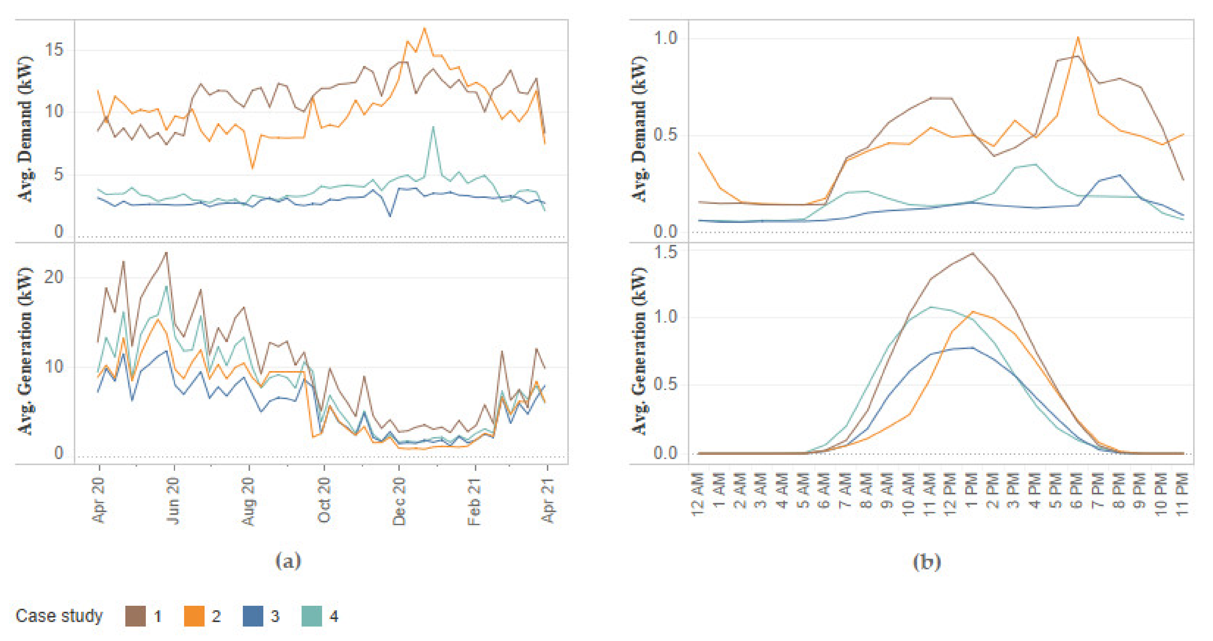
2.1.1. Case Studies

The analysis presented in this paper is based on a year-long monitoring study that involved four dwellings in or near Cardiff, South Wales, UK (SW). All dwellings were two storeys, either semi-detached or terraced buildings, and possessed an on-grid PV system of between 2 kWp and 4 kWp. All of the systems had been installed between 5 and 10 years before the start of the data collection. All houses were in urban areas, owner-occupied, and presented Energy Performance Certificates (EPC) level C or D. Two of the dwellings were inhabited by three or more residents (case studies 1 and 2), and two were inhabited by single residents (case studies 3 and 4).

2.1.2. Data Collection

The open-energy monitors model Emon TX v2 and current clamp sensors were used to record (1) imports from the grid, I, in kW; (2) exports to the grid, E, in kW; (3) PV generation G, in kW; and (4) total electricity demand, D, in kW. The data were collected using two sensors per dwelling, following the hardware setup suggested by the manufacturer [55], which was used to calculate the set of electricity balance variables using standard calculations methods found in the literature [25,31,56,57]. Figure 1 presents a diagram of the electricity flows considered for the analysis, and Figure 2 presents a conceptual graph of the different balance scenarios derived from the dwellings’ electricity balance.

2.1.3. Sampling and Analysis Intervals

Data were obtained using 10 s sampling intervals. More than 12 million data points were collected across the four houses, which were subsequently aggregated into 5 min intervals for postprocessing if required, and into 30 min intervals for the carbon emissions analysis. Figure 3 presents the daily and annual electricity demand and generation profiles of the dwellings.

2.1.4. Data Verification and Preparation

Whenever the data collection was interrupted, the whole day was discarded. This operation resulted in 89 discarded days out of a total of 1460 days of monitoring. Discarded dates were repopulated with the month’s average half-hourly values for that dwelling to prevent voids in the dataset. In one case, more than three consecutive weeks were missing in one dwelling, in which case the data were completed using the seasonal half-hourly averages.

Monthly readings from the utility meters were taken during the monitoring period to track possible mismatches, and minor corrections were applied where necessary. Monthly average differences between the monitored data and the utility meters data after the corrections were of 1.85% (+/−1.16%) for the generation and 0.18% (+/−2.72) for the import from the grid. Checks could not be performed for generation in one dwelling, since it did not possess a generation meter. The internal consistency of the data was checked using the energy balance assumptions that total generation plus total imports equal total exports plus total consumption, while at the same time, total self-consumption should equal generation minus exports and total consumption minus imports. No errors greater than 0.3% were found.

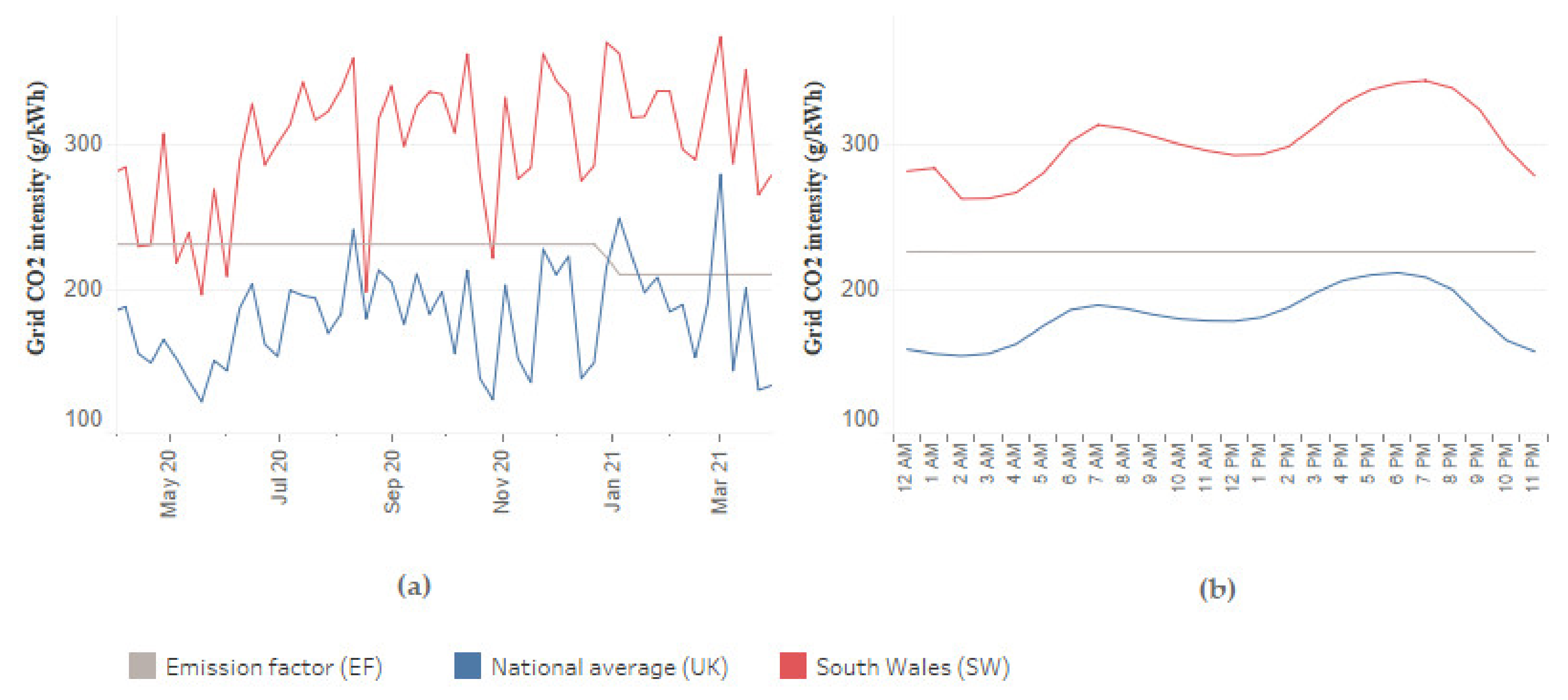
2.2. Secondary Data: Grid Carbon Intensity Data

Three different sources for the grid’s carbon intensity C (i) were considered: UK average national time-varying data, SW regional time-varying data [52,53], and DEFRA’s official emission factor (EF) [54]. Time-varying data were obtained from the national grid’s carbon intensity Application Programming Interface (API) on a 30 min resolution. Electricity EFs were taken as constants for each calendar year. Variations of the intensity values of each source of data are plotted in Figure 4.

The grid’s carbon intensity API service uses CO₂ g/kWh as its only metric and does not consider more comprehensive units such as CO₂ eq [52,53]. For this reason, all calculations in this study were performed using kg of CO₂ as the target unit. DEFRA’s EF of 231.04 g/kWh for 2020 and 210.16 g/kWh for 2021 [54] were considered as constants for the calculations.

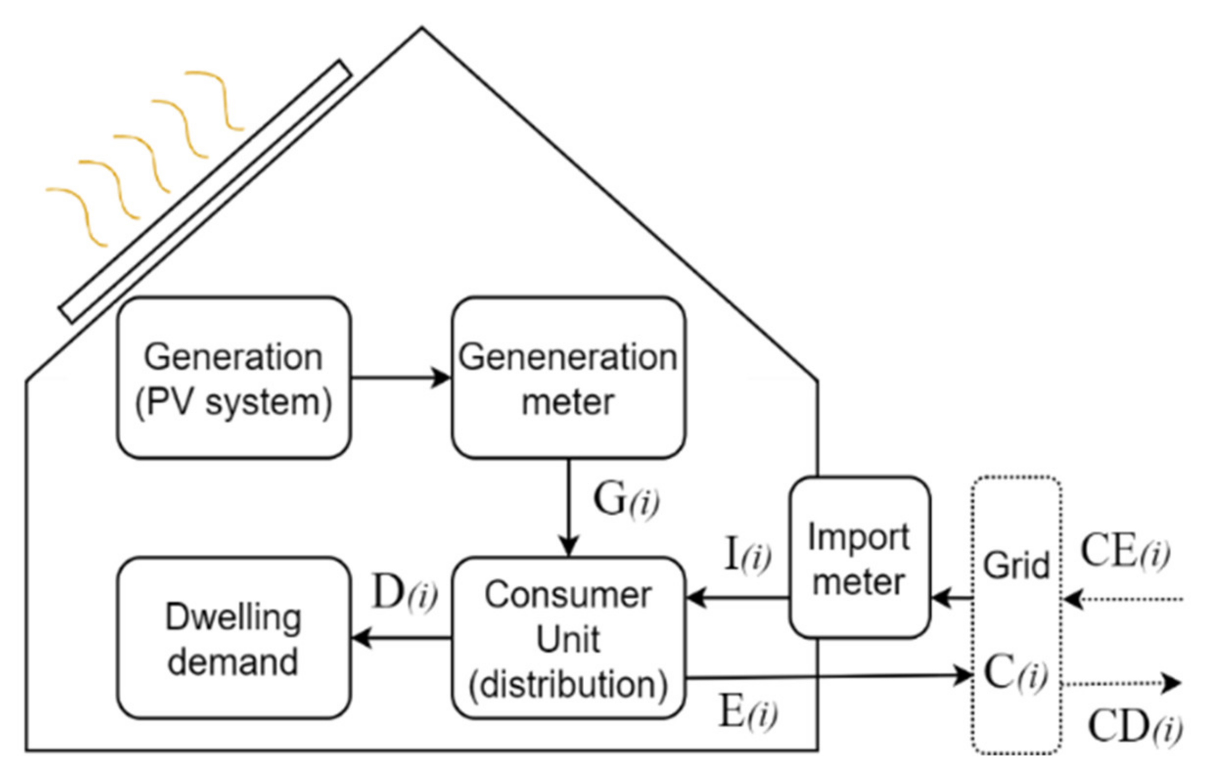
2.3. Carbon Emissions Variables

A dynamic approach was taken for the calculations, on which emissions were obtained considering the dwellings’ grid interaction situation (import/export) and multiplying it by the grid intensity levels at each time interval (i). In this way, electricity carbon emissions metrics (1)–(4) were calculated following the energy balance formulas proposed by Salom et al. [31,32]. For aggregations, index i was replaced by the period T, as presented in (5). The considered carbon emissions variables are:

• Gross carbon emissions (emissions produced off-site due to on-site grid imports):

$$C{E}_{\left(i\right)}={\mathrm{I}}_{\left(i\right)}\times {\mathrm{C}}_{\left(i\right)}$$

(1)

2.

Displaced carbon emission (emissions avoided off-site due to injections to the grid):

$$C{D}_{\left(i\right)}={\mathrm{E}}_{\left(i\right)}\times {\mathrm{C}}_{\left(i\right)}$$

(2)

3.

Referential emissions (or “functional equivalent emissions”):

$$R{E}_{\left(i\right)}={\mathrm{D}}_{\left(i\right)}\times {\mathrm{C}}_{\left(i\right)}$$

(3)

4.

Net emissions (or “emissions balance”):

$$NetC{E}_{\left(i\right)}=C{E}_{\left(i\right)}-C{D}_{\left(i\right)}$$

(4)

Equation (5) shows the calculation used for aggregations. A period T was defined to represent the timespan of the aggregation: 30 min, 1 h, 1 day, 1 month, or 1 year. Then, considering that N = T/i, the aggregated value of an expression x, such as CE, at the dwelling over a period was calculated as:

$$x_T={\displaystyle \sum }_{n=i}^{i+N}{x}_{\left(i\right)}$$

(5)

The same aggregation method was applied to all of the carbon emissions variables introduced between Equations (1) and (4).

2.4. Load-Matching Indicators

Four load-matching indicators were calculated to analyse whether their variations were associated with the variations in final carbon emissions. Two were associated with self-consumption, and two with daytime consumption.

Self-consumption “SC” is the energy produced on-site that is directly demanded on-site [28,31,57]. To calculate this, a logic conditioner needs to be taken into account, depending on the balance situation of the dwelling energy system, which can be one of three different situations, as shown in Figure 2. Then, self-consumption (kWh) is calculated as:

$$\begin{gathered} {\mathrm{G}}_{\left(i\right)}=0 \to S{C}_{\left(i\right)}=null \\ {\mathrm{G}}_{\left(i\right)}>D_{\left(i\right)}\to S{C}_{\left(i\right)}={\mathrm{D}}_{\left(i\right)} \\ {\mathrm{G}}_{\left(i\right)}<{\mathrm{D}}_{\left(i\right)}\to S{C}_{\left(i\right)}={\mathrm{G}}_{\left(i\right)} \end{gathered}$$

(6)

Self-consumption is usually represented as a ratio, but as McKenna et al. [57] point out, the ratio needs to be calculated from the aggregated values of self-consumption “SC” and generation “G (i)” during the evaluation period T. Otherwise, if it is obtained as the average of ratios, significant errors might occur. Therefore, the self-consumption ratio “SCR” can be assessed as an instant measurement obtained with instant values at any given sampling interval i, or as a ratio over a longer period, ideally a year, to account for seasonal variations [57], as shown in (7). Then, self-consumption ratio “SCR”, during an evaluation period T, such as a day, a month, or the whole year is calculated as follows:

$$SC{R}_T=\frac{{{\displaystyle \sum }}_i^{i+N}S{C}_{\left(i\right)}\times 100}{{{\displaystyle \sum }}_i^{i+N}{\mathrm{G}}_{\left(i\right)}}$$

(7)

The second indicator is the daytime consumption. McKenna previously proposed this measure [29] as the ratio of the total daily consumption that occurs between 10 am and 4 pm. This is an approximate calculation of the part of a day’s energy consumption that happens between the daytime peaks of carbon emissions, considering the year average values (see Figure 3, right side). However, it is not an exact measure of consumption happening during daylight hours. McKenna’s research has shown that daytime consumption can work as a predictor for self-consumption levels [29].

Here, we proposed to calculate it as two different indicators: daytime consumption, as proposed by McKenna (8), and daylight-time consumption (9), which was considered as the part of the daily energy consumption that happened during daylight hours. Since daylight hours are variable across the year, they were identified as the hours during which the PV panels generation is above 0. Then, the daytime consumption ratio “DCR” is calculated as:

$$DC{R}_T=\frac{{{\displaystyle \sum }}_i^{i+N}{D}_{\left(a\right)}\times 100}{{{\displaystyle \sum }}_i^{i+N}{D}_{\left(i\right)}}$$

(8)

where the index (a) identifies all the intervals that occurred between peak hours, e.g., between 10 am and 4 pm, during an evaluation period (1 day, month, year). Additionally, the daylight time consumption ratio “LCR” is calculated as:

$$LC{R}_T=\frac{{{\displaystyle \sum }}_i^{i+N}{D}_{\left(di\right)}\times 100}{{{\displaystyle \sum }}_i^{i+N}{D}_{\left(i\right)}}$$

(9)

where the index (di) identifies all the intervals that occurred while G > 0. Similarly, as with self-consumption, ratios were calculated in relation to the demand over the evaluated period.

2.5. Software

The integrations of the datasets, aggregations, and carbon calculations were performed using Tableau Prep 2021 and Tableau Desktop 2021. Tableau is a data management and visualisation software specialised for the analysis of multidimensional datasets. Graphs and final data tabulations were performed either in Microsoft Excel or Tableau Desktop.

3. Results

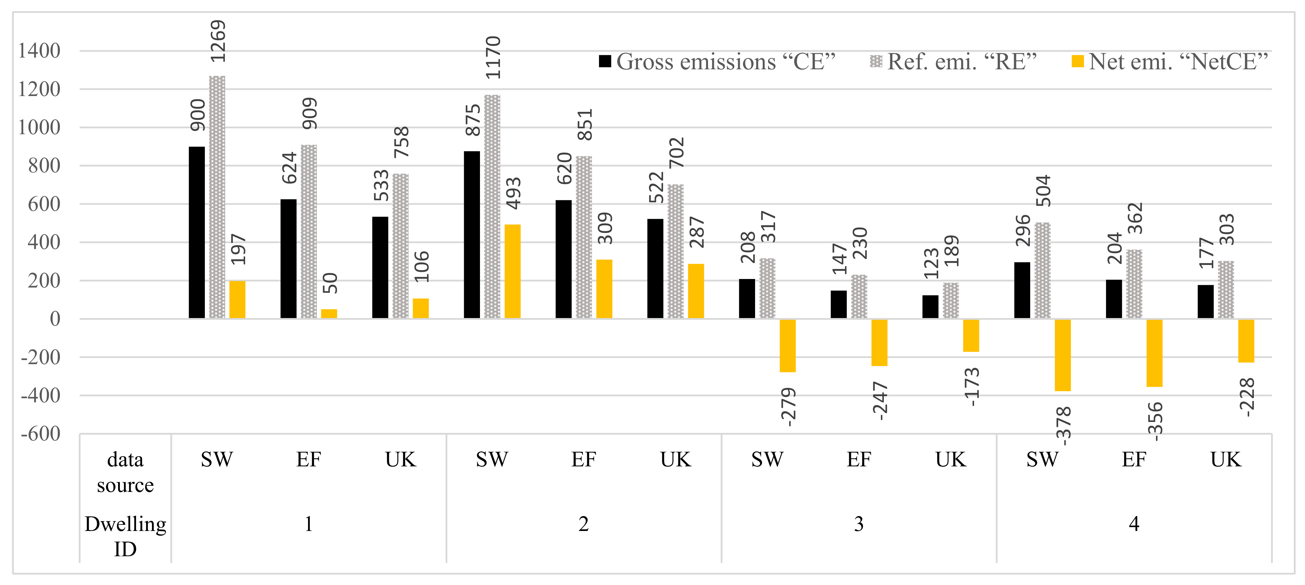
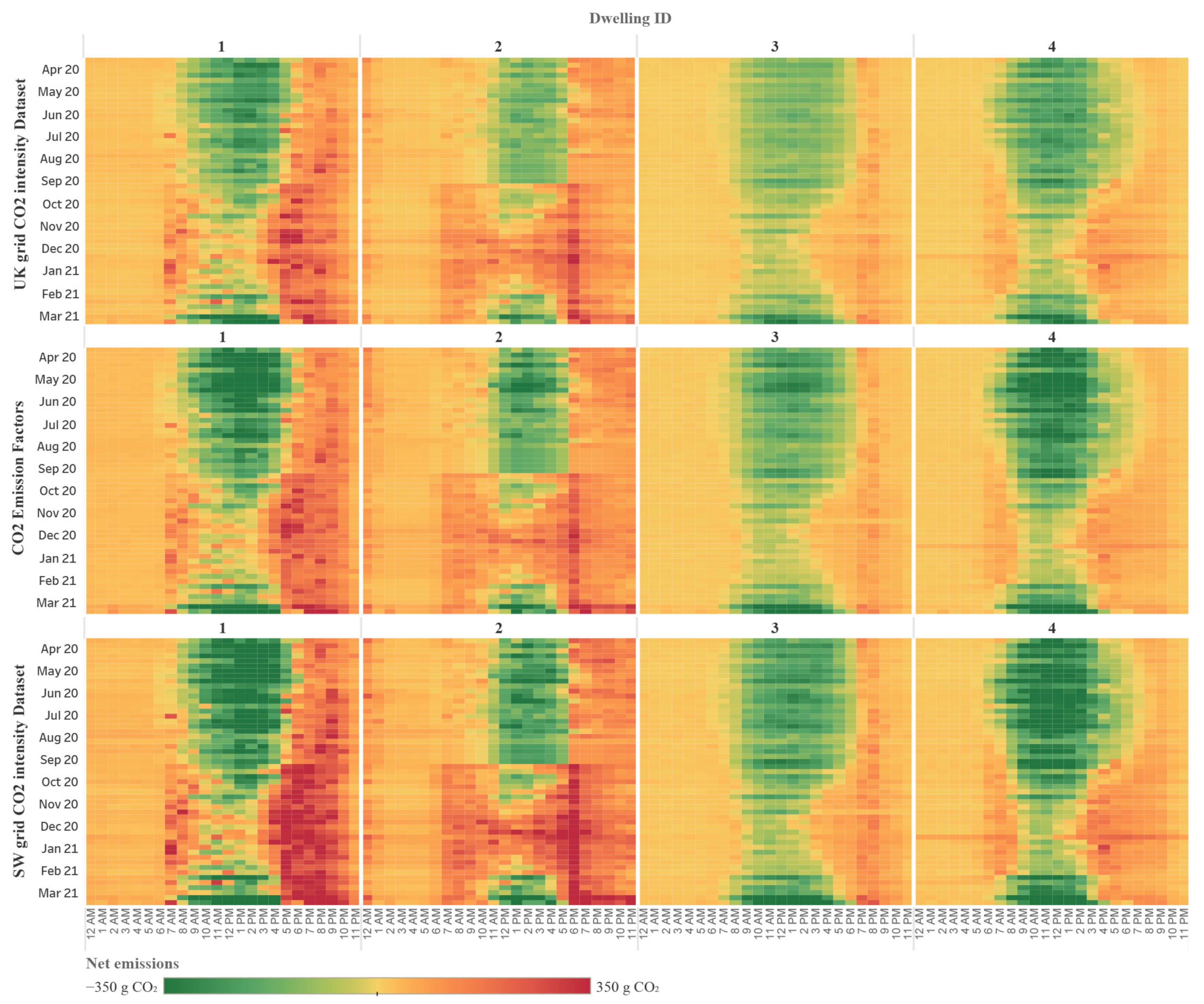
3.1. Reference, Gross and Net Carbon Emissions

Year total results are presented in Figure 5. The columns in black represent each dwelling’s yearly total gross emissions “CE”, in kg, calculated using each of the three data sources for grid emissions intensity. The columns in yellow represent the results of net emissions “NetCE”, in kg over the same year-long period. Finally, referential emissions “RE”, in kg are also provided, which are the emissions that each dwelling would have produced without the PV panels.

3.2. Differences in Carbon Emissions Totals across Data Sources

Table 4. Year total emissions displacements and gross and net emissions in kg.

Dwelling ID	CO2 Data Source	Emissions, Year Totals
		Displaced Emissions “CD” (kg/y)	Difference to EF (%)	Gross Emissions “CE” (kg/y)	Difference to EF (%)	Net Emissions “NetCE” (kg/y)	Difference to EF (%)
1	SW	702.4	22.3	899.6	44.1	197.2	294.0
	EF	574.3	0.0	624.4	0.0	50.0	0.0
	UK	427.5	−25.6	533.2	−14.6	105.7	111.2
2	SW	382.2	22.8	875.2	41.1	492.9	59.5
	EF	311.2	0.0	620.3	0.0	309.1	0.0
	UK	234.3	−24.7	521.7	−15.9	287.4	−7.0
3	SW	487.3	23.6	208.2	41.4	−279.1	13.0
	EF	394.1	0.0	147.2	0.0	−246.9	0.0
	UK	295.6	−25.0	123.0	−16.4	−172.6	−30.1
4	SW	673.6	20.4	295.9	45.1	−377.7	6.2
	EF	559.6	0.0	203.9	0.0	−355.7	0.0
	UK	404.8	−27.7	176.7	−13.4	−228.1	−35.9

shows the values obtained using each dataset for each dwelling. Percentual differences of each result if compared with the result obtained using the constant EF are provided.

Regarding gross emissions “CE”, the SW dataset produced the highest results across the four dwellings. The opposite happened with the UK dataset, which produced the lowest values across all dwellings. Variation across datasets was almost proportional regarding the gross emissions, with SW achieving between 41.1% and 45.1% more than EF in all cases, and the UK dataset achieving between −13.4% and −16.4%, respectively.

A similar trend was found in the net emissions “NetCE” calculations. Again, SW produced the higher results in all cases, while the lower results were produced by the UK dataset in three out of four dwellings. However, no consistency was found in the magnitude of the variations from EF in the “NetCE” calculation. The exception is case 1, where EF produced the lower results, and the variation rose to as high as 294% between the calculations performed with the SW and the EF datasets.

3.3. Differences in Comparative CO₂ Emissions Savings across Data Sources

Comparative CO₂ emissions savings were understood as the difference between the actual situation and the baseline situation. This can be observed in Figure 5, where the calculated emissions are plotted along with the baseline referential emissions “RE” value. RE corresponds to the emissions that the dwelling would have obtained if it did not have the PV system, i.e., the sum of emissions calculated using the total consumption at each given interval. Thus, comparative gross saved emissions (or reduced emissions) are defined here as the difference between the grey and the black columns of Figure 5 (the emissions which were avoided on-site due to the on-site direct consumption of PV generated electricity), whereas comparative net saved emissions are defined as the span between the grey and the yellow columns of Figure 5 (comparative gross saved emissions plus the emissions which were avoided off-site due to the energy injected to the grid). One interesting aspect of this graph is that in cases 2, 3, and 4, the comparative net saved emissions increased significantly with the more carbon-intensive datasets (SW and EF), despite the higher gross emissions. Another aspect is that dwelling 1 obtained markedly lower net emissions than dwelling 2, despite overall similar gross and reference emissions in both cases. To the best of the understanding of the authors, this difference is due to the bigger PV system size of dwelling 1, which implied larger amounts of energy being exported, and thus CO₂ being displaced off-site during idle hours.

Table 5. Year total comparative emissions savings in kg.

Dwelling ID	CO2 Data Source	Comparative Gross CO2 Savings		Comparative Net CO2 Savings
		(kg/y)	(%)	(kg/y)	(%)
1	SW	369.4	29.1	1071.8	84.5
	EF	284.9	31.3	859.3	94.5
	UK	224.6	29.6	652.1	86.1
2	SW	294.7	25.2	677.0	57.9
	EF	230.3	27.1	541.5	63.7
	UK	180.3	25.7	414.5	59.1
3	SW	108.5	34.3	595.7	188.2
	EF	82.9	36.0	477.0	207.3
	UK	66.1	35.0	361.7	191.2
4	SW	207.6	41.2	881.2	175.0
	EF	157.9	43.6	717.5	198.3
	UK	125.9	41.6	530.7	175.4

Highest values for each case have been highlighted in bold.

introduces the obtained values for net and comparative gross saved emissions using each dataset. It is highlighted that in all cases, SW produced the higher values of comparative gross saved emissions, whereas EF produced the higher percentual values of comparative net saved emissions. In all cases, comparative net savings were more than twice comparative gross savings, with a maximum difference registered in dwelling 4 using the EF dataset, where comparative net savings achieved a value almost six times higher.

The variation of net emissions obtained by each of the dwellings is presented in a set of carpet plots in Figure 6. Each of these plots shows the totality of the year for each dwelling using each of the carbon intensity sources. The most significant differences between datasets occurred in dwellings 1 and 2. Despite the fact that this was not statistically verified, it is possible to infer that these differences might be associated with (a) higher rates of the households’ peak demand matching the peak intensity hours of the grid and (b) differences in the rate of energy exported to the grid due to the dwellings’ different system sizes.

A trend that can be qualitatively recognised in Figure 6 is that the emissions displacements and thus comparative emissions savings were generally lower in the UK dataset case if compared to both SW and EF, which can be noticed in the lighter shade of greens showed during midday hours in the UK dataset plots. This is possibly because the “valley” in the grid carbon intensity between 10 a.m. and 4 p.m. (see Figure 4, right) had a much lower energy intensity in the UK dataset. Therefore, renewable sources generated high proportions of the grid’s electricity at some points in the summer, consequently making grid intensity during the valley hours become even lower than the year average. As a result, the exported energy became less carbon-intensive precisely in the moments of higher generation, displacing less carbon emissions. This raises questions regarding whether carbon displacements might become negligible in the near future once grid intensity approaches net zero carbon standards in the summer months.

3.4. Load-Matching Indicators Results

The rationale behind exploring the possible implications of load-matching indicators is that, on the contrary to the grid carbon intensity, these are values that are affected by the occupants’ activities. Therefore, they are subject to change with the householders’ demand management and lifestyle choices.

Table 6. Load-matching parameters, yearly results.

ID	Self-Cons. Ratio “SCR” (%)	Daytime Cons. Ratio “DCR” (%)	Daylight-Time Cons. Ratio “LCR” (%)
1	33.1%	31.1%	53.8%
2	42.4%	32.4%	55.1%
3	17.5%	28.9%	46.8%
4	22.1%	34.3%	62.1%

shows the main results of the considered load-matching indicators for each participant dwelling.

The annual self-consumption ratio observed in dwellings 1 and 2 were reasonably close to the average range found by McKenna, Pless, and Darby [57] in a UK nationwide study (37.3% ± 1.5%.) Nevertheless, the same variable in dwellings 3 and 4 were significantly below the national average, probably due to the single-resident composition of these households. All of the DCR values were above the reference band identified by [57] (between 25 and 28% for non prosuming dwellings), which means that the participants concentrated their energy demand during the midday off-peak hours to a greater extent than the UK average. It cannot be substantiated here whether this is due to a higher engagement of householders in energy demand management practices, but it could be the case. This observation is in line with the finding of McKenna, Pless, and Darby [57] that a larger proportion of PV users in the UK fell into this category and the fact that having PV systems might be a factor for demanding a higher amount of their total electricity consumption during the midday, or daytime, hours. The analysis of daylight-time consumption (LCR) shows different figures but a similar rank order across dwellings, with the notable exception of dwelling 4.

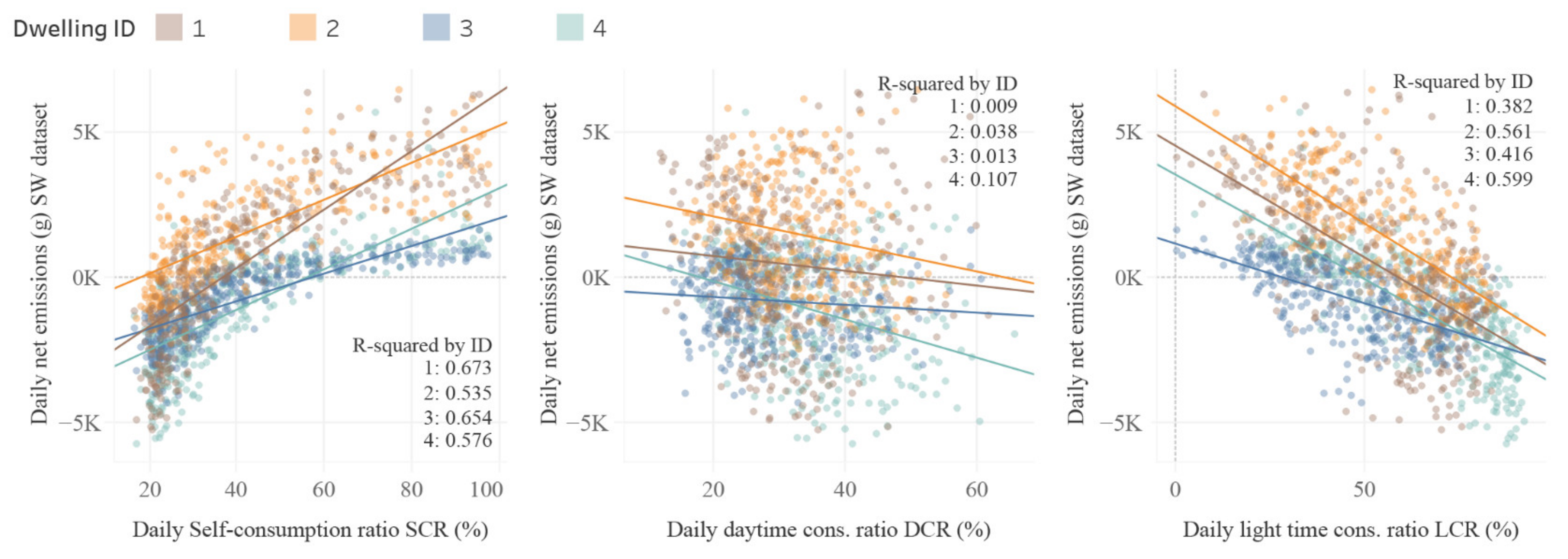
3.5. Association of Load-Matching and Emissions

Associations between the load-matching indicators (SCR, DCR, and LCR) and net emissions were studied using simple scatterplots and trend lines displayed in Figure 7. Grid intensity values from the SW dataset were used for the following calculation since, to the best understanding of the authors, this dataset should be considered the most accurate among the three consulted.

Daily net emissions were found to be related to the self-consumption ratio (SCR) but in a rather unexpected way. Since the SCR is a variable that has already been normalised by generation, a higher percentage of the SCR does not necessarily mean a higher figure of total self-consumed kWh. This implies that the days with higher self-consumption ratios are usually those with a lower level of generation, which is mostly self-consumed, so that the ratio is high, but the total self-consumed electricity in kWh is low. On the other hand, days with the highest generation achieve higher amounts of self-consumption in kWh but low levels of SCR. As a result, the relation found between SCR and daily net emissions was positive in all cases (Figure 7, left), which means that higher self-consumption was associated with days when the generation was not enough to cover the dwelling’s base demand.

The ratio of the total energy consumed between peaks, identified as the daytime consumption ratio (DCR), has been previously reported to be an important predictor for self-consumption in prosumer households [29,57]. Nevertheless, it was found that it had a low value as a predictor of final net emissions in the studied sample (Figure 7, centre). On the other hand, the daylight-time consumption ratio (LCR) was found to be inversely related to net emissions in a much more direct way than the daytime ratio (DCR) (Figure 7, right).

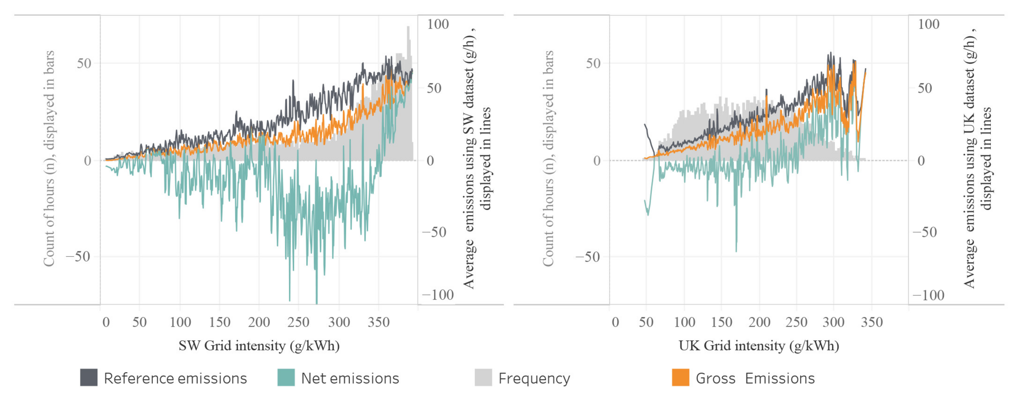
3.6. Association of Grid Intensity and Emissions

Finally, to better understand the relation between grid intensity and average emissions, the paper explored the average emissions (g/h) achieved across all dwellings for each level of grid intensity (g/kWh).

Results are plotted in Figure 8 considering the average results obtained when using each of the emission calculation methods: gross carbon emissions “CE”, reference emissions “RE”, and net emissions “NetCE”. In the graph, it is possible to observe that the average values of net emissions were highly volatile across most of the spectrum of grid intensity. Reference emissions and gross emissions averages became increasingly higher with higher intensities. Above 350 g/kWh in the SW case, or 250 g/kWh in the UK case, the trend also became apparent for net emissions.

This suggests that the grid’s carbon intensity values affect dwellings’ overall carbon emissions, despite the PV systems being in place, particularly when the grid intensity goes beyond a certain level (approx. 350 with SW and 250 with the UK data). This threshold, however, might be conditioned by the fact that the grid’s intensity goes up during peak demand times, mainly during the evening peak (4 to 9 PM, see Figure 4), while in the dwellings, the generation rate is usually low or null during these hours.

In both cases shown in Figure 8, SW and UK, the higher gross emissions (in orange) and net emissions (in turquoise) averages were concentrated in hours of higher intensity. However, net emissions reached considerably lower values when using the SW data. The study did not statistically test this, but to the best of the authors’ understanding, the differences are associated with the fact that most displacements were produced during midday hours, when the dwellings typically registered high generation and low consumption levels. This is exploratorily plotted in Figure 9.

Since the UK dataset displayed lower intensities than the SW dataset during midday periods, both displacements and peak emissions calculated using the UK dataset were always lower. This is translated in daily emission curves that directly resemble the famous California “duck curve” identified by the US’s National Renewable Energy Laboratory (ENRL) [58,59]. The duck curve highlights the rapid need for power in order to transit from a grid demand majorly covered by solar generation during midday hours towards a high demand peak intensity during early evenings. Whereas ENRL’s observation is made in relation to state-wide values, it is possible to observe here how the same issue affects prosumer buildings individually in their transition from a majorly self-consumer and net-exporter role during midday hours towards a majorly net-importer during the evenings. Whereas the duck curve’s multiple lines represent the variation in demand intensity throughout the years, in Figure 9, the lines represent differences in emissions produced by the different intensities of each of the sources of grid intensity values. From this observation, it becomes possible to suggest that if the grid carbon intensity becomes lower due to the higher penetration of solar generation in future years, operational net emissions of prosuming dwellings could tend to become higher due to an expectable reduction in the displaced emissions during midday hours.

4. Discussion

Four main aspects can be discussed from the results obtained by this study:

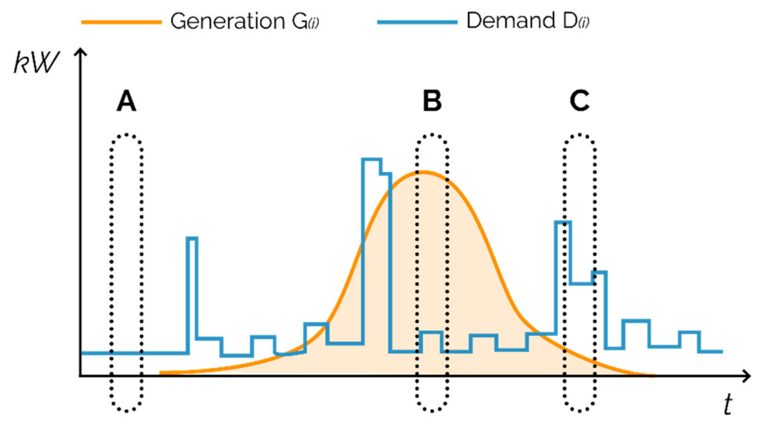
4.1. Relevance of the Hourly Variation of Intensity for the Final Emissions

The results showed that across the sample, the most significant part of the emissions came from demand occurring during high-grid-intensity hours, mainly during evening peaks (see Figure 9), and that to a greater extent, those evening emissions were compensated by the displacements produced by exports to the grid during midday idle periods (see Figure 6). As a result, net emissions show a value that is considerably lower than the actual gross emissions of the observed dwellings (see Table 4).

From this observation, it can be suggested that future grid scenarios with lower midday energy intensity, such as those aimed to be achieved by current decarbonisation policies and goals [5], may significantly affect the carbon emissions reduction potential of prosuming dwellings. This is particularly due to the possibility of net emissions becoming unbalanced if no demand management measures are implemented to match demand and generation times. In practical terms, if the average or sub-hourly emission factor (EF) reaches close-to-zero emissions levels during midday hours, the energy injected at that time will have minimum emissions displacement value. Despite being different in scope, similar observations regarding the impact of emission factors over emissions balance in future grids have already been suggested by Satola et al. [6], Parkin et al. [37], Noris et al. [60], and Schram et al. [38].

The implications of this observation might prove relevant not only for the management of carbon emissions in prosumer dwellings but also for the exploration of the impacts of electricity demand management for carbon emissions in the domestic sector as a whole, as suggested by Cozzi and Goodson [18], given that every dwelling is subject to the same hourly variations of the grid’s intensity of carbon emissions. The results from this study suggest that demand management could have a great impact if appropriately performed, which would be trying to shift demand from peak carbon intensity hours, which is when most of the emissions were produced (see Figure 8). However, as Egert et al. [19] suggest, given the volatile dynamics of the grid intensity, organising demand at the household level might only be possible with accessible communication of the grid CO₂ intensity information to final users.

Further lines of enquiry in this regard could relate to the quantification of the potential operational carbon emissions reductions that could be achieved by the implementation of demand-side management measures using expected future EFs of the electricity grid, comparing prosumer and non-prosumer dwellings scenarios. Similarly, comparing the potential emissions reductions to the embodied carbon emissions of on-site PV systems under future grid scenarios is another relevant research question.

4.2. Source of the Grid CO₂ Intensity Data Affects the Operational Emissions Values

The comparison between total net emissions values obtained using the different sources of grid intensity also showed that the use of the EF always produced higher percentual comparative savings (see Table 5). Differences of up to 290% in the resulting net emissions figures were found when the results obtained using the time-varying data were compared to the same calculations made using the EF (see Table 4, Case 1). On the other hand, the South Wales (SW) data always produced higher gross and net emissions totals. This leads us to consider two aspects.

Firstly, the outcome exemplifies the high variability of values that can be obtained depending on the EF data sources (mainly if time-varying vs. yearly EFs are considered) and calculation methodologies (gross emissions vs. net emissions). These results provide an empirical observation to support Satola et al. [6], Fawcett and Topouzi [35], and Lützkendorf and Frischknecht [33], who call for the necessity of standardising calculation and reporting methods. The results suggest that the standardisation could be extended to account for the type of data being used for the calculations.

Secondly, the fact that the geographical specificity of the data source produced differences in the emissions values of each dwelling raises some concerns, particularly since current operational emissions evaluation standards such as the widely used GHG protocol [40] call for the use of the most locally available data (i.e., the SW grid intensity data in this study). It has been observed that such an approach can create asymmetries for places where non-renewable high-power plants are located, such as South Wales, that still have plenty of gas-powered stations. Therefore, it was observed here that the final outcome of a building’s operational emission from electricity could depend more on its location than on its green credentials (efficiency rating, SAP, etc.) or the demand management practices of its users. This observation regarding the high relevance of location for final emissions aligns to those reached by the studies of Parkin et al. [6] and Schram et al. [38].

It is argued here that this situation is problematic since exactly the same buildings with exactly the same energy efficiency, generation, and use profiles would obtain different results simply because of the regional electric infrastructure, which creates an unjust situation. If such an approach to calculation became mandatory for building’s performance assessments, it would be “easier” to demonstrate low gross operational emissions in some places. This might not be too relevant under the current scenario, but if a higher portion of power demand becomes electrified (i.e., the wider deployment of EV and heat pumps), it could create significant differences in the yearly operational emissions only because of location. If such an approach were to be used for access to grants, certifications, or the definition of market desirability for buildings, the problem would become even more significant.

Further enquiry could focus on the analysis of the differences that would be obtained by using the different regional data sources provided by the UK’s National Grid to a single reference prosumer dwelling, to identify the geographical asymmetries and the linkages of this problem with the energy justice framework.

4.3. Relation between Operational CO₂ Emissions and Load-Matching Indicators Needs Further Investigation

The study explored the association between load-matching indicators and net emissions. An overall positive association of net emissions with self-consumption and a negative association with the daylight-time consumption ratio were found (see Figure 7, left and right). Nevertheless, none of them demonstrated a strong relationship. No clear relation was found between net emissions and daytime consumption ratio (see Figure 7, centre).

Further explorations and regression analysis based on larger datasets could help to clarify these trends. More detailed consideration might lead to identifying other factors or a combination of variables that could prove relevant as predictors of the final calculated emissions levels.

4.4. Metrics and Communication

This study also highlights the relevance of the reporting of emissions totals in association with other indicators, such as the use of both gross and net emissions, to provide a better representation of the dwellings’ CO₂ emissions intensity. It was observed that gross and net emissions could differ widely (see Table 4). Therefore, aligning to Bordass [34], who calls to move beyond single metrics assessments, it is proposed that both indicators are crucial to communicating buildings’ CO₂ emissions performance appropriately. By providing the gross emissions value, it is possible to understand the overall intensity of the operation and to what extent the electricity exports compensate that intensity. This is an intensity that becomes otherwise hidden if only net emissions are reported (see Appendix A).

Comparative saved emissions (on-site avoided emissions due to the direct demand of on-site generated electricity) were calculated using both gross and net emissions. Comparative net savings reached values twice or more times larger than comparative gross savings (see Table 5). These results allow us to argue that comparative gross and net savings approaches, even if declared as additional information, can be misleading and should be avoided.

Further work in this regard could explore the best ways to communicate and eventually reach combined gross and net operational emissions indexes for its use in scalable standards. The possibility of using dynamic methods such as the one presented in this paper to verify operational emissions obtained through ex-ante LCAs, also opens a relevant line of enquiry.

4.5. Limitations

A number of limitations need to be mentioned. Firstly, the fact that conclusions are drawn based on a sample of only four dwellings and that it only involved owner-occupied households needs to be taken into account. Secondly, the data collection period coincided with the first year of COVID-19 pandemic-related lockdowns, which might have affected the overall energy consumption routines of the studied households. Thirdly, the study only looked at the operational emissions during a year period and did not put these in relation to embodied emissions of the PV systems installation, nor in relation to the emissions of the complete operational stage of the systems. Similarly, other sources of CO₂ emissions produced during the period, such as gas consumption, are not accounted for. Fourth and lastly, the study used grid average emissions instead of marginal emissions to quantify the displacements and comparative savings due to limitations of the available data flows. The same calculations performed using marginal emission factors would arguably produce considerably higher total emissions and comparative savings results.

5. Conclusions

Operational CO₂ emissions from electricity balances in PV prosumer dwellings were calculated using empirical monitoring data and the electricity grid’s time-varying average CO₂ intensity values. Two time-varying sources of the grid’s CO₂ intensity were compared to the results obtained using the official yearly national average EF, all of which were valid for the location and timeframe analysed. Vast differences in the obtained operational CO₂ emissions values were found as a result of the used intensity data. Four different approaches to the calculation of emissions were adopted: gross emissions, net emissions, comparative emissions savings and comparative net emissions savings. In this regard, the results allow to question the usefulness of comparative savings and net saving approaches and highlight the relevance of considering the gross emissions for accurate communication of the building emission intensity. Three main recommendations arise from this study.

Firstly, given the variability of results obtained from the use of static and time-varying CO₂ intensity data sources, it is suggested that the use of time-varying data should be promoted to improve the precision of operational emissions accountancy, particularly in in-use verifications of buildings performance. However, the outcomes of this study also showed that the geographical boundaries of the intensity data can have a high impact on the results. It is suggested that the use of national time-varying averages should be preferred instead of regional ones, particularly in the definition of assessment frameworks and regulations, to avoid the generation of unjust situations concerning inequalities in the access to energy as a result of geographical conditions.

Secondly, the results highlight the relevance of promoting demand management policies and performance metrics that target reductions in buildings’ effective operational CO₂ emissions, instead of exclusively focusing on energy consumption and export balances. As it has been observed, net balances or reductions in energy consumption might not necessarily reflect the levels of reduction in gross CO₂ emissions when hourly fluctuations in the grid intensity are considered. However, it is acknowledged that such an approach would be conditioned to the rollout of smart meters or other on-site logging devices in participating buildings and the implementation of country-wide official information systems (user-accessible time-varying grid intensity data).

Finally, due to the evidenced high variation in results produced by the grid intensity data source, incorporating this criterion into standardisation efforts such as the “framework of different options for an energy or emissions balance” [6] is recommended. It is proposed that descriptors of the data source should consider at least the emission intensity data type (marginal or average), approach (location-based or market-based), the period covered by the factor (yearly ‘static’ factor, monthly, daily, hourly, etc.), and its geographical boundary (local, regional, or national).

References

1. UNEP-UN Environment Programme. United Nations Environmental Programme 2021 Global Status Report for Buildings and Construction: Towards a Zero-Emission, Efficient and Resilient Buildings and Construction Sector; UNEP: Nairobi, Kenya, 2021. [Google Scholar]
2. Bojek, P. Heymi Bahar Solar PV—Analysis. Available online: https://www.iea.org/reports/solar-pv (accessed on 29 January 2022).
3. IRENA—International Renewable Energy Agency. IRENA Renewable Power Generation Costs 2020; IRENA—International Renewable Energy Agency: Abu Dhabi, United Arab Emirates, 2020; p. 180. [Google Scholar]
4. Strielkowski, W.; Streimikiene, D.; Bilan, Y. Network charging and residential tariffs: A case of household photovoltaics in the United Kingdom. Renew. Sustain. Energy Rev. 2017, 77, 461–473. [Google Scholar] [CrossRef]
5. HM Government. Department for Business Energy & Industrial Strategy Net Zero Strategy: Build Back Greener; HM Government: London, UK, 2021; ISBN 978-1-5286-2938-6.
6. Satola, D.; Balouktsi, M.; Lützkendorf, T.; Wiberg, A.H.; Gustavsen, A. How to define (net) zero greenhouse gas emissions buildings: The results of an international survey as part of IEA EBC annex 72. Build. Environ. 2021, 192, 107619. [Google Scholar] [CrossRef]
7. Parag, Y.; Sovacool, B.K. Electricity market design for the prosumer era. Nat. Energy 2016, 1, 16032. [Google Scholar] [CrossRef]
8. Lowe, R.; Oreszczyn, T. Regulatory standards and barriers to improved performance for housing. Energy Policy 2008, 36, 4475–4481. [Google Scholar] [CrossRef]
9. DECC—Department of Energy & Climate Change. Feed-in Tariffs Scheme—Government Response to Consultation on Comprehensive Review Phase 2A: Solar PV Cost Control 2012; Department of Energy & Climate Change: London, UK, 2012.
10. Martin, N.; Rice, J. Solar Feed-In Tariffs: Examining fair and reasonable retail rates using cost avoidance estimates. Energy Policy 2018, 112, 19–28. [Google Scholar] [CrossRef]
11. Khodabakhsh, A.; Horn, J.; Nikolova, E.; Pountourakis, E. Prosumer Pricing, Incentives and Fairness. In Proceedings of the Tenth ACM International Conference on Future Energy Systems, Association for Computing Machinery, New York, NY, USA, 15 June 2019; pp. 116–120. [Google Scholar]
12. Sovacool, B.K.; Lipson, M.M.; Chard, R. Temporality, vulnerability, and energy justice in household low carbon innovations. Energy Policy 2019, 128, 495–504. [Google Scholar] [CrossRef]
13. Deng, G.; Newton, P. Assessing the impact of solar PV on domestic electricity consumption: Exploring the prospect of rebound effects. Energy Policy 2017, 110, 313–324. [Google Scholar] [CrossRef]
14. Tanaka, K.; Wilson, C.; Managi, S. Impact of feed-in tariffs on electricity consumption. Environ. Econ. Policy Stud. 2022, 24, 49–72. [Google Scholar] [CrossRef]
15. Kim, J.D.; Trevena, W. Measuring the rebound effect: A case study of residential photovoltaic systems in San Diego. Util. Policy 2021, 69, 101163. [Google Scholar] [CrossRef]
16. Galvin, R. I’ll follow the sun: Geo-sociotechnical constraints on prosumer households in Germany. Energy Res. Soc. Sci. 2020, 65, 101455. [Google Scholar] [CrossRef]
17. Galvin, R. Identifying possible drivers of rebound effects and reverse rebounds among households with rooftop photovoltaics. Renew. Energy Focus 2021, 38, 71–83. [Google Scholar] [CrossRef]
18. Cozzi, L.; Goodson, T. Empowering Electricity Consumers to Lower Their Carbon Footprint. Available online: https://www.iea.org/commentaries/empowering-electricity-consumers-to-lower-their-carbon-footprint (accessed on 8 June 2021).
19. Egert, R.; Daubert, J.; Marsh, S.; Mühlhäuser, M. Exploring energy grid resilience: The impact of data, prosumer awareness, and action. Patterns 2021, 2, 100258. [Google Scholar] [CrossRef] [PubMed]
20. Hansen, A.R.; Jacobsen, M.H.; Gram-Hanssen, K.; Friis, F. Three Forms of Energy Prosumer Engagement and Their Impact on Time-Shifting Electricity Consumption; ECEEE: Stockholm, Sweden, 2019. [Google Scholar]
21. Gram-Hanssen, K.; Hansen, A.R.; Mechlenborg, M. Danish PV Prosumers’ Time-Shifting of Energy-Consuming Everyday Practices. Sustainability 2020, 12, 4121. [Google Scholar] [CrossRef]
22. Kanakadhurga, D.; Prabaharan, N. Demand side management in microgrid: A critical review of key issues and recent trends. Renew. Sustain. Energy Rev. 2021, 156, 111915. [Google Scholar] [CrossRef]
23. OECD/IPEEC. Building Energy Efficiency Taskgroup Zero Energy Building Definitions and Policy Activity: An International Review; OECD/IPEEC: Paris, France, 2018. [Google Scholar]
24. Marszal, A.J.; Heiselberg, P.; Bourrelle, J.S.; Musall, E.; Voss, K.; Sartori, I.; Napolitano, A. Zero Energy Building—A review of definitions and calculation methodologies. Energy Build. 2011, 43, 971–979. [Google Scholar] [CrossRef]
25. Sartori, I.; Napolitano, A.; Voss, K. Net zero energy buildings: A consistent definition framework. Energy Build. 2012, 48, 220–232. [Google Scholar] [CrossRef] [Green Version]
26. Deng, S.; Wang, R.Z.; Dai, Y.J. How to evaluate performance of net zero energy building—A literature research. Energy 2014, 71, 1–16. [Google Scholar] [CrossRef]
27. Aelenei, L.; Aelenei, D.; Cubi, E.; Musall, E.; Jun Tae, K. Net Zero Energy Building Design Fundamentals. In Solution Sets for Net Zero Energy Buildings: Feedback from 30 Net ZEBs Worldwide; SHC—Solar Heating & Cooling Programme; Aelenei, D., Aelenei, L., Eds.; Ernst & Sohn: Berlin, Germany, 2017; pp. 7–37. ISBN 978-3-433-03072-1. [Google Scholar]
28. Luthander, R.; Widén, J.; Nilsson, D.; Palm, J. Photovoltaic self-consumption in buildings: A review. Appl. Energy 2015, 142, 80–94. [Google Scholar] [CrossRef] [Green Version]
29. McKenna, E.; Webborn, E.; Leicester, P.; Elam, S. Analysis of International Residential Solar PV Self-Consumption. In ECEEE 2019 Summer Study Proceedings; ECEEE: Stockholm, Sweden, 2019. [Google Scholar]
30. Gautier, A.; Hoet, B.; Jacqmin, J.; Van Driessche, S. Self-consumption choice of residential PV owners under net-metering. Energy Policy 2019, 128, 648–653. [Google Scholar] [CrossRef] [Green Version]
31. Salom, J.; Widén, J.; Candanedo, J.; Sartori, I.; Voss, K.; Marszal, A.J. Understanding Net Zero Energy Buildings: Evaluation Of Load Matching And Grid Interaction Indicators. In Proceedings of the Building Simulation 2011, Sydney, Australia, 14–16 November 2011. [Google Scholar]
32. Salom, J.; Widén, J.; Candanedo, J.; Lindberg, K.B. Analysis of grid interaction indicators in net zero-energy buildings with sub-hourly collected data. Adv. Build. Energy Res. 2015, 9, 89–106. [Google Scholar] [CrossRef]
33. Lützkendorf, T.; Frischknecht, R. (Net-) zero-emission buildings: A typology of terms and definitions. Build. Cities 2020, 1, 662–675. [Google Scholar] [CrossRef]
34. Bordass, B. Metrics for energy performance in operation: The fallacy of single indicators. Build. Cities 2020, 1, 260–276. [Google Scholar] [CrossRef]
35. Fawcett, T.; Topouzi, M. Residential retrofit in the climate emergency: The role of metrics. Build. Cities 2020, 1, 475–490. [Google Scholar] [CrossRef]
36. Connors, S.; Martin, K.; Adams, M.; Kern, E.; Asiamah-Adjei, B. Emissions Reductions from Solar Photovoltaic (PV) Systems; Laboratory for Energy and the Environment; Massachusetts Institute of Technology: Cambridge, MA, USA, 2004. [Google Scholar]
37. Parkin, A.; Herrera, M.; Coley, D.A. Net-zero buildings: When carbon and energy metrics diverge. Build. Cities 2020, 1, 86–99. [Google Scholar] [CrossRef]
38. Schram, W.; Louwen, A.; Lampropoulos, I.; Van Sark, W. Comparison of the Greenhouse Gas Emission Reduction Potential of Energy Communities. Energies 2019, 12, 4440. [Google Scholar] [CrossRef] [Green Version]
39. Asdrubali, F.; Baggio, P.; Prada, A.; Grazieschi, G.; Guattari, C. Dynamic life cycle assessment modelling of a NZEB building. Energy 2020, 191, 116489. [Google Scholar] [CrossRef]
40. World Resources Institute; Greenhouse Gas Protocol. Scope 2 Guidance. 2015. Available online: https://ghgprotocol.org/scope_2_guidance (accessed on 24 January 2022).
41. Almer, C.; Winkler, R. Analyzing the effectiveness of international environmental policies: The case of the Kyoto Protocol. J. Environ. Econ. Manag. 2017, 82, 125–151. [Google Scholar] [CrossRef] [Green Version]
42. RICS. RICS Whole Life Carbon Assessment for the Built Environment; RICS Professional Standards and Guidance; RICS: London, UK, 2017. [Google Scholar]
43. DEFRA. Guidance on How to Measure and Report Your Greenhouse Gas Emissions; DEFRA: London, UK, 2009; p. 75.
44. Government Property Agency. Net Zero and Sustainability Design Guide—Net Zero Annex. 2020. Available online: https://assets.publishing.service.gov.uk/government/uploads/system/uploads/attachment_data/file/925231/Net_Zero_and_Sustainability_Annex__August_2020_.pdf (accessed on 24 January 2022).
45. UKGBC. Renewable Energy Procurement & Carbon Offsetting Guidance for Net Zero Carbon Buildings; UKGBC: London, UK, 2021. [Google Scholar]
46. Bettle, R.; Pout, C.H.; Hitchin, E.R. Interactions between electricity-saving measures and carbon emissions from power generation in England and Wales. Energy Policy 2006, 34, 3434–3446. [Google Scholar] [CrossRef]
47. Corradi, O. ElectricityMap—Marginal Emissions: What They Are, and When to Use Them. Available online: https://electricitymap.org/blog/marginal-emissions-what-they-are-and-when-to-use-them/ (accessed on 29 January 2022).
48. Ascui, F.; Brander, M.; Cojoianu, T.; Li, Q. Moral Hazard and the Market-Based Method: Does Using Renewable Energy Attributes in Emissions Reporting Affect Corporate Emissions Performance? Social Science Research Network: Rochester, NY, USA, 2020. [Google Scholar]
49. Sotos, M.E. Scope 2: Changing the Way Companies Think About Electricity Emissions; World Resources Institute: Washington, DC, USA, 2015. [Google Scholar]
50. Department for Business, Energy & Industrial Strategy. Fuel Mix Disclosure Data Table. Available online: https://www.gov.uk/government/publications/fuel-mix-disclosure-data-table (accessed on 29 January 2022).
51. Qvist, F. ElectricityMap—How We Run the ElectricityMap Data Pipeline at Scale in the Cloud. Available online: https://electricitymap.org/blog/data-pipeline/ (accessed on 29 January 2022).
52. Alasdair, B.; Lyndon, R.; National Grid ESO UK. Environmental Defense Fund; University of Oxford; World Wildlife Fund Carbon Intensity. Available online: https://carbonintensity.org.uk/ (accessed on 6 November 2019).
53. Bruce, A.; Lyndon, R.; James, K.; Fraser, M.; Alex, R. Carbon Intensity Methodology: Regional Carbon Intensity; National Grid ESO: Warwick, UK, 2020. [Google Scholar]
54. DBEIS. DEFRA Government Conversion Factors for Company Reporting of Greenhouse Gas Emissions. Available online: https://www.gov.uk/government/collections/government-conversion-factors-for-company-reporting (accessed on 5 May 2021).
55. Hudson, G. Solar PV. Available online: http://guide.openenergymonitor.org/applications/solar-pv/ (accessed on 1 July 2021).
56. Salom, J.; Marszal, A.J.; Widén, J.; Candanedo, J.; Lindberg, K.B. Analysis of load match and grid interaction indicators in net zero energy buildings with simulated and monitored data. Appl. Energy 2014, 136, 119–131. [Google Scholar] [CrossRef]
57. McKenna, E.; Pless, J.; Darby, S.J. Solar photovoltaic self-consumption in the UK residential sector: New estimates from a smart grid demonstration project. Energy Policy 2018, 118, 482–491. [Google Scholar] [CrossRef]
58. NREL. Ten Years of Analysing the Duck Chart: How an NREL Discovery in 2008 Is Helping Enable More Solar on the Grid Today. Available online: https://www.nrel.gov/news/program/2018/10-years-duck-curve.html (accessed on 28 January 2022).
59. CAISO. Fast Facts: What the Duck Curve Tells Us about Managing a Green Grid; California ISO (California Independent System Operator): Folsom, CA, USA, 2016. [Google Scholar]
60. Noris, F.; Musall, E.; Salom, J.; Berggren, B.; Jensen, S.; Lindberg, K.; Sartori, I. Implications of weighting factors on technology preference in net zero energy buildings. Energy Build. 2014, 82, 250–262. [Google Scholar] [CrossRef]
Figure 1. Electricity balance monitoring framework for the studied dwellings, where G (i), I (i), E (i), and D (i) correspond to the logged parameters in kWh during sampling intervals i. Three sources for grid carbon intensity C (i) were used (UK, SW and EF), to obtain carbon emissions (CEs) (i) and carbon emissions displacements (CDs) (i).
Energies 15 02349 g001
Figure 2. Conceptual graph of the variation of demand D (i) and generation G (i) in a prosumer dwelling during a day. Three possible situations are recognised. (A) G = 0, all electricity comes from the grid; (B) G > D, demanded energy comes from the on-site system and excess are feed into the grid; (C) D > G, all site generation is consumed on-site plus a surplus from the grid.
Energies 15 02349 g002
Figure 3. Yearly variation of weekly average daily totals (a) and average daily variation of hourly totals (b) of total electricity demand “D” (kW) and generation “G” (kW) for the 4 case studies. Dwellings 1 and 2 correspond to multiple occupancy, whereas 3 and 4 correspond to single residents. The aggregation period T is daily at the left-side diagrams and hourly at the right-side diagrams.
Energies 15 02349 g003
Figure 4. Yearly variation of weekly average daily totals (a) and average daily variation of hourly totals (b) of the grid’s carbon emission intensity C (i) in g/kWh for the three consulted data sources.
Energies 15 02349 g004
Figure 5. Total calculated carbon emissions (kg) during the year period for the four dwellings (14), using the three available sources of the grid’s carbon intensity (SW: South Wales time-varying average, EF: emission factor, and UK: national time-varying average) and two calculation methods (gross emissions and net emissions). Referential emissions values are also provided, which are the emissions that each dwelling would have produced without the PV panels, obtained as presented in Equation (3).
Energies 15 02349 g005
Figure 6. Carpet plots of calculated net carbon emissions in each of the considered situations. In the distribution of plots rows are grid intensity data sources (UK, SW, and EF), and columns are case-study dwellings (14). In each plot, columns represent the progression of a day, hour-by-hour, while rows represent the progression of the year, week-by-week. Each cell represents the average net carbon emissions value for an hour of the day during each week of the year.
Energies 15 02349 g006
Figure 7. Associations between normalised daily load-matching parameters (x-axis) and net emissions (y-axis). Each point represents a day, and colours represent dwellings.
Energies 15 02349 g007
Figure 8. Average emissions across the 4 dwellings for each emission intensity value of the grid, calculated over hourly periods. Lines represent average of reference emissions (RE), net emissions (NetCE), and gross emissions (CE); bars present the frequency of occurrence of each grid intensity, counted in hours. (Left) represents the SW dataset; (right) represents the UK dataset.
Energies 15 02349 g008
Figure 9. Average daily variation of net emissions and export (kWh) per dwelling. It can be seen how emissions displacements (negative net emissions) become considerably higher during peak generation times. The higher overall grid intensity levels of the SW dataset mean that it achieves both higher minimum (midday) and maximum (evenings) levels.
Energies 15 02349 g009