Prediction Model for the Viscosity of Heavy Oil Diluted with Light Oil Using Machine Learning Techniques

Abstract

Due to the presence of asphaltene, the flow assurance of high viscosity crude oil becomes more challenging and costly to produce in wellbores and pipelines. One of the most effective ways to reduce viscosity is to blend heavy oil with light oil. However, the viscosity measurement of diluted heavy crude is either time-consuming or inaccurate. This work aims to develop a more accurate viscosity model of diluted heavy crude based on machine learning techniques. A multilayer neural network is used to predict the viscosity of heavy oil diluted with lighter oil. The input data used in the training include temperature, light oil viscosity, heavy oil viscosity, and dilution ratio. In this modeling process, 156 datasets were retrieved from the available iterature of various heavy-oil fields in China. Part of the data (80%) is used to train the developed models using Adam optimizer algorithms, while the other part of the data (20%) is used to predict the viscosity of heavy oil diluted with lighter. The performance and accuracy of the machine learning models were tested and compared with the existing viscosity models. It was found that the new model can predict the viscosity of diluted heavy oil with higher accuracy, and it performs better than other models. The absolute average relative error is 10.44%, the standard deviation of the relative error is 8.45%, and the coefficient of determination is R² = 0.95. The viscosity predicted by the neural network outperformed existing correlations by the statistical analysis used for the datasets available in the literature. Therefore, the method proposed in this paper can better estimate the viscosity of diluted heavy crude oil and has important promotion value.

1. Introduction

Heavy crude oils represent an important energy resource. The need for heavy oil processing has increased in recent years worldwide, backed by higher demands for petroleum products in the face of declining light crude oil resources. Moreover, commercial interest has been developed in heavy oil production systems with the advent of improved drainage areas by drilling multilateral and horizontal wells and highly deviated wells at shallow reservoirs [1].

Compared to light crude oils, the production and processing of heavy oils in the pipeline and wellbores are challenging due to their very high molecular weight components such as asphaltene, resins, and waxes. Moreover, the presence of heteroatoms and metals makes asphaltene the most polar polycyclic aromatic hydrocarbon, leading to its self-association with the formation of a viscoelastic network of nanoaggregates resulting in a high viscosity of heavy crude oils [2,3,4,5]. The viscosity of heavy crude oils is in the range of 100–10,000 cp at room temperature, while the extra-heavy crude oils have viscosities greater than 10,000 cp. Generally, crude oil with a viscosity of 400 cp is the classical maximum desired pipeline viscosity that can be transported through pipelines [6,7,8]. The most widely used method of reducing heavy crude oil viscosity in the pipeline is by blending heavy crude oils with a lighter oil due to the polarity of lighter oils [9,10,11,12]. It is known that reducing the dynamic viscosity of the oil reduces the internal friction resistance in the oil, which can increase the mobility of crude oils [13,14]. Therefore, the prediction of diluted viscosity is important for the pumping, production, and transportation of heavy crude oils.

Many studies have been conducted to predict the viscosity of diluted heavy crude oil. These studies can be classified into two main categories: lab-scale experiments and empirical correlations. Both of these are described and compared in the following.

The diluted viscosity of crude oils is usually measured in the laboratory. Yaghi and Al-Bemani (2002) [15] experimentally studied the effect of blending with light crude on viscosity at 30 and 50 °C. The light crude was added to the heavy crude and sheared at 6000 rpm for 3 min. The result showed that the heavy crudes diluted with light oil behaved as non-Newtonian (27% light oil) and Newtonian (30% light oil) fluid at 30 °C. The viscosity of the Newtonian dropped to approximately 1000 cp and did not meet the need for pipeline transportation, whereas, the heavy behaved as a Newtonian fluid at all the fractions at 50 °C. The viscosity could be reduced to 300 cp with the addition of 30% light oil. The effect of light oil concentration on viscosity behavior has been studied to lower the viscosity of the heavy crude oil by Hasan et al. (2010) using the RheoStress RS100. It was found that the heavy crude blended with a limited amount of lighter crude oil could efficiently lower the heavy crude oil viscosity. The viscosity of heavy crude dropped from 10,000 to 1200 cp with the presence of 10% light oil and from 10,000 to 350 cp with the presence of 20% light oil in the mixture [16]. Although the measured viscosity was more accurate than the calculated viscosity, the experimental viscosity measurement required a higher workload and was more expensive.

Therefore, some authors have researched viscosity calculation models that can predict the viscosity of diluted heavy crude oil, since this method can effectively lower the experimental workload and improve work efficiency. The first correlation for predicting the viscosity of a mixture of two fluids was proposed by Arrhenius [17] in 1887. Although it was suggested for a mixture of two pure liquids, it is worth evaluating its capabilities in predicting the viscosity of heavy crude oil with a high viscosity ratio system. Subsequently, an exponential equation was presented by Kendall and Monroe [18] based on measurements of molar fractions. The comparison results showed it had a good fit with experimental viscosities. However, these models were not accurate for diluted heavy crude [19].

Cragoe [20] introduced a universal equation for binary heavy oil–solvent mixtures, which was a function of the mass fraction and the viscosity of the component. Later, the development of more complex equations, such as the four-parameter model, was developed to predict the viscosities of petroleum fractions blends. There were three methods in Al-Besharah’s [21] work: ASTM D341 [22], the Refutas index method [23], and a four-parameter model based on the Ratcliff and Khan [24] equation were compared. The results showed that the four-parameter model had the lowest errors. In 2019, Mohammadi [25] developed a new empirical model for measuring the kinematic viscosity of blends. The parameters of this model were obtained based on a genetic algorithm using 850 data points. In his work, the viscosity of a crude oil blend depended on the mass or volume fraction and viscosity of each component of the blend. However, it ignored the effect of temperature on the viscosity of blends.

Recently, Jing et al. [26] investigated the viscosities of two heavy oils diluted with five light oils from the published literature. The experimental and calculated viscosity in terms of the Lederer model, the Arrhenius model, the double logarithmic model, and the Crageo model were compared. It showed that the Cragoe model had the lowest average relative error and the maximum relative error. In addition, Xing [27] evaluated eight kinds of mature oil mixing viscosity models using experimental viscosities. The eight mixing viscosity models consisted of the Cragoe model, double logarithmic model, Lederer model, the Arrhenius model, the Kendal-Monroe model, etc. However, the results calculated by these models showed that the errors were very large. Therefore, the Arrhenius modified model III was proposed and had the lowest average absolute error of 6.9%. From these studies, it is found that existing viscosity models are limited and may not be applicable to other oilfields. Therefore, using artificial neural networks (ANNs) to predict the viscosity of heavy crude oil blended with light oils is the focus of this research.

Many researchers have summarized that ANNs can be a useful tool to model different engineering systems under real-world conditions, such as in solar energy systems [28], solar distiller [29,30,31], and petroleum engineering [32,33,34]. Compared with traditional methods, there is no need for ANNs to provide a model function and understand the input/output relationships before forecasting. The learning capability of an ANN has the chance to discover more complex and subtle interactions between the data of input and output. In addition, ANNs also present the potential for high fault tolerance in the wide ranges of variables [35,36,37].

Thus, this paper aims to develop a robust model using ANNs to predict the viscosity of diluted heavy crude oil sufficiently. To do so, we collected a total number of 156 viscosity datasets from openly published literature. Moreover, the prediction viscosity was also compared with some empirical correlations available in the literature.

2. Data and Methods

2.1. Data Collection

To achieve the objective of this paper, 156 viscosity experimental datasets of diluted heavy crude were collected from several different oil fields in China. Each heavy crude oil was blended with the light oil in different dilution proportions. The mixture was homogenized using a stirrer for 1 h and heated to a specific temperature. Then, the respective mixtures were left for 2 days to reach equilibrium; then, the viscosity of these crude oils was measured using a model VT550 viscometer (Thermo Fischer, Shanghai, China). The related parameters include heavy crude viscosity, light crude viscosity, dilution rate, and temperature.

Table 1. Characteristics of parameters.

Title 1	Title 2	Minimum Value	Maximum Value
1	Heavy crude viscosity, cp	121	4020.6
2	Light crude viscosity, cp	2.9	35.7
3	Dilution rate	0.2	0.9
4	Temperature, °C	20	60
5	Diluted heavy viscosity, cp	9.3	882

summarizes the main information of the parameters used in this study.

2.2. Artificial Neural Network Theory

A neural network is a series of algorithms that endeavors to perform pattern recognition, predictive evaluation, and evaluation analysis in datasets through a process that mimics the way the human brain operates. It contains layers of interconnected nodes. Each node is known as the perceptron, and a perceptron will take several inputs and produce a single output. Each of those perceptrons makes a decision by weighing the results from the first layer of decision making. The perceptron of the next layer (second, third, etc.) can engage in more complex decision making in this way. By varying the values of weights and the thresholds between elements, we can perform a specific function and compare the output and the target, until the network output matches. The schematic of the network can be seen in Figure 1.

The steps of the training process for the single-layer neural network are as follows:

① The weighted sum of the input signals can be calculated as:

$$v={\displaystyle {\sum }_1^n{X}_i{W}_{ii}+b}$$

(1)

② The output value is calculated using the activation function:

$$y_i=f(v)=f({\displaystyle {\sum }_1^n{X}_i{W}_{ii}+b})$$

(2)

③ The error of the output is calculated as:

$$e_i=y_{tar}-y_i$$

(3)

④ The updated weight is calculated using the delta rule:

$$W_{ii}\leftarrow W_{ii}+\Delta W_{ii}=W_{ii}+\alpha e_i{x}_i$$

(4)

⑤ Perform Steps ①–④ for all training samples.

⑥ Repeat Steps ①–⑤ until the error meets the requirements and obtains the predicted value.

2.3. Artificial Neural Network Construction and Optimization

To improve the generalization ability of the model, viscosity datasets obtained from published literature were used. They were randomly divided into two parts of which 80% was used for network training and 20% for network prediction accuracy test.

Due to the different ranges of the heavy crude viscosity, light oil viscosity, and diluted viscosity obtained by the experimental method, the first thing to do was to normalize all the datasets and map all the data to the interval [–1, 1]. The dimensional differences and magnitude differences between indicators could be eliminated by using the normalization method, so that data information could be mined more accurately and satisfactorily. This work adopted the data normalization method provided by scikit-learn, and its normalization formula is [38]:

$$x_{norm}=\frac{x_i-x_{\min }}{x_{\max }-x_{\min }}.$$

(5)

The network in this work used a five-layer neural network structure, that is, three hidden layers, one input layer, and one output layer. It is known that the viscosity decreases sharply with increasing temperature. In addition, the heavy crude viscosity, light oil viscosity, and dilution rate also play an important role in the diluted viscosity. Therefore, four input parameters and an output parameter were designed in our ANN structure. The input parameters included heavy crude viscosity, light crude viscosity, dilution rate, and temperature, while the output parameter was the viscosity of heavy crude oil diluted with light oil, thereby establishing a viscosity prediction model.

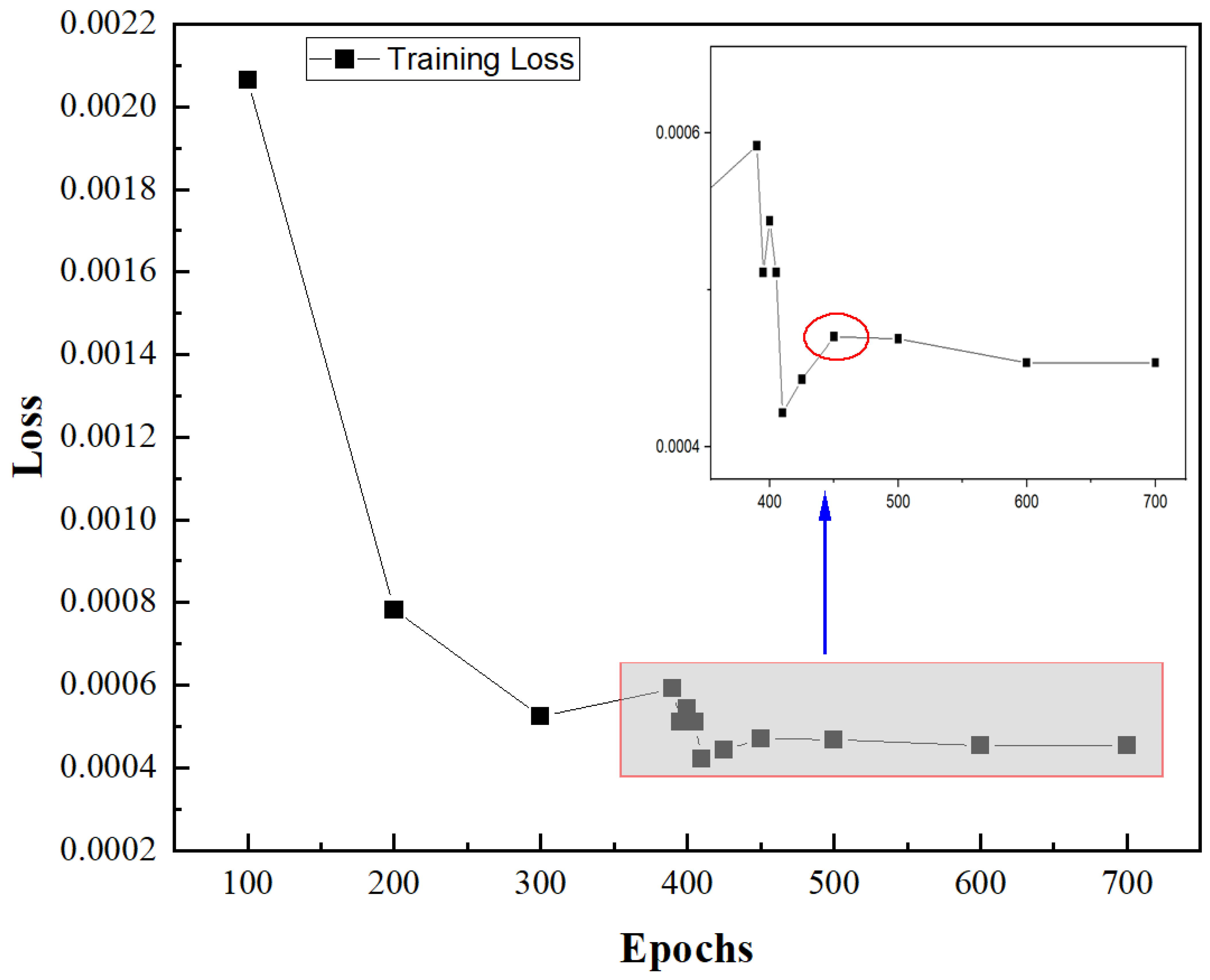
2.3.1. Neural Network Training Times

In this paper, the training times for the ANN were set from 100 to 700. The network corresponding to different training times is shown in Figure 2. According to the loss result, the loss decreased with time. When the training times reached 450, the loss was maintained at around 4.7 × 10⁻⁴, and the subsequent training basically stabilized. Therefore, the number of training times was set to 450.

2.3.2. Optimization Model

The error backpropagation was selected as a learning technique in this paper, since it can efficiently calculate gradient vector, computationally speaking. In addition, the adaptive moment estimation (Adam), stochastic gradient descent (SGD), and adaptive gradient algorithm (Adagrad) were used to calculate the loss in the training process. The results of the three optimizer algorithms are shown in Figure 3. It can be seen from the figure that with the change in time, the loss value of the Adam became the smallest, and the curve basically stabilized. Therefore, this paper chose the Adam optimizer algorithm to predict the viscosity of heavy oil diluted with light oils.

2.3.3. Execution Procedure

The execution procedures of the proposed ANN model are presented in Figure 4. The dataset was preprocessed and separated into a training and test set. The number of neurons in each layer and MinRMSE were initialized. Then, the ANN model was trained using the training set, and the RMSE was also calculated. The number of neurons of each layer was updated to minimize the RMSE. In addition, this paper assumed a maximum of 50 neurons per layer. Three sets of inner loops were used to screen out the optimal model with the MinRMSE. Once the best model was obtained, we tested the ANNs with the best model. Finally, the optimized ANNs were employed to predict the diluted viscosity of heavy oils.

The above analysis results show that the optimal number of neurons corresponding to the three hidden layers were 11, 11, and 11, respectively. In addition, the corresponding bias and weight are shown in

Table A1. The weight and bias results of the optimal model.

Layer	Weight	Bias
Input-Layer 1 (4 × 11)	[−0.26 −0.24 0.16 −0.2 −0.54 0.39 0.45 −0.15 0.09 −0.09 −0.32] [0.36 0.2 0.084 0.17 0.5 −0.73 0.15 −0.45 −0.43 0.14 −0.59] [0.45 −0.5 −0.13 −0.025 −0.26 −0.16 −0.51 −0.024 0.29 −0.39 0.15] [0.16 −0.38 0.4 −0.062 −0.24 −0.19 −0.35 −0.3 −0.41 0.4 −0.41]	[0.22 0.04 0.08 −0.01 0.14 0.26 −0.08 0.24 −0.17 0.08 0.17]T
Layer 1–2 (11 × 11)	[0.1 −0.045 −0.95 0.088 0.57 0.46 −0.12 −0.37 0.38 0.023 0.76] [0.003 −0.06 −0.059 0.29 0.29 0.32 0.46 0.31 −0.37 −0.12 −0.22] [0.81 0.29 −0.04 0.38 −0.61 −0.54 −0.095 0.32 −0.71 −0.77 0.23] [−0.18 −0.37 0.37 −0.15 0.43 0.35 0.097 0.21 0.041 −0.15 −0.57] [0.047 0.079 0.31 0.3 0.19 0.54 −0.038 −0.1 0.35 −0.39 −0.02] [0.26 −0.44 0.54 0.45 −0.11 0.29 0.17 −0.36 0.09 0.55 0.07] [0.28 0.4 −0.10 −0.13 −0.24 0.55 −0.15 −0.19 −0.21 0.37 −0.46] [0.06 −0.80 0.38 −0.06 0.27 0.15 0.28 −0.09 0.48 0.37 −0.53] [−0.25 0.28 −0.32 −0.29 −0.06 −0.39 −0.43 −0.25 −0.08 0.48 0.29] [0.21 0.32 −0.18 −0.26 −0.018 0.16 −0.25 −0.2 0.33 0.14 0.57] [−0.12 −0.49 −0.11 0.33 −0.05 −0.23 0.31 −0.14 −0.09 0.16 −0.46]	[−0.06 0.04 0.05 0.13 −0.02 0.17 0.15 −0.04 0.15 0.14 0.07]T
Layer 2–3 (11 × 11)	[−0.23 0.31 −0.41 0.16 −0.46 −0.24 −0.25 −0.41 0.14 0.65 −0.33] [−0.60 0.44 0.21 0.11 −0.42 0.21 −0.13 −0.38 −0.13 0.36 −0.38] [0.20 −0.32 0.26 0.51 0.41 0.50 0.42 −0.21 −0.18 −0.96 −0.01] [0.43 −0.49 −0.2 −0.38 −0.01 0.51 −0.31 0.13 −0.07 0.32 0.21] [0.49 0.22 0.36 −0.28 0.02 0.35 0.25 0.16 0.05 −1 0.21] [0.10 −0.48 −0.45 0.51 −0.12 0.5 −0.52 −0.23 −0.58 −0.27 0.17] [0.44 −0.12 0.07 −0.082 −0.5 0.33 −0.14 0.38 −0.10 −1 0.42] [0.17 0.42 −0.05 −0.46 −0.3 0.36 0.36 −0.10 0.12 −0.29 −0.2] [−0.45 0.25 0.05 0.46 −0.12 0.12 0.08 0.54 −0.13 −0.38 0.43] [0.09 0 −0.17 0.26 −0.22 0.04 0.03 −0.41 −0.41 −0.67 0.47] [0.19 −0.54 0.37 −0.43 −0.44 −0.58 −0.13 −0.2 0.16 0.75 0.15]	[−0.12 −0.05 −0.01 0.09 0 0.15 −0.03 0.16 −0.07 0.26 0.12]T
Layer 3-Output(11 × 1)	[0.73 0.14 −0.19 −0.08 −0.08 −0.41 0.28 −0.2 −0.46 0.83 −0.47]T	−0.07

, Appendix A.

Therefore, the optimal topology of this work is shown in Figure 5.

2.4. Statistical Error Analysis

To determine the ability and accuracy of the proposed viscosity model, cross plots and statistical methods, including the percentage average relative error (ARE%), the average absolute relative error (AARE), the mean absolute error (MAE), mean relative error (MRE), and the standard deviation (SD) were performed as shown in Equations (6)−(10), respectively. The arithmetic average of the absolute relative errors (AARE) is the difference in the magnitude between the measured and the predicted value of the model. A low value of AARE% means better results and is consistent with real values around the 45° line. The SD represents the deviation of the predicted values from the average result.

$$E_{ARi}=\frac{\left|{({\mu }_{Experimental})}_i-{({\mu }_{\mathrm{Pr}edicted})}_i\right|}{{({\mu }_{Experimental})}_i}\times 100$$

(6)

$$AARE=\overline{E_{ARi}}=\frac{{\displaystyle {\sum }_{i=1}^n{E}_{ARi}}}{n}$$

(7)

$$S{D}_{ARE}=\sqrt{\frac{{\displaystyle {\sum }_{i=1}^n{(E_{ARi}-\overline{E_{ARi}})}^2}}{n-1}}$$

(8)

$$MAE=\frac{1}{n}{\displaystyle \sum _{i=1}^n\left|{({\mu }_{Experimental})}_i-{({\mu }_{\mathrm{Pr}edicted})}_i\right|}$$

(9)

$$MRE=\frac{1}{n}{\displaystyle \sum _{i=1}^n\frac{\left|{({\mu }_{Experimental})}_i-{({\mu }_{\mathrm{Pr}edicted})}_i\right|}{{({\mu }_{Experimental})}_i}}$$

(10)

3. Results and Discussion

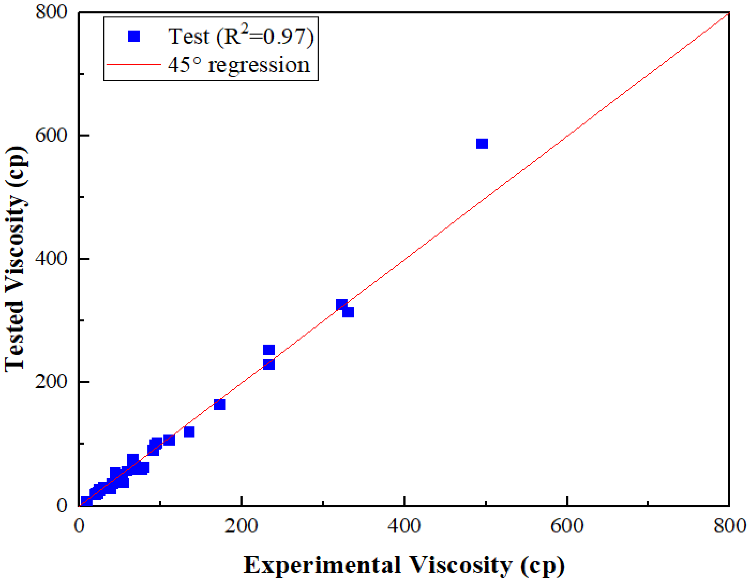
3.1. Prediction of Crude Oil Viscosity

Some of the viscosity correlations of heavy crude oil diluted with light oil were used in this paper. These correlations consisted of the Arrhenius’s correlation, double log correlation, Cragoe’s correlation, Kendal-Monroe’s correlation, and Xing’s correlation. The viscosity of diluted heavy crude oils can be calculated as follows:

Arrhenius (1887):

$$\begin{array}{l}\lg {\mu }_m=X_1\lg {\mu }_1+X_2\lg {\mu }_2\\ X_1+X_2=1\end{array}$$

(11)

Double log (1983):

$$\begin{array}{l}\lg \lg {\mu }_m=X_1\lg \lg {\mu }_1+X_2\lg \lg {\mu }_2\\ X_1+X_2=1\end{array}$$

(12)

Cragoe (1933):

$$\begin{array}{l}{\mu }_m=5\times {10}^{-4}\exp (1000\ln 20/L_m)\\ L_m=X_1{L}_1+X_2{L}_2\\ L_i=\frac{1000\ln 20}{\ln {\mu }_i-\ln (5\times {10}^{-4})}\end{array}$$

(13)

Kendal-Monroe (1917):

$${\mu }_m{}^{1/3}={\displaystyle \sum _{i=1}^n{x}_i}{\mu }_i{}^{1/3}$$

(14)

Xing (2021)

$$\begin{array}{l}{\mu }_m={(0.7-0.5X_1+0.01T)}^C\\ C={\displaystyle \sum _{i=1}^n{x}_i\lg }{\mu }_i\end{array}$$

(15)

3.2. Determination of the New Viscosity Model

To determine the accuracy of the ANN training values in predicting the viscosity of diluted heavy crude, the values of training and experimental are plotted in Figure 6. According to the trained value and statistical results, all the training viscosities were closer to the 45° line; in other words, they were close to the experimental viscosities. In addition, the viscosity values had a coefficient of determination R² of 0.99 between the training and experimental viscosity. Moreover, the result of the regression plot generated by this model showing the relationship between the tested and experimental viscosity values is shown in Figure 7. It can be seen that the tested viscosities were also closer to the 45° line, and the values had a coefficient of determination R² of 0.97. Therefore, it can be concluded that the model had a higher degree of fit and could predict the diluted viscosity satisfactorily.

Figure 8 shows the accuracy plot of the training and validation loss with relation to the number of epochs used for the development of the model.

3.3. Comparison of the ANN with Existing Empirical Correlations

This paper cited the experimental viscosity value of the heavy crudes mixed with light oils from the published literature. We compared the values of existing empirical correlations in Section 3.1, the proposed model in this work, and experimentally, in terms of their performance and accuracy with diluted heavy crude oils.

Figure 9 depicts a comparison between the calculated and experimental viscosities of different models. It can be seen that Kendal-Monroe’s and Arrhenius’s models significantly overestimated the viscosity of the diluted heavy crude, whereas Xing’s model predicted lower viscosities. It should be noted that Cragoe’s and double-log’s models had a better fit and a closer fitting slope, and the predicted viscosity data of the others were scattered. The reasons for the high prediction accuracy of the ANN model are as follows:

(1)

Compared with the Arrhenius, Double log, Cragoe, and Kendal-Monroe models, the new model considered the effect of temperature on viscosity, which increased the accuracy of the new model;

(2)

As for the Xing model, this model was developed on the basis of the Arrhenius model by introducing a correction coefficient. It can be seen from Figure 9 that the viscosity predicted by the Arrhenius model was larger than the measured viscosity, while the viscosity predicted by the new model was smaller than the experimental viscosity, which may be caused by an inappropriate correlation coefficient of the Xing model.

To determine the degree of prediction bias of the new method, the AARE and SD% of different models were also compared in Figure 10. It is clear from this that the proposed model provided the best prediction with the heavy crude oil diluted with light oils and performed very well against the other models. The newly developed model had the lowest AARE% of 10.45% and an SD% of 8.45%. The closer the errors are to 0, the more accurate the model. Considering that the datasets contained a wide range of viscosities, the model proposed in this paper had better prediction performance on the viscosity of heavy crude diluted with light oils.

4. Conclusions

In this paper, a novel method for predicting the viscosity of heavy crude oil diluted with lighter oils was proposed based on machine learning. The comparison between the prediction of the new correlations and the other empirical correlations available in the literature was carried out. Furthermore, the statistical error analysis was used to determine the accuracy of these correlations. The key findings of this novel viscosity model are summarized as follows:

(1)

From the analysis of the results, the new viscosity model had the lowest absolute average relative error values of 10.45%, standard deviation values of 8.45%, and coefficient of determination (R² = 0.95).

(2)

The new viscosity showed a good accuracy as well when compared to the conventional viscosity correlations in the published literature. In other words, the new viscosity model outperformed empirical correlations.

(3)

The presence of asphaltene in heavy crude oil is also an important parameter affecting the viscosity of the heavy crude oil, and it can be studied in future research.

References

1. Ramasamy, M. Processing of Heavy Crude Oils Challenges and Opportunities; IntechOpen: London, UK, 2019. [Google Scholar]
2. Taborda, E.A.; Alvarado, V.; Franco, C.A.; Cortes. Rheological demonstration of alteration in the heavy crude oil fluid structure upon addition of nanoparticles. Fuel 2017, 189, 322–333. [Google Scholar] [CrossRef]
3. Taborda, E.A.; Franco, C.A.; Ruiz, M.A.; Alvarado, V.; Cortes, F.B. Experimental and theoretical study of viscosity reduction in heavy crude oils by addition of nanoparticles. Energy Fuel 2017, 31, 1329–1338. [Google Scholar] [CrossRef]
4. Montes, D.; Taborda, E.A.; Minale, M.; Cortes, F.B.; Franco, C.A. Effect of the NiO/SiO2 nanoparticles-assisted ultrasound cavitation process on the rheological properties of heavy crude oil: Steady-state rheometry and oscillatory tests. Energy Fuel 2019, 33, 9671–9680. [Google Scholar] [CrossRef]
5. Anto, R.; Deshmukh, S.; Sanyal, S.; Bhui, U.K. Nanoparticles as flow improver of petroleum crudes: A study on temperature-dependent steady-state and dynamic rheological behavior of crude oils. Fuel 2020, 275, 117873. [Google Scholar] [CrossRef]
6. Nunez, G.; Briceno, M.; Mata, C.; Rivas, H.; Joseph, D. Flow characteristics of concentrated emulsions of very viscous oil in water systems. J. Rheol. 1996, 40, 405–423. [Google Scholar] [CrossRef]
7. Fruman, D.H.; Briant, J. Investigation of the rheological characteristics of heavy crude oil-in-water emulsions. In Proceedings of the International conference on the Physical Modeling of Multi-Phase Flow, Coventry, UK, 19–21 April 1983. [Google Scholar]
8. Schumacher, M.M. Enhanced Recovery of Residual and Heavy Oils; Noyes Press: Park Ridge, NJ, USA, 1980. [Google Scholar]
9. Todd, C.M. Downstream Planning and Innovation for Heavy Oil Development—A Producer’s Perspective. J. Can. Pet. Technol. 1988, 27, 79–86. [Google Scholar] [CrossRef]
10. Guevara, E.; Gonzalez, J.; Nuñez, G. Highly Viscous Oil Transportation Methods in the Venezuela Industry. In Proceedings of the 15th World Pet. Congress, Beijing, China, 12–17 October 1997; pp. 495–502. [Google Scholar]
11. Hart, A. A review of technologies for transporting heavy crude oil and bitumen via pipelines. J. Pet. Explor. Prod. Technol. 2014, 4, 327–336. [Google Scholar] [CrossRef] [Green Version]
12. Zhu, M.; Zhong, H.; Li, Y.; Zeng, C.; Gao, Y. Research on viscosity-reduction technology by electric heating and blending light oil, in ultra-deep heavy oil wells. J. Pet. Explor. Prod. Technol. 2015, 5, 233–239. [Google Scholar] [CrossRef] [Green Version]
13. Wróblewski, P.; Lewicki, W. A Method of Analyzing the Residual Values of Low-Emission Vehicles Based on a Selected Expert Method Taking into Account Stochastic Operational Parameters. Energies 2021, 14, 6859. [Google Scholar] [CrossRef]
14. Wróblewski, P. The second paper is Analysis of Torque Waveforms in Two-Cylinder Engines for Ultralight Aircraft Propulsion Operating on 0W-8 and 0W-16 Oils at High Thermal Loads Using the DiamondLike Carbon Composite Coating. SAE Int. J. Energ. 2022, 15, 2022. [Google Scholar]
15. Yaghi, B.M.; Al-Bemani, A. Heavy crude oil viscosity reduction for pipeline transportation. Energy Sources 2002, 24, 93–102. [Google Scholar] [CrossRef]
16. Hasan, S.W.; Ghannam, M.T.; Esmail. Heavy crude oil viscosity reduction and rheology for pipeline transportation. Fuel 2010, 89, 1095–1100. [Google Scholar] [CrossRef]
17. Arrhenius, S.A. Uber die Dissociation der in Wasser gelosten Stoffe. Z. Phys. Chem. 1887, 1, 631–648. [Google Scholar] [CrossRef] [Green Version]
18. Kendall, J.; Monroe, K. The viscosity of liquids II. The viscosity-composition curve for ideal liquid mixtures. Am. Chem. J. 1917, 9, 1787–1802. [Google Scholar] [CrossRef]
19. Centeno, G.; Sánchez-Reyna, G.; Ancheyta, J.; Muñoz, J.A.; Cardona, N. Testing Various Mixing Rules for Calculation of Viscosity of Petroleum Blends. Fuel 2011, 90, 3561–3570. [Google Scholar] [CrossRef]
20. Cragoe, C.S. Changes in the viscosity of liquids with temperature, pressure and composition. In Proceedings of the 1st World Petroleum Congress, London, UK, 19–25 July 1933; pp. 529–541. [Google Scholar]
21. Al-Besharah, J.M.; Akashah, S.A.; Mumford, C.J. The Effect of Temperature and Pressure on the Viscosities of Crude Oils and Their Mixtures. Ind. Eng. Chem. Res. 1989, 28, 213–221. [Google Scholar] [CrossRef]
22. ASTM Designation: ASTM D341-09. Viscosity–Temperature Charts for Liquid Petroleum Products; The American Society for Testing and Materials: West Conshohocken, PA, USA, 1983. [Google Scholar]
23. Baird, C.T. IV Guide to Petroleum Product Blending; HPI Consultants, Inc.: Austin, TX, USA, 1989. [Google Scholar]
24. Ratcliff, G.A.; Khan, M.A. Prediction of the viscosities of liquid mixtures by a group solution model. Can. J. Chem. Eng. 1971, 49, 125–129. [Google Scholar] [CrossRef]
25. Mohammadi, S.; Sobati, M.A.; Sadeghi, M.T. Viscosity Reduction of Heavy Crude Oil by Dilution Methods: New Correlations for the Prediction of the Kinematic Viscosity of Blends. Iran J. Sci. Technol. A. 2019, 8, 60–77. [Google Scholar]
26. Jing, J.; Yin, R.; Yuan, Y.; Shi, Y.; Sun, J.; Zhang, M. Determination of the Transportation Limits of Heavy Crude Oil Using Three Combined Methods of Heating, Water Blending, and Dilution. ACS. Omega 2020, 5, 9870–9884. [Google Scholar] [CrossRef] [PubMed] [Green Version]
27. Xu, G. Study on Simulation of Mixing Process of Heavy and Thin Crude Oil and Viscosity Prediction Model of Mixed Oil; China University of petroleum: Beijing, China, 2021. [Google Scholar]
28. Elsheikh, A.H.; Sharshir, S.W.; Abd Elaziz, M.; Kabeel, A.E.; Guilan, W.; Haiou, Z. Modeling of solar energy systems using artificial neural network: A comprehensive review. Sol. Energy 2019, 180, 622–639. [Google Scholar] [CrossRef]
29. Ghandourah, E.I.; Sangeetha, A.; Shanmugan, S.; Zayed, M.E.; Moustafa, E.B.; Tounsi, A.; Elsheikh, A.H. A new optimized artificial neural network model to predict thermal efficiency and water yield of tubular solar still. Case Stud. Therm. Eng. 2022, 30, 101750. [Google Scholar]
30. Elsheikh, A.H.; Panchal, H.; Ahmadein, M.; Mosleh, A.O.; Sadasivuni, K.K.; Alsaleh, N.A. Productivity forecasting of solar distiller integrated with evacuated tubes and external condenser using artificial intelligence model and moth-flame optimizer. Case Stud. Therm. Eng. 2021, 28, 101671. [Google Scholar] [CrossRef]
31. Elsheikh, A.H.; Katekar, V.P.; Muskens, O.L.; Deshmukh, S.S.; Abd Elaziz, M.; Dabour, S.M. Utilization of LSTM neural network for water production forecasting of a stepped solar still with a corrugated absorber plate. Process. Saf. Environ. Prot. 2021, 148, 273–282. [Google Scholar] [CrossRef]
32. Liu, Y.; Chen, C.; Zhao, H.; Wang, Y.; Han, X. A Robust Method to Predict Fluid Properties Based on Big Data and Machine Learning Algorithms. In Proceedings of the International Petroleum Technology Conference, Virtual, 23 April–1 March 2021. [Google Scholar]
33. Koffi, I. A Deep Learning Approach for the Prediction of Oil Formation Volume Factor. In Proceedings of the SPE Annual Technical Conference and Exhibition, Dubai, United Arab Emirates, 21–23 September 2021. [Google Scholar]
34. Alade, O.; Al Shehri, D.; Mahmoud, M.; Sasaki, K. Viscosity–Temperature–Pressure Relationship of Extra-Heavy Oil (Bitumen): Empirical Modelling versus Artificial Neural Network (ANN). Energies 2019, 12, 2390. [Google Scholar] [CrossRef] [Green Version]
35. Yiqing, M.; Rooney Quan, G. Artificial Neural Network for Compositional Ionic Liquid Viscosity Prediction. Int. J. Comput. Intell. Syst. 2012, 5, 460–471. [Google Scholar]
36. Haykin, S. Neural Networks and Learning Machines, 3rd ed.; Prentice-Hall: Englewood Cliffs, NJ, USA, 2008. [Google Scholar]
37. Bishop, C.M. Pattern Recognition and Machine Learning, 1st ed.; Springer: New York, NY, USA, 2007. [Google Scholar]
38. Zhongyun, X.J.; Guoxin, S. Prediction of House Price Based on The Back Propagation Neural Network in The Keras Deep Learning Framework. In Proceedings of the 2019 6th International Conference on Systems and Informatics, Bandung, Indonesia, 18–20 September 2019. [Google Scholar]
Figure 1. Schematic of the network in an Artificial Neural Network Model.
Energies 15 02297 g001
Figure 2. Training set loss value at different training times.
Energies 15 02297 g002
Figure 3. Loss curve of optimizer algorithms.
Energies 15 02297 g003
Figure 4. The execution procedures of the ANNs model.
Energies 15 02297 g004
Figure 5. Neural Network Architecture.
Energies 15 02297 g005
Figure 6. Regression plot of experimental versus trained viscosity.
Energies 15 02297 g006
Figure 7. Regression plot of experimental versus tested viscosity.
Energies 15 02297 g007
Figure 8. Plot of training model accuracy.
Energies 15 02297 g008
Figure 9. Comparison of the experimental and predicted viscosities of heavy crude diluted with light oils.
Energies 15 02297 g009
Figure 10. Comparison of the AARE and SD for the various models.
Energies 15 02297 g010