Reactive Power Optimization Model for Distribution Networks Based on the Second-Order Cone and Interval Optimization

Abstract

Traditional reactive power optimization mainly considers the constraints of active management elements and ignores the randomness and volatility of distributed energy sources, which cannot meet the actual demand. Therefore, this paper establishes a reactive power optimization model for active distribution networks, which is solved by a second-order cone relaxation method and interval optimization theory. On the one hand, the second-order cone relaxation technique transforms the non-convex optimal dynamic problem into a convex optimization model to improve the solving efficiency. On the other hand, the interval optimization strategy can solve the source–load uncertainty problem in the distribution network and obtain the interval solution of the optimization problem. Specially, we use confidence interval estimation to shorten the interval range, thereby improving the accuracy of the interval solution. The model takes the minimum economy as the objective function and considers a variety of active management elements. Finally, the modified IEEE 33 node arithmetic example verifies the feasibility and superiority of the interval optimization algorithm.

1. Introduction

Active distribution networks can promote low-carbon development in power systems, which has received wide attention from society [1,2]. However, in recent years, access to high penetration distributed generation (DG) has posed a serious challenge to the stable operation of distribution networks. Meanwhile, traditional reactive power optimization methods ignore the uncertainty impact of DG [3]. Therefore, considering the uncertainty of DG, the study of distribution network reactive power optimization has important guiding significance for the actual operation of the power grid.

In active distribution networks, reactive power optimization measures mainly include the following methods: on-load tap changer (OLTC), capacitor banks (CB), and static var compensation (SVC). The optimized configuration of the above measures is mainly optimized for the power flow of the distribution network to obtain the optimal power flow. However, due to the non-linear calculation in the power flow calculation process, this problem becomes a non-convex, non-linear problem, which is an non-deterministic polynomial (NP) hard problem [4]. To solve this problem, intelligent algorithms and numerical analyses are standard methods. The intelligent algorithms mainly include the particle swarm algorithm [5,6], genetic algorithm [7,8], and beetle antennae search algorithm [9]. These algorithms have good versatility and are widely used in various fields due to their simple principles, such as reactive power optimization. However, the iterative solution of an intelligent algorithm mainly relies on a certain probability to optimize the group. It is easy to fall into the local optimum and not obtain the optimal global solution. As the size of the system increases, the time required further increases, making the intelligent algorithm no longer able to meet the current needs of the actual distribution network.

Therefore, related studies have used more efficient numerical analysis methods to solve the reactive power optimization problem. A simple DC current model can be obtained by a second-order cone relaxation technique based on the branch tidal model [10,11]. By transforming the non-convex, non-linear optimization problem into a second-order cone programming (SOCP), solution efficiency is greatly improved. At the same time, the global optimal solution can be obtained within the allowed relaxation error [11].

On the other hand, access to high penetration renewable energy sources makes the instability factor in the system much higher [12]. The multiple uncertainties of distributed power sources and grid loads raise the economic and stability requirements of distribution systems. Traditional deterministic optimization methods cannot be directly applied in practice. At present, the primary techniques used by academia to deal with uncertainty problems are as follows: stochastic optimization [13,14], robust optimization [15,16], and interval optimization [17,18,19,20]. Stochastic optimization requires a large amount of source data to obtain the probability density functions of uncertain variables, and then the final optimization scheme is developed by chance-constrained planning [21] or the scenario analysis method [22]. Robust optimization does not require a probability density function to obtain the optimal solution in the worst-case scenario, which ensures that the system can satisfy the distribution network constraints in all cases. However, the robust scheme is too conservative and cannot take into account the economy of the system. Compared with the above methods, interval optimization requires only boundary information and has a greater engineering application value, which can guarantee the optimal solution to operate safely under an uncertain environment [18].

Current research on interval optimization problems has focused more on the efficiency and comprehensiveness of the model solutions. However, there is still a lack of consideration of the conservativeness of interval variables under the influence of system flexibility and multiple uncertainties. Therefore, in this paper, we will also study the rationality of interval variable extraction for interval optimization.

In summary, the existing reactive power optimization strategies are inefficient for solving and ignoring the uncertainties in the distribution network. Therefore, a distribution network reactive power optimization model based on SOCP and interval optimization is developed in this paper. The main contributions of this study are summarized as follows:

(1)

The uncertainty can shorten the interval range by confidence interval estimation, which improves the accuracy of the interval solution.

(2)

The proposed optimization model accounts for the uncertainty in the distribution network and obtains interval solutions by interval optimization.

(3)

This model considers multiple active management elements and can be converted to a second-order cone form to improve the efficiency of the solution.

The remainder of this paper is structured as follows: The reactive power optimization model is presented in Section 2. Section 3 uses confidence interval estimation to narrow the range of uncertainties in the distribution network. Section 4 proposes a dynamic optimal power flow model for the distribution network. Section 5 develops a linear interval optimization model and solution. Section 6 presents case studies for various operating conditions. Section 7 summarizes the paper.

2. Reactive Power Optimization Model

2.1. Objective Function

The objective function is to minimize the total economic costs, including energy procurement costs and network loss costs, as follows:

$$\min C=C_{\mathrm{ploss}}+C_{\mathrm{buy}}$$

(1)

$$C_{\mathrm{ploss}}=c_{\mathrm{ploss}}{\displaystyle \sum _{t\in T}{I}_{ij,t}^2}{R}_{ij}$$

(2)

$$C_{\mathrm{buy}}=c_{\mathrm{buy}}{\displaystyle \sum _{t\in T}{\displaystyle \sum _{k\in {\mathrm{\Omega }}_g}{P}_{k,t}^g}}$$

(3)

where C is the total economic cost; C_ploss and C_buy are the network’s loss cost and energy purchase cost of the active distribution network, respectively; c_ploss and c_buy are the network’s loss coefficient and energy purchase cost, respectively; I_ij,t and R_ij are the branch currents and branch impedance of the line ij; t is the specific time; T is the maximum time of the day; ${\mathrm{\Omega }}_{\mathrm{g}}$ is the generator set; and $P_{k,t}^g$ is the output of the k-th generator set.

2.2. Grid Power Flow Constraints

(1)

The active power flow constraint is determined as follows:

$${\displaystyle \sum _{j\in N\left(i\right)}-g_{ij}{V}_{i,t}^2+V_{i,t}{V}_{j,t}(g_{ij}\cos {\theta }_{ij,t}+b_{ij}\sin {\theta }_{ij,t})}=P_{i,t}^{\mathrm{DG}}+P_{i,t}^g-P_{i,t}^{\mathrm{load}}$$

(4)

where i is the i-th node in the system; $P_{i,t}^g$ is the input power of the generator at node i; $P_{i,t}^{\mathrm{DG}}$ is the DG input power of node i; $P_{i,t}^{\mathrm{load}}$ is the active load of node i; g_ij and b_ij are the conductance and susceptance of line ij, respectively; $V_{i,t}$ represents the voltage of node i; and ${\theta }_{ij,t}$ is the phase angle difference between the nodes i and j.

(2)

The reactive power flow constraints are determined as follows:

$${\displaystyle \sum _{j\in N\left(i\right)}{b}_{ij}{V}_{i,t}^2+V_{i,t}{V}_{j,t}(g_{ij}\sin {\theta }_{ij,t}-b_{ij}\cos {\theta }_{ij,t})}=Q_{i,t}^{\mathrm{CB}}+Q_{i,t}^{\mathrm{OLTC}}+Q_{i,t}^{\mathrm{SVC}}+Q_{i,t}^g-Q_{i,t}^{\mathrm{load}}$$

(5)

where $Q_{i,t}^{\mathrm{CB}}$ is the reactive power compensation amount of CB at node i, $Q_{i,t}^g$ is the input power of the generator at node i, $Q_{i,t}^{\mathrm{OLTC}}$ is the reactive power compensation amount of OLTC at node i, $Q_{i,t}^{\mathrm{SVC}}$ is the reactive power compensation amount of SVC at node i, and $Q_{i,t}^{\mathrm{load}}$ is the reactive load of node i.

(3)

The transformer capacity constraints are determined as follows:

$${(P_{i,t}^g)}^2+{(Q_{i,t}^g)}^2\le {(S_{i,t}^g)}^2$$

(6)

where $S_{i,t}^g$ is the rated capacity of the generator at node i.

(4)

The node voltage constraints are determined as follows:

$$V_{i,\min }\le V_{i,t}\le V_{i,\max }$$

(7)

where $V_{i,\max }$ and $V_{i,\min }$ are the upper and lower limits of the voltage at node i, respectively.

(5)

The current constraints are determined as follows:

$${(i_{ij,t})}^2\le {(i_{ij,\max })}^2$$

(8)

where $i_{ij,t}$ is the current amplitude of branch ij, and $i_{ij,\max }$ is the upper limit of the current amplitude of branch ij.

2.3. Active Management Constraints

(1)

OLTC constraints

The OLTC can adjust the low-voltage side voltage value in the high voltage (HV)/medium voltage (MV), making the substation bus nodes convert to adjustable real-type variables. Considering the constraints such as the number of regulation limits in the active distribution network, the constraints are:

$$\left\{\begin{array}{l}{\sigma }_{j,1,t}^{\mathrm{OLTC}}\ge {\sigma }_{j,2,t}^{\mathrm{OLTC}}\ge {\sigma }_{j,{\mathrm{SR}}_j,t}^{\mathrm{OLTC}}\\ {\delta }_{j,t}^{\mathrm{OLTC},\mathrm{IN}}+{\delta }_{j,t}^{\mathrm{OLTC},\mathrm{DE}}\le 1,\\ {\displaystyle \sum _s{\sigma }_{j,s,t}^{\mathrm{OLTC}}}-{\displaystyle \sum _s{\sigma }_{j,s,t}^{\mathrm{OLTC}}}\ge {\delta }_{j,t}^{\mathrm{OLTC},\mathrm{IN}}-{\delta }_{j,t}^{\mathrm{OLTC},\mathrm{DE}}{\mathrm{SR}}_j\\ {\displaystyle \sum _s{\sigma }_{j,s,t}^{\mathrm{OLTC}}}-{\displaystyle \sum _s{\sigma }_{j,s,t}^{\mathrm{OLTC}}}\le {\delta }_{j,t}^{\mathrm{OLTC},\mathrm{IN}}{\mathrm{SR}}_j-{\delta }_{j,t}^{\mathrm{OLTC},\mathrm{DE}}\\ {\displaystyle \sum _s({\delta }_{j,t}^{\mathrm{OLTC},\mathrm{IN}}-{\delta }_{j,t}^{\mathrm{OLTC},\mathrm{DE}})}\le N_j^{\mathrm{OLTC}}\\ \forall j\in {\mathrm{\Omega }}_{\mathrm{OLTC}}\end{array}\right.$$

(9)

where ${\mathrm{\Omega }}_{\mathrm{OLTC}}$ is the set of OLTC nodes, ${\delta }_{j,t}^{\mathrm{OLTC},\mathrm{IN}}$ and ${\delta }_{j,t}^{\mathrm{OLTC},\mathrm{DE}}$ represent the OLTC gear adjustment and change flags, which is a binary variable, and when the gear is more excellent than t − 1 at time t, ${\delta }_{j,t}^{\mathrm{OLTC},\mathrm{IN}}$ takes 1 and ${\delta }_{j,t}^{\mathrm{OLTC},\mathrm{DE}}$ is just the opposite. ${\mathrm{SR}}_j$ is the maximum adjustment range, and $N_j^{\mathrm{OLTC}}$ represents the maximum allowable adjustment time.

(2)

CB constraints

The discrete reactive power regulator is mainly based on the grouping of capacitor banks, and the amount of reactive power compensation of the CB depends mainly on the number of capacitor banks to be switched. The constraints are:

$$\left\{\begin{array}{l}{Q}_{j,t}^{\mathrm{CB}}=y_{j,t}^{\mathrm{CB}}{Q}_{j,t}^{\mathrm{CB},\mathrm{step}}\\ y_{j,t}^{\mathrm{CB}}\le Y_j^{\mathrm{CB},\max }\\ \forall j\in {\mathrm{\Omega }}_{\mathrm{CB}}\end{array}\right.$$

(10)

where ${\mathrm{\Omega }}_{\mathrm{CB}}$ is the set of CB nodes, $y_{j,t}^{\mathrm{CB}}$ is the number of CB groups in operation, $Y_j^{\mathrm{CB},\max }$ is the upper limit of the number of CB groups connected to node j, and $Q_{j,t}^{\mathrm{CB}}$ is the compensation power of CB.

(3)

SVC constraints

Continuous reactive power regulating devices mainly have upper and lower limits of reactive power compensation, such as SVC, as follows:

$$Q_{j,\min }^{\mathrm{SVC}}\le Q_{j,t}^{\mathrm{SVC}}\le Q_{j,\max }^{\mathrm{SVC}}\forall j\in {\mathrm{\Omega }}_{\mathrm{SVC}}$$

(11)

where, $Q_{j,\min }^{\mathrm{SVC}}$ and $Q_{j,\max }^{\mathrm{SVC}}$ are the lower and upper limits of SVC compensation power, respectively.

(4)

DG constraints

Active power distribution networks mainly consider the influence of DG on active power. The DG in this paper mainly considers the wind power of wind turbines, as follows:

$$0\le P_{j,t}^{\mathrm{DG}}\le P_{j,\max }^{\mathrm{DG}}\forall j\in {\mathrm{\Omega }}_{\mathrm{DG}}$$

(12)

where $P_{j,\max }^{\mathrm{DG}}$ is the maximum active power output of DG at node j.

3. Uncertainty Processing

3.1. Prediction Error Model

The prediction values of distributed wind turbine output and system load are uncertain, and the existing prediction methods have large prediction errors, which cannot be directly substituted into the model calculation. Therefore, this paper uses a normal distribution to describe the wind power output error $\mathrm{\Delta }{P}_{i,t}^{\mathrm{DG}}$ and load prediction error $\mathrm{\Delta }{P}_{i,t}^{\mathrm{load}}$. The prediction error obeys a normal distribution of random variables with mean 0, and the standard deviation is proportional to the predicted value at time t, as follows:

$$\left\{\begin{array}{l}\mathrm{\Delta }{P}_{i,t}^{\mathrm{DG}}\sim N(0,{({\sigma }_{i,t}^{\mathrm{DG}})}^2)\\ {\sigma }_{i,t}^{\mathrm{DG}}={\rho }^{\mathrm{DG}}{P}_{i,t}^{\mathrm{DG}}\\ \mathrm{\Delta }{P}_{i,t}^{\mathrm{load}}\sim N(0,{({\sigma }_{i,t}^{\mathrm{load}})}^2)\\ {\sigma }_{i,t}^{\mathrm{g}}={\rho }^{\mathrm{g}}{P}_{i,t}^{\mathrm{load}}\end{array}\right.$$

(13)

where ${\sigma }_{i,t}^{\mathrm{DG}}$ and ${\sigma }_{i,t}^{\mathrm{load}}$ denote the standard deviation of wind power output and load prediction errors at time t, respectively, and ${\rho }^{\mathrm{DG}}$ and ${\rho }^{\mathrm{load}}$ are the prediction error coefficients of wind power output and load prediction errors.

3.2. Confidence Interval Estimation

The uncertainty of power on both sides of the generation and consumption is a factor that cannot be ignored. As an effective uncertainty analysis method, the interval method only requires the size of the distribution interval of uncertainty variables to solve the model. It is possible to simply take the maximum value of power error as the interval boundary. However, this approach suffers from the conservativeness problem of taking the extremely unlikely case as the interval boundary.

The wind output and load power have a wide range of variation. Analyzing the probability of error distribution under a certain power prediction value can help to quantitatively analyze the uncertainty factors. Assuming that a power forecast value is P, the corresponding error $\mathrm{\Delta }P$ satisfies a certain probability distribution $F(\mathrm{\Delta }P)$, and the fluctuation interval $[\mathrm{\Delta }{P}^{-},\mathrm{\Delta }{P}^{+}]$ can be obtained. It is impractical to directly consider the maximum error range as the power interval for the scheduling scheme. Therefore, this paper adopts the confidence interval estimation method to extract the power interval variables, and it is sufficient to ensure that the scheme meets a certain confidence level.

The probability distribution of the power error is known, and a certain confidence level can be obtained by taking a period of interval in the range of error fluctuation interval. Given a definite confidence level, the corresponding confidence interval is not unique. Under the same confidence level, the narrower the width of the confidence interval, the higher the confidence level of the result. Therefore, the confidence interval for a given confidence level $1-\alpha$ can be found according to the principle of the shortest confidence interval:

$$\begin{array}{c}\min (\mathrm{\Delta }{P}^{+}-\mathrm{\Delta }{P}^{-})\\ \begin{array}{c}s.t F(\mathrm{\Delta }{P}^{+})-F(\mathrm{\Delta }{P}^{-})=1-\alpha \end{array}\end{array}$$

(14)

The specific calculation steps are.

(1)

Given the power prediction value at a certain moment, the probability density function of the power error distribution is calculated according to the uncertainty model.

(2)

According to the probability density function, find all intervals with cumulative probability greater than or equal to the given confidence level $1-\alpha$ to form a set of intervals.

(3)

Among all the intervals that satisfy the confidence level, select the interval with the smallest length as the confidence interval for the power prediction at the given confidence level $1-\alpha$.

4. Dynamic Optimal Power Flow Model of Distribution Network

4.1. Static Optimal Power Flow Model

The power flow constraints in active distribution networks have typical non-convex, non-linear characteristics, so the solution is extremely inefficient, or it is even impossible to obtain a global optimal solution. Using the second-order cone relaxation technique, the original non-convex, non-linear problem can be converted into a mixed-integer, second-order cone programming problem. This method can improve computational efficiency and ensure that the obtained results are globally optimal solutions within the relaxation error.

First, the intermediate variables of the planning model need to be defined:

$$u_{i,t}=V_{i,t}^2/\sqrt[]{2}$$

(15)

$${\upsilon }_{ij,t}=V_{i,t}{V}_{j,t}\cos ({\theta }_{i,t}-{\theta }_{j,t})$$

(16)

$${\nu }_{ij,t}=V_{i,t}{V}_{j,t}\sin ({\theta }_{i,t}-{\theta }_{j,t})$$

(17)

Using intermediate variables, Equations (4) and (5) can become:

$$P_{i,t}^{\mathrm{DG}}+P_{i,t}^g-P_{i,t}^{\mathrm{load}}-P_{i,t}^{\mathrm{lost}}-P_{Ii,t}=0$$

(18)

$$Q_{i,t}^{\mathrm{CB}}+Q_{i,t}^{\mathrm{OLTC}}+Q_{i,t}^{\mathrm{SVC}}+Q_{i,t}^g-Q_{i,t}^{\mathrm{load}}-Q_{Ii,t}=0$$

(19)

The active power and reactive power have the following relationship:

$$P_{Ii,t}={\displaystyle \sum _{j\in N\left(i\right)}{g}_{ij}{\upsilon }_{ij,t}+b_{ij}{\nu }_{ij,t}}$$

(20)

$$Q_{Ii,t}={\displaystyle \sum _{j\in N\left(i\right)}-g_{ij}{\nu }_{ij,t}+b_{ij}{\upsilon }_{ij,t}}$$

(21)

$$2u_{i,t}{u}_{j,t}\ge {\nu }_{ij,t}^2+{\upsilon }_{ij,t}^2$$

(22)

By modifying the above formula, the standard second-order cone form in the active distribution networks can be obtained as:

$$‖{[u_{i,t}+u_{j,t},2{\nu }_{ij,t},2{\upsilon }_{ij,t}]}^{\mathrm{T}}‖\le u_{i,t}-u_{j,t}$$

(23)

After using the second-order cone relaxation technique to carry out the convex transformation, the feasible region of the original model has been relaxed to the feasible convex region. It becomes a mixed-integer, second-order cone programming model (MISOCP), which can be solved efficiently by the solver.

4.2. Dynamic Optimal Power Flow Model

The static optimal power flow is mainly focused on the analysis of the power flow section at a specific moment. In reality, it is primarily optimized for the model with numerous time intervals. Therefore, in this paper, the static power flow is extended to the dynamic power flow of multiple periods, and the optimal dynamic power flow model is obtained. The specific expression form is as follows:

$$\left\{\begin{array}{l}\min {\displaystyle \sum _{t\in T}f(x_t)}\\ s.t x_t\in X_t,\forall t\\ ‖{[u_{i,t}+u_{j,t},2{\nu }_{ij,t},2{\upsilon }_{ij,t}]}^{\mathrm{T}}‖\le u_{i,t}-u_{j,t},\forall t,\forall ij\in E\\ {\displaystyle \sum _{t\in T}{B}_t{x}_t\le c}\\ {\displaystyle \sum _{t\in T}{C}_t{x}_t=d}\end{array}\right.$$

(24)

where T is the total period of the day. Compared with static power flow, dynamic power flow is aimed at the optimal power flow at various times of the day.

5. Linear Interval Optimization Modeling and Solution

5.1. Interval Optimization Model

Due to the uncertainty of renewable energy and load in the active distribution network, the linear interval optimization method is used to optimize the model. In the interval optimization model, the commonly used symbol “±” represents the interval quantity and “+” and “−” respectively represent the upper and lower boundaries of optimization. The simplified and compact form of the original model is as follows:

$$\begin{array}{l}\min f^{\pm }=A{x}^{\pm }\\ s.t B{x}^{\pm }\ge C^{\pm }\\ D{x}^{\pm }=E^{\pm }\\ x^{\pm }\ge 0\end{array}$$

(25)

where A represents the constant–coefficient vector of the objective function and B, C, D, and E represent the coefficient matrix corresponding to the constraint condition. The first line of constraints represents the inequality constraints in the model and the second line of constraints represents the model’s equality restrictions. The third line is the limit of decision variables.

5.2. Interval Optimization Solutions Method

The optimal solution of the interval optimization model is a value interval. Therefore, the above interval optimization model can be divided into two solution models: the upper bound and the lower bound.

(1)

The lower bound optimization solution model needs to get the optimal value of the original model, and the feasible region needs to be as large as possible. Therefore, the inequality of the original model is relaxed to the maximum, and the equality constraint is the maximum potential constraint, as follows:

$$\begin{array}{l}\min f^{-}={\displaystyle \sum _{j=1}^n{a}_j{x}_j^{-}}\\ s.t {\displaystyle \sum _{k=1}^n{b}_{kj}{x}_k^{+}}\ge c_j^{-}\\ {\displaystyle \sum _{k=1}^n{d}_{kj}{x}_k^{-}}\le e_j^{+} \mathrm{or} {\displaystyle \sum _{k=1}^n{d}_{kj}{x}_k^{+}}\ge e_j^{-},\\ x_j^{-}\ge 0 \forall j\end{array}$$

(26)

(2)

The upper bound optimization solution model needs to get the pessimistic value of the original model, resulting in the feasible domain needing to be as small as possible. Therefore, the equation constraint will only take values in both endpoints, as follows:

$$\begin{array}{l}\min f^{+}={\displaystyle \sum _{j=1}^n{a}_j{x}_j^{+}}\\ s.t {\displaystyle \sum _{k=1}^n{b}_{kj}{x}_k^{-}}\ge c_j^{-}\\ {\displaystyle \sum _{k=1}^n{b}_{kj}{x}_k^{+}}=c_j^{-}\\ {\displaystyle \sum _{k=1}^n{d}_{kj}{x}_k^{-}}=e_j^{+} \mathrm{or} {\displaystyle \sum _{k=1}^n{d}_{kj}{x}_k^{+}}=e_j^{-},\\ x_j^{-}\ge 0 \forall j\end{array}$$

(27)

(3)

Combining the lower limit solution of Equation (26) and the upper limit solution of Equation (27) of the sub-model, the interval solution of the decision variable in the optimization model is $x_j^{\pm }=[{\underset{¯}{x}}_j,{\overline{x}}_j]$, where ${\underset{¯}{x}}_j=\min (x_j^{-},x_j^{+})$, ${\overline{x}}_j=\max (x_j^{-},x_j^{+})$, and the interval-optimized solution of the optimal global solution is $f^{\pm }=[\underset{¯}{f},\overline{f}]$.

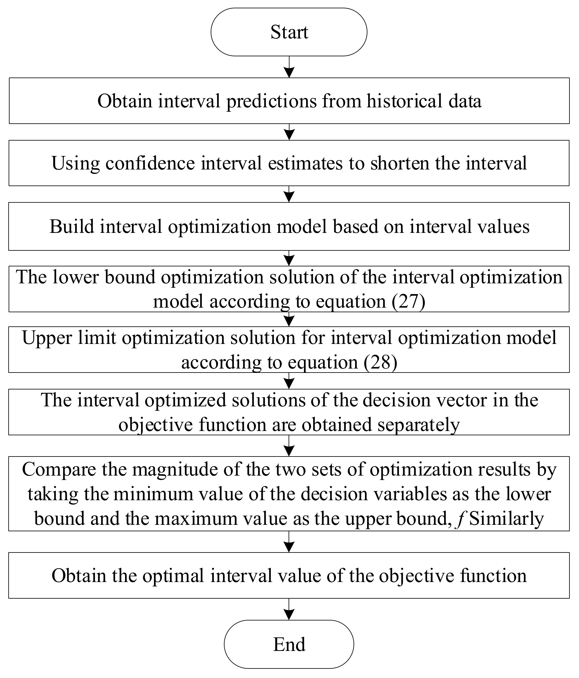
5.3. Interval Optimization Solving Steps

In this paper, wind power output and electric load are used as uncertainties to participate in reactive power optimization. The final interval solution takes the lowest total economy as the objective function and can be divided into an upper bound model and a lower bound model.

(1)

The lower bound model needs to get the optimistic value of the original model and the feasible domain needs to be as large as possible. The most optimistic scenario is that the wind power output is at its maximum and the grid load is at its minimum. The cost of energy purchase is significantly lower at this point, which further reduces the value of the objective function. The lower bound model is:

$$\begin{array}{l}\min f^{-}=c_{ploss}{\displaystyle {\displaystyle \sum }_{t\in T}}{I}_{ij,t}^2{R}_{ij}+c_{\text{buy}}{\displaystyle {\displaystyle \sum }_{t\in T}}{\displaystyle {\displaystyle \sum }_{k\in {\Omega }_g}}{P}_{k,t}^g\\ s.t{\displaystyle {\displaystyle \sum }_{j\in N\left(i\right)}}-g_{ij}{V}_{i,t}^2+V_{i,t}{V}_{j,t}\left(g_{ij}\cos {\theta }_{ij,t}+b_{ij}\sin {\theta }_{ij,t}\right)=[P_{i,t}^{\text{DG}}{]}^{+}+P_{i,t}^g-[P_{i,t}^{\text{load}}{]}^{-}\\ {\displaystyle {\displaystyle \sum }_{j\in N\left(i\right)}}{b}_{ij}{V}_{i,t}^2+V_{i,t}{V}_{j,t}\left(g_{ij}\sin {\theta }_{ij,t}-b_{ij}\cos {\theta }_{ij,t}\right)=Q_{i,t}^{\text{CB}}+Q_{i,t}^{\text{OLTC}}+Q_{i,t}^{\text{SVC}}+Q_{i,t}^g-{[Q_{i,t}^{\text{load}}]}^{-}\\ Eq.\left(6\right)-Eq.\left(20\right)\end{array}$$

(28)

(2)

The upper bound model needs to get the pessimistic value of the original model and the feasible domain needs to be as small as possible. The scenario with the minimum wind power output and maximum grid load is the most pessimistic scenario. The cost of energy purchase increases significantly at this point, further making the objective function value increase. In the planning model, the equations related to the uncertainty quantities are Equations (4) and (5). The upper bound model is:

$$\begin{array}{l}\min f^{+}=c_{ploss}{\displaystyle {\displaystyle \sum }_{t\in T}}{I}_{ij,t}^2{R}_{ij}+c_{\text{buy}}{\displaystyle {\displaystyle \sum }_{t\in T}}{\displaystyle {\displaystyle \sum }_{k\in {\Omega }_g}}{P}_{k,t}^g\\ s.t.{\displaystyle {\displaystyle \sum }_{j\in N\left(i\right)}}-g_{ij}{V}_{i,t}^2+V_{i,t}{V}_{j,t}\left(g_{ij}\cos {\theta }_{ij,t}+b_{ij}\sin {\theta }_{ij,t}\right)=[P_{i,t}^{\text{DG}}{]}^{+}+P_{i,t}^g-[P_{i,t}^{\text{load}}{]}^{+}\\ {\displaystyle {\displaystyle \sum }_{j\in N\left(i\right)}}{b}_{ij}{V}_{i,t}^2+V_{i,t}{V}_{j,t}\left(g_{ij}\sin {\theta }_{ij,t}-b_{ij}\cos {\theta }_{ij,t}\right)=Q_{i,t}^{\text{CB}}+Q_{i,t}^{\text{OLTC}}+Q_{i,t}^{\text{SVC}}+Q_{i,t}^g-{[Q_{i,t}^{\text{load}}]}^{+}\\ Eq.\left(6\right)-Eq.\left(20\right)\end{array}$$

(29)

(3)

Combining the optimal solutions of the upper bound model and the lower bound model, the global optimal interval solution is $f^{\pm }=[{\displaystyle \underset{¯}{f}},\overline{f}]$, where ${\displaystyle \underset{¯}{f}}=\min (f^{-},f^{+})$ and $\overline{f}=\max (f^{-},f^{+})$.

According to the above interval optimization model and solution method, the reactive power optimization model with source load uncertainty can be solved. The whole model is a MISOCP model. The decision variables are integer-type variables for the stall selection of CB and OLTC, and real-type variables for the output of SVC and DG. Among the constraints, the upper and lower bounds of voltage, current, and power are inequality constraints, and the active and reactive currents are equation constraints. Figure 1 shows the flow chart of linear interval programming.

6. Case Analysis

The system configuration is a computer (intel i7-5500, 2.40 GHz, 12 G), and the CPLEX algorithm package is called to solve the problem. The test case is the IEEE 33 node power distribution system [23]. The convergence gap of mixed-integer optimization is set to 0.1%. The calculation example contains three DGs connected to nodes 3, 17, and 28, respectively; three SVCs connected to nodes 5, 15, and 31, respectively; and two CBs joined to nodes 5 and 15, respectively, as shown in Figure 2.

Table 1. Parameters.

Types	Access Node	Quantity	Output Range
CB	5, 15	2	(0, 0.5) (MVar)
SVC	5, 15, 31	3	(−0.2, 0.4) (MVar)
DG	3, 17, 28	3	(0, 0.8) (MW)

shows the important parameters.

The DG model only considers the output of wind turbines. It is assumed that the units are in the same wind farm and the same external environment. The upper and lower limits of the wind power output are obtained for each moment based on historical data. The upper and lower limits are taken as interval quantities and substituted into the interval optimization model for corresponding solutions.

6.1. Static Optimal Power Flow Model

Table 2. Comparison of interval scheduling results under different fluctuation ranges.

Cases	Wind Power Fluctuation/%	Amplitude of Charge Fluctuation/%	Energy Purchase Cost/10,000 Yuan	Networks Loss Cost/10,000 Yuan	Total Cost/10,000 Yuan
1	0	0	3.070	0.029	3.099
2	± 10%	± 10%	(2.356, 3.808)	(0.023, 0.038)	(2.379, 3.846)
3	± 15%	± 10%	(2.266, 3.999)	(0.023, 0.039)	(2.289, 4.038)
4	± 10%	± 15%	(2.091, 4.086)	(0.021, 0.042)	(2.112, 4.128)
5	± 15%	± 15%	(2.002, 4.182)	(0.021, 0.043)	(2.023, 4.225)

shows a comparison of interval scheduling results under different fluctuation ranges. In order to reflect the impact of the degree of source–load uncertainty on the total cost, five different sets of source–load fluctuation ranges are set for comparison. The wind power fluctuation range is used to represent the degree of uncertainty at the source end, and the load fluctuation range represents the degree of uncertainty at the load end. The degree of uncertainty of source and load are both chosen from two values of ± 10% and ± 15%.

In Table 2, both the source and load fluctuations for Scenario 1 are zero. The optimization model is a deterministic model, and the predicted data are directly used as the actual values of the optimization model. No matter how the parameter values at both ends of the source load change, the target values of the deterministic model are between the interval solutions, which reflects the effectiveness of interval optimization. Comparing Case 2 and Case 3 shows that as the fluctuation of wind power increases, the fluctuation interval of the energy purchase cost increases. This in turn increases the radius of the total cost interval of the optimization model, further increasing the degree of uncertainty in the reactive power optimization and making the results more conservative. As the load volatility becomes larger, the operating environment becomes more hostile. With the same 5% increase in volatility, Case 4 is more conservative compared to the target interval solution of Case 3, and the total cost is taken to have a larger fluctuation range. In scenario 5, as the range of fluctuations of the source loads are all at their highest values, the resulting solution has the highest robustness.

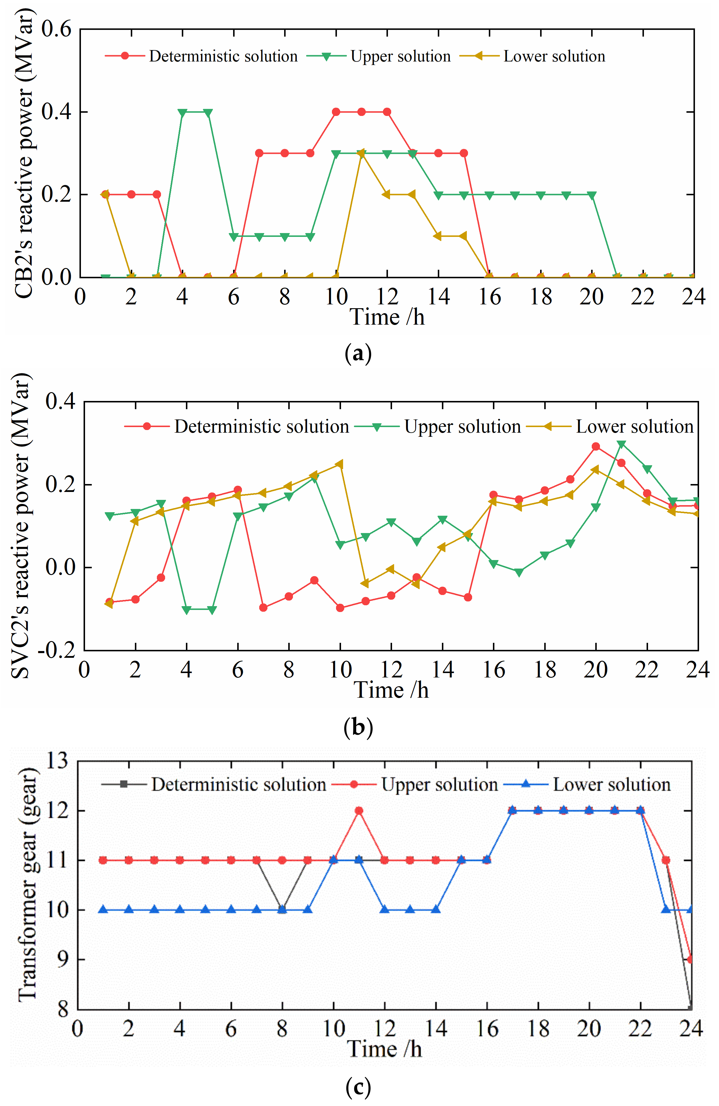
6.2. Deterministic Model Scheduling Results

In order to reflect the scientific nature of interval optimization, the optimization solutions of deterministic and uncertain models are compared, and the source load fluctuations are all taken as ± 10%. Since there are too many active management elements in the distribution network, the deterministic solution of CB2, SVC2, and OLTC and the interval optimization solution are selected for comparison, respectively. The interval optimized solutions are divided into interval upper bound solution and interval lower bound solution, and the specific comparison results are shown in Figure 3.

The interval solution is divided into an upper bound solution and a lower bound solution. The upper bound solution corresponds to the boundary case where the wind power output is the smallest and the load is the largest. The upper bound solution is the highest total economic cost due to the increase in energy purchase cost. The lower bound solution, on the contrary, corresponds to the boundary case where the wind power output is the largest and the load is the smallest.

In Figure 3a, the CB2 reactive power compensation is a discrete variable, and the CB2 reactive power compensation that determines the solution is mainly performed between 7:00 and 15:00. This time period is also the peak period of daily electricity consumption, and since the reactive power is insufficient, CB2 compensates by adjusting the gears. In the reactive power compensation volume of CB2, the total compensation volume of the upper boundary solution is significantly more than that of the lower boundary solution. This is because the upper boundary case has more load than the lower boundary case and requires more CB2 for reactive power compensation. In Figure 3b, the dynamic regulation of the transformer gears is basically the same. Due to the problem of varying load supply, where the stalls of the upper bound solution are all higher overall than the lower bound solution, the stalls of the solution are determined to be essentially the same as the upper bound solution in order to make the lowest total cost. In Figure 3c, the value of reactive power compensation of SVC2 varies in magnitude and is a continuous-type variable. In the time period when the load demand is high, the difference between the upper bound solution and the lower bound solution increases significantly. It means that the amount of reactive power compensation still depends on the actual load demand, and the volatility of the source load increases the uncertainty of the cost. All the above phenomena indicate that interval-optimized reactive power compensation is mainly supplied for different time periods of load demand. In summary, the more conservative the scheme, the larger the interval range of the total cost.

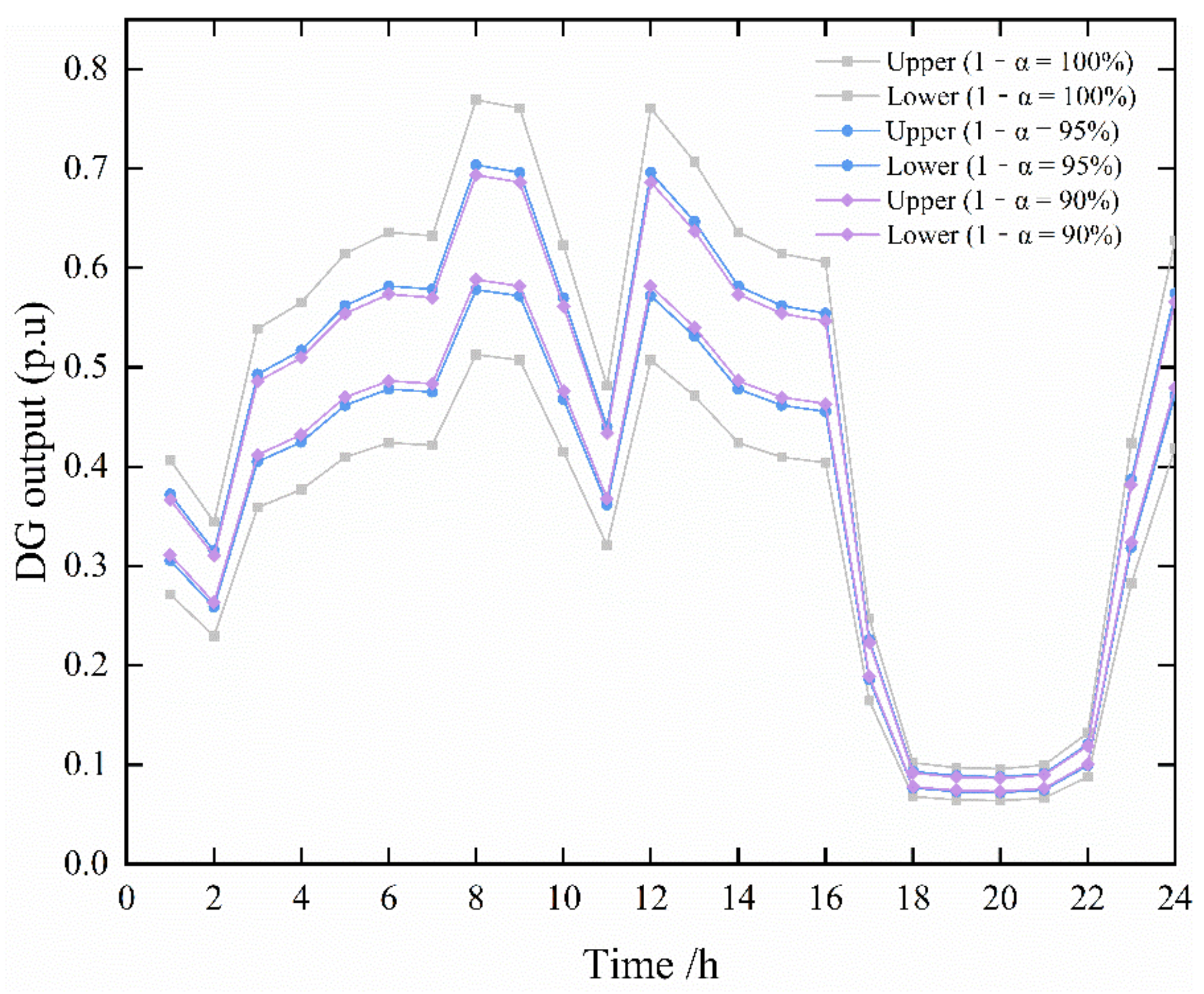
6.3. Effect of Different Confidence

Figure 4 shows the load intervals at different confidence levels. The level of confidence level reflects the requirement of the scheduling decision on the reliability of system operation, and the fluctuation of wind power and load is set to ± 15%. To analyze the impact of different confidence levels on the scheduling scheme, the power interval variables are extracted with confidence levels of 100%, 95%, and 90%, respectively.

When the confidence levels are 100% and 95%, respectively, there is a significant difference in terms of the range of loading intervals, although the difference is only 5% in terms of confidence level. When the confidence level is taken as 100%, the comprehensiveness of the extracted intervals can be guaranteed. However, there are some regions with low probability of occurrence in the interval range, which can easily interfere with the selection of the scheme in practical applications.

Table 3. Comparison of schemes under different confidence levels.

Confidence $1-\mathit{\alpha }$/%	Energy Purchase Cost/10,000 Yuan	Networks Loss Cost/10,000 Yuan	Total Cost/10,000 Yuan
100	(2.002, 4.182)	(0.021, 0.043)	(2.023, 4.225)
95	(2.370, 3.793)	(0.023, 0.038)	(2.393, 3.831)
90	(2.482, 3.676)	(0.024, 0.036)	(2.506, 3.712)
80	(2.555, 3.600)	(0.025, 0.035)	(2.580, 3.635)

shows the scheduling results of the optimal scheme with different confidence intervals. The power fluctuation range is large when the confidence interval is taken as 100%, and all uncertainty factors are considered. The interval difference is significantly larger than the other schemes. The scheduling scheme tends to be conservative, which inevitably leads to resource waste, and thus economic losses. The solution obtained under the low confidence interval has a smaller interval difference, and the solution is more accurate, which can reduce part of the economic loss. On the other hand, the program allows less flexibility due to the reduced confidence level. In this way, power fluctuations outside the interval range may occur, leading to unplanned power adjustments. Therefore, in practical applications, it is necessary to consider reliability and economy and select the appropriate confidence level to optimize system operation.

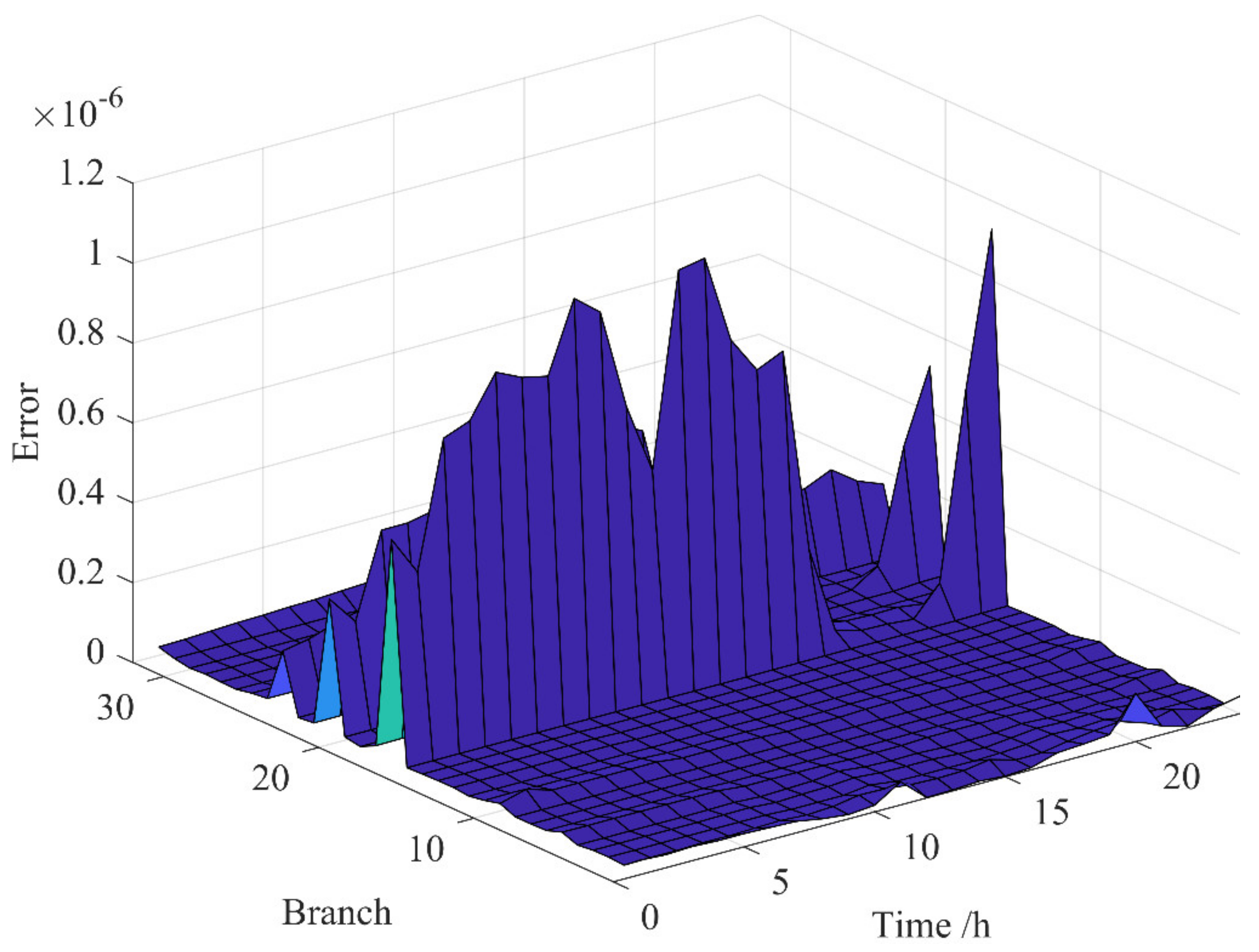
6.4. Effectiveness Analysis of Second-Order Cone Relaxation

Figure 5 shows the error of each branch under different time periods. To improve the solution’s efficiency, the reactive power optimization model is relaxed by the second-order cone. We analyze the effectiveness of the second-order cone after relaxation. The error after the second-order cone relaxation satisfies the requirements of the operation plan, which meets the corresponding requirements in actual engineering.

Table 4. Comparison of solving speed under different algorithms.

Model	Algorithm	Time
MISOCP	CPLEX	67.63 s
MINLP	Bonmin	Infeasible

shows the comparison of the solution speeds under different algorithms. The model after the second-order cone relaxation is a mixed-integer, second-order cone programming program (MISOCP), instead of being transformed into a mixed-integer, non-linear program (MINLP). The two models are solved by CPLEX and Bonmin solvers, respectively. Table 3 shows that the MINLP is an unsolvable problem, which verifies the superiority of the method proposed in this paper.

7. Conclusions

For the uncertainty of new energy output, this paper proposes a distribution network reactive power optimization model based on interval optimization. The model has the following characteristics:

(1)

The model is an optimal dynamic power flow model for the active distribution network, taking into account a variety of active management elements in the distribution network. The generation method of the model can better adapt to the actual changes in load demand at various times of the day.

(2)

Confidence interval estimation methods can reduce the range of interval solutions. They can improve the accuracy of the interval solution and avoid economic loss with high probability.

(3)

The interval optimization method can make the generation solution space encompass all possible cases and can adapt to the case of fluctuations in uncertain variables. It ensures the reliability of power supply and improves the power quality.

(4)

The second-order cone relaxation technique can improve the efficiency of model solving. It ensures that the error of the generated solution is within the allowed range and meets the needs of practical engineering.

The reactive power optimization model established in this paper is an optimal dynamic power flow problem. The next step will focus on further consideration of the demand response characteristics in the distribution network.

References

1. Muhammad, M.A.; Mokhlis, H.; Naidu, K.; Amin, A.; Franco, J.F.; Othman, M. Distribution Network Planning Enhancement via Network Reconfiguration and DG Integration Using Dataset Approach and Water Cycle Algorithm. J. Mod. Power Syst. Clean Energy 2020, 8, 86–93. [Google Scholar] [CrossRef]
2. Kumar, S.; Sarita, K.; Vardhan, A.S.S.; Elavarasan, R.M.; Saket, R.K.; Das, N. Reliability Assessment of Wind-Solar PV Integrated Distribution System Using Electrical Loss Minimization Technique. Energies 2020, 13, 5631. [Google Scholar] [CrossRef]
3. Mohamed, M.A.-E.-H.; Ali, Z.M.; Ahmed, M.; Al-Gahtani, S.F. Energy Saving Maximization of Balanced and Unbalanced Distribution Power Systems via Network Reconfiguration and Optimum Capacitor Allocation Using a Hybrid Metaheuristic Algorithm. Energies 2021, 14, 3205. [Google Scholar] [CrossRef]
4. Romero, R.; Franco, J.F.; Leão, F.B.; Rider, M.J.; de Souza, E.S. A New Mathematical Model for the Restoration Problem in Balanced Radial Distribution Systems. IEEE Trans. Power Syst. 2016, 31, 1259–1268. [Google Scholar] [CrossRef] [Green Version]
5. Song, C.; Luo, Q.; Shi, F. Genetic Algorithms for Optimization of Complex Nonlinear System. In Proceedings of the 2008 International Conference on Computer Science and Software Engineering, Wuhan, China, 12–14 December 2008; Volume 1, pp. 378–381. [Google Scholar]
6. Kennedy, J.; Eberhart, R. Particle Swarm Optimization. In Proceedings of the Proceedings of ICNN’95—International Conference on Neural Networks, Perth, WA, Australia, 27 November–1 December 1995; Volume 4, pp. 1942–1948. [Google Scholar]
7. Tran, T.T.; Truong, K.H.; Vo, D.N. Stochastic Fractal Search Algorithm for Reconfiguration of Distribution Networks with Distributed Generations. Ain Shams Eng. J. 2020, 11, 389–407. [Google Scholar] [CrossRef]
8. Ivanov, O.; Neagu, B.-C.; Grigoras, G.; Gavrilas, M. Optimal Capacitor Bank Allocation in Electricity Distribution Networks Using Metaheuristic Algorithms. Energies 2019, 12, 4239. [Google Scholar] [CrossRef] [Green Version]
9. Wang, J.; Chen, H. BSAS: Beetle Swarm Antennae Search Algorithm for Optimization Problems. arXiv 2018, arXiv:1807.10470. [Google Scholar]
10. Farivar, M.; Low, S.H. Branch Flow Model: Relaxations and Convexification—Part I. IEEE Trans. Power Syst. 2013, 28, 2554–2564. [Google Scholar] [CrossRef]
11. Farivar, M.; Low, S.H. Branch Flow Model: Relaxations and Convexification—Part II. IEEE Trans. Power Syst. 2013, 28, 2565–2572. [Google Scholar] [CrossRef]
12. Scarabaggio, P.; Grammatico, S.; Carli, R.; Dotoli, M. Distributed Demand Side Management With Stochastic Wind Power Forecasting. IEEE Trans. Control Syst. Technol. 2022, 30, 97–112. [Google Scholar] [CrossRef]
13. Zhao, C.; Guan, Y. Data-Driven Stochastic Unit Commitment for Integrating Wind Generation. IEEE Trans. Power Syst. 2016, 31, 2587–2596. [Google Scholar] [CrossRef]
14. Roustaei, M.; Niknam, T.; Salari, S.; Chabok, H.; Sheikh, M.; Kavousi-Fard, A.; Aghaei, J. A Scenario-Based Approach for the Design of Smart Energy and Water Hub. Energy 2020, 195, 116931. [Google Scholar] [CrossRef]
15. Duan, C.; Jiang, L.; Fang, W.; Liu, J.; Liu, S. Data-Driven Distributionally Robust Energy-Reserve-Storage Dispatch. IEEE Trans. Ind. Inform. 2018, 14, 2826–2836. [Google Scholar] [CrossRef] [Green Version]
16. Wang, C.; Jiao, B.; Guo, L.; Tian, Z.; Niu, J.; Li, S. Robust Scheduling of Building Energy System under Uncertainty. Appl. Energy 2016, 167, 366–376. [Google Scholar] [CrossRef]
17. Wang, Y.; Xia, Q.; Kang, C. Unit Commitment With Volatile Node Injections by Using Interval Optimization. IEEE Trans. Power Syst. 2011, 26, 1705–1713. [Google Scholar] [CrossRef]
18. Bai, L.; Li, F.; Cui, H.; Jiang, T.; Sun, H.; Zhu, J. Interval Optimization Based Operating Strategy for Gas-Electricity Integrated Energy Systems Considering Demand Response and Wind Uncertainty. Appl. Energy 2016, 167, 270–279. [Google Scholar] [CrossRef] [Green Version]
19. Wu, L.; Shahidehpour, M.; Li, Z. Comparison of Scenario-Based and Interval Optimization Approaches to Stochastic SCUC. IEEE Trans. Power Syst. 2012, 27, 913–921. [Google Scholar] [CrossRef]
20. Fang, X.; Cui, H.; Yuan, H.; Tan, J.; Jiang, T. Distributionally-Robust Chance Constrained and Interval Optimization for Integrated Electricity and Natural Gas Systems Optimal Power Flow with Wind Uncertainties. Appl. Energy 2019, 252, 113420. [Google Scholar] [CrossRef]
21. Lei, Y.; Wang, D.; Jia, H.; Chen, J.; Li, J.; Song, Y.; Li, J. Multi-Objective Stochastic Expansion Planning Based on Multi-Dimensional Correlation Scenario Generation Method for Regional Integrated Energy System Integrated Renewable Energy. Appl. Energy 2020, 276, 115395. [Google Scholar] [CrossRef]
22. Zheng, X.; Qiu, Y.; Zhan, X.; Zhu, X.; Keirstead, J.; Shah, N.; Zhao, Y. Optimization Based Planning of Urban Energy Systems: Retrofitting a Chinese Industrial Park as a Case-Study. Energy 2017, 139, 31–41. [Google Scholar] [CrossRef]
23. Rugthaicharoencheep, N.; Sirisumrannukul, S. Optimal Feeder Reconfiguration with Distributed Generators in Distribution System by Fuzzy Multiobjective and Tabu Search. In Proceedings of the 2009 International Conference on Sustainable Power Generation and Supply, Nanjing, China, 6–7 April 2009; pp. 1–7. [Google Scholar]
Figure 1. Flow chart of linear interval programming.
Energies 15 02235 g001
Figure 2. IEEE 33 bus system.
Energies 15 02235 g002
Figure 3. Comparison of interval-optimized solutions and deterministic solutions: (a) Comparison of reactive power compensation of CB2; (b) Comparison of reactive power compensation of SVC2. (c) Comparison of transformer gears.
Energies 15 02235 g003
Figure 4. DG output interval forecast.
Energies 15 02235 g004
Figure 5. The error of each branch at different times.
Energies 15 02235 g005