Resilience-Oriented Framework for Microgrid Planning in Distribution Systems

Abstract

Recently, it has been suggested that microgrids (MGs) can improve the resilience of distribution systems. However, predictions about future faults are uncertain. This makes calculating the exact value of the benefits of system resilience enhancement close to impossible at the time of MG planning. Therefore, this paper proposes a framework for MG planning, which focuses on resilience estimation. To consider the uncertainties of future failure events, the proposed method for estimating the resilience utilized the Monte Carlo simulation. In addition, an optimal scenario was estimated using a cost–benefit analysis and constraints on the expected value of resilience enhancement. In the case study, an actual MG installation at D-university was evaluated to obtain the optimal MG planning scenario. The results show that the capacity and installation locations of the distributed generators (DGs) impact the resilience enhancement. The proposed method can effectively derive the optimal MG planning scenario by evaluating the possibility of future operations based on the segmentation of both the system configuration and type of DG to improve the resilience of distribution systems.

1. Introduction

Power system resiliency is defined as the ability to prepare for, adapt to, and recover rapidly from disruptive events [1]; it considers high-impact low-frequency events such as natural disasters and deliberate attacks [2]. Even a single occurrence of an event such as a natural disaster can cause critical problems in the power system. However, it is impossible to reduce the intensity of a natural disaster [3]. For this reason, the resilience enhancement of power systems is being increasingly researched.

In previous studies on resilience assessment, frameworks for resilience assessment with various goals were proposed to respond to natural disasters [4], including a specific disaster (typhoon) [5]. Moreover, the importance of a resilience metric for power systems has been highlighted [6]. Especially, rapid recovery is considered the most important feature of a resilience metric [7]. In this regard, microgrids (MGs), which operate the distributed generators (DGs), have been projected as a potential solution for supporting the rapid recovery of the resilience of a distribution system [8].

Existing studies on MG planning based on economic feasibility have considered the problem of DG sizing [9,10]. However, MG planning considering the resilience must involve the assessment process of the resilience of a distribution system to disruptive events. Hence, not only long-term planning but also short-term planning and operations should be reflected in the framework for MG planning [11].

In previous studies on resilience-oriented operation with MG, the categorization of DGs and sectionalization of systems were established as methods for rapidly recovering from failures [12]. An optimization method based on the maximum allowable load loss was proposed for minimizing the investment costs [13].

In addition, a three-level model based on the multi-objective optimization problem was proposed in a previous study on resilience-oriented long-term planning with MG [14]. In the model, load profile uncertainty and some contingencies were considered, and the results proved a trade-off relationship between cost and resilience. In another study, multiple objective functions that maximize the critical load and minimize the capacity of dispatchable DGs were proposed for cost-effective MG planning [15]. A framework that incorporated resilience was developed for the economic assessment of MGs [16]. The cost–benefit analysis (CBA) in this framework comprised three steps and provided benefits of enhancement in the resilience and reliability through MG installation.

As mentioned in previous studies, to realize the success of long-term planning efforts, including MG installation, it is crucial to establish a framework that integrates various methods, such as that for system configuration, with the measurement criteria including that for the critical load. Nevertheless, owing to the uncertainty of events (type and intensity of disasters, number and location of failures, and time of failure occurrence and repair for each system), the uncertainty of various contingencies rather than the load profile uncertainty should be preferentially reviewed in the framework.

To address the problem of power distribution system reinforcement while avoiding the above issues, the resilience considering uncertainties was probabilistically evaluated using a Monte Carlo simulation (MCS) and the results were used as constraints for feasibility analysis [17]. To apply these prior studies to a real-world system, a more intuitive presentation of the effect of resilience enhancement is required for the system operator, and various types of components, such as DGs, should be applied in the system.

Thus, this study proposes a resilience-oriented framework for MG planning. The framework consists of a probabilistic resilience estimation method, expected value of resilience enhancement (EoRE) estimation method, and CBA method. In the process, the post-contingency uncertainties are considered, and the various output characteristics of the DGs are reflected. As a case study, the MG planning of D-university was conducted using the proposed framework. The proposed method provides both the EoRE and CBA results, enabling the system operators in charge of MG planning or the MG operators to make an informed and reasonable judgment of the amount of resilience enhancement that should be set as a priority.

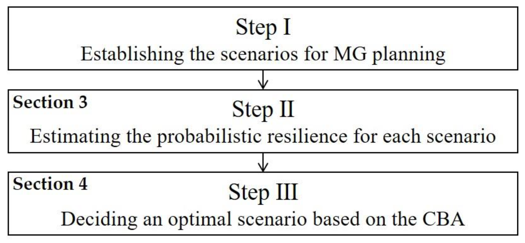
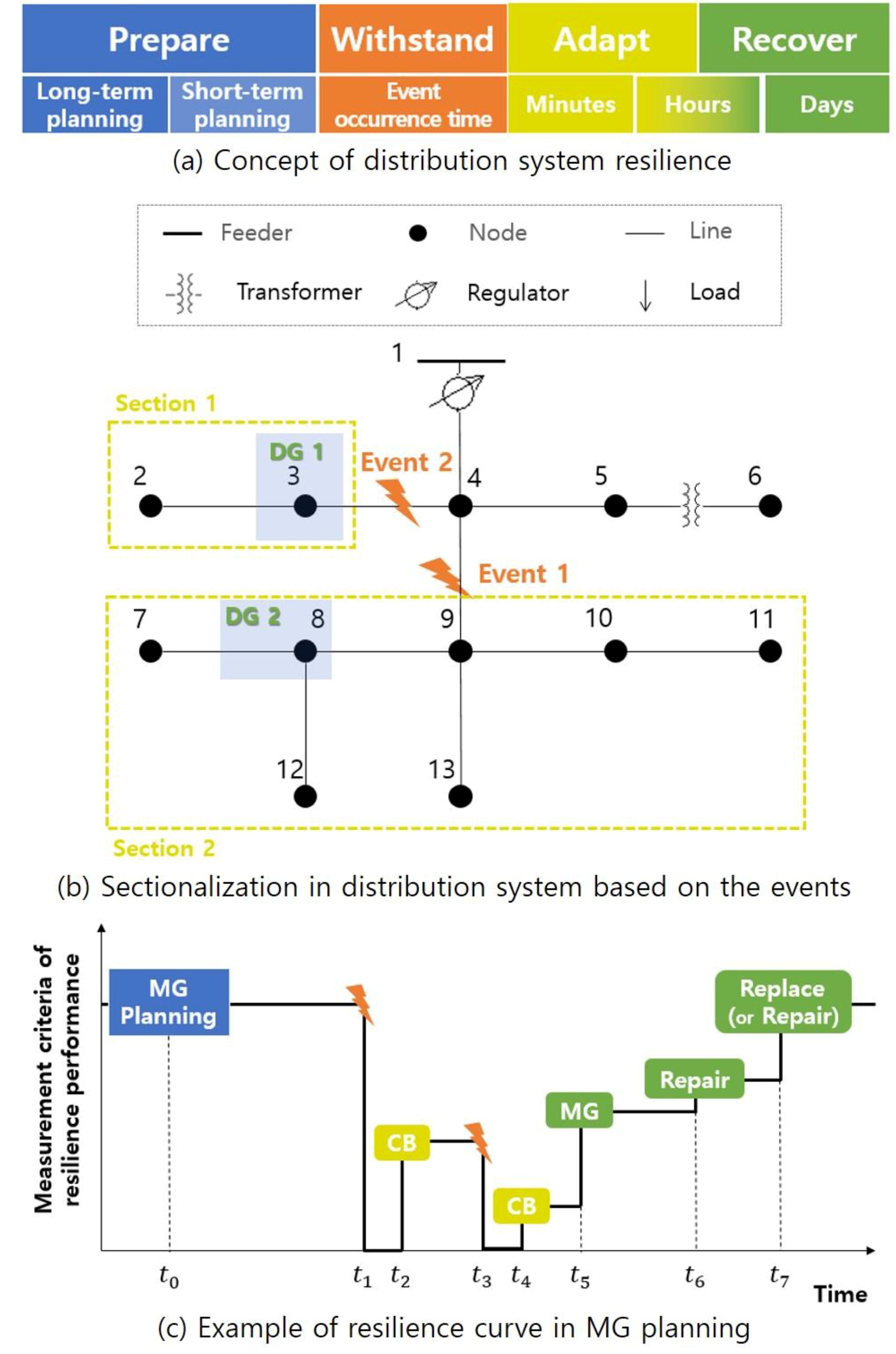
2. Framework of Microgrid Planning

MG planning is generally conducted based on the economic evaluation using load analysis, power generation forecasting, and system configuration [9,10]. In the case of MG planning considering the reliability, formulaic indices such as system average interruption duration index (SAIDI) and loss of load expectation (LOLE) are used [18]. In addition, the economic value of the reliability is estimated in terms of the outage costs per year according to the type of customers using the customer damage function [19]. However, owing to the uncertainty of contingencies in the future, determining a single value that reflects the benefit of resilience enhancement in MG planning is difficult. Furthermore, frameworks for MG planning including the generalized resilience indices are under development in various viewpoints.

With the objective of reducing the investment required for resilience enhancement in a contingency, this paper proposes a framework for MG planning, which comprises three steps, as shown in Figure 1.

In step I, the various scenarios are established according to the purpose of the MG planner. In this step, the capacity as well as the type and location of the DG should be considered for each scenario, not only to maximize the economic benefits but also to improve the resilience of the system. The specific information of the established scenario is used to estimate the resilience enhancement in step II and cost-effectiveness in step III. In step II, the probabilistic evaluation of the resilience is conducted. In step III, the results of the probabilistic resilience are utilized to select the scenarios that satisfy the resilience constraints, and the optimal scenario is provided based on the commonly used CBA.

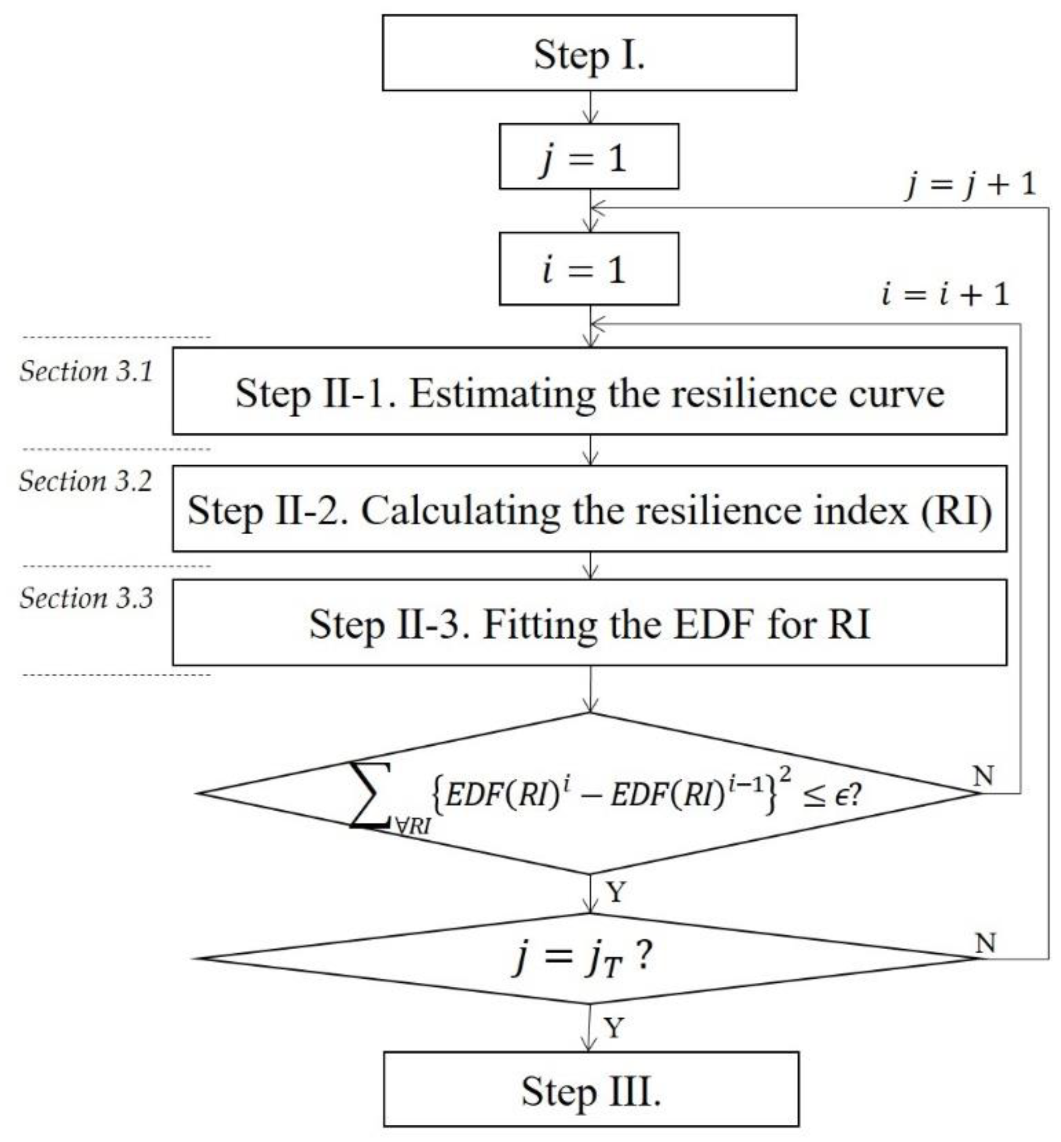
3. Estimation Method for Probabilistic Resilience

The probabilistic estimation of resilience, mentioned in step II of Figure 1, is illustrated in Figure 2 [17]. This method utilized MCS to derive the results of the probabilistic resilience, considering the post-contingency uncertainty in the development phase of MG planning. MCS is an inferential statistical technique that estimates an unknown value based on several simulations. It is used to derive a specific numerical value or probability distribution through the repeated random sampling of random variables. This study sets several random variables (e.g., location and occurrence time of failure and recovery time) for the event uncertainties to derive a probability distribution of the system’s resilience performance.

As depicted in Figure 2, the probabilistic estimation process of resilience comprises three sub-steps of step II. In particular, the resilience curve is estimated in step II-1, considering the fault and recovery information for post-contingency. Thereafter, the resilience index (RI) is calculated in step II-2 for resiliency evaluation, and the RI results are fitted to the empirical distribution function (EDF) in step II-3. The MCS is completed when the EDF(RI) satisfies the convergence range ($ϵ$). The MCS was applied to all the MG planning scenarios ($j_T$).

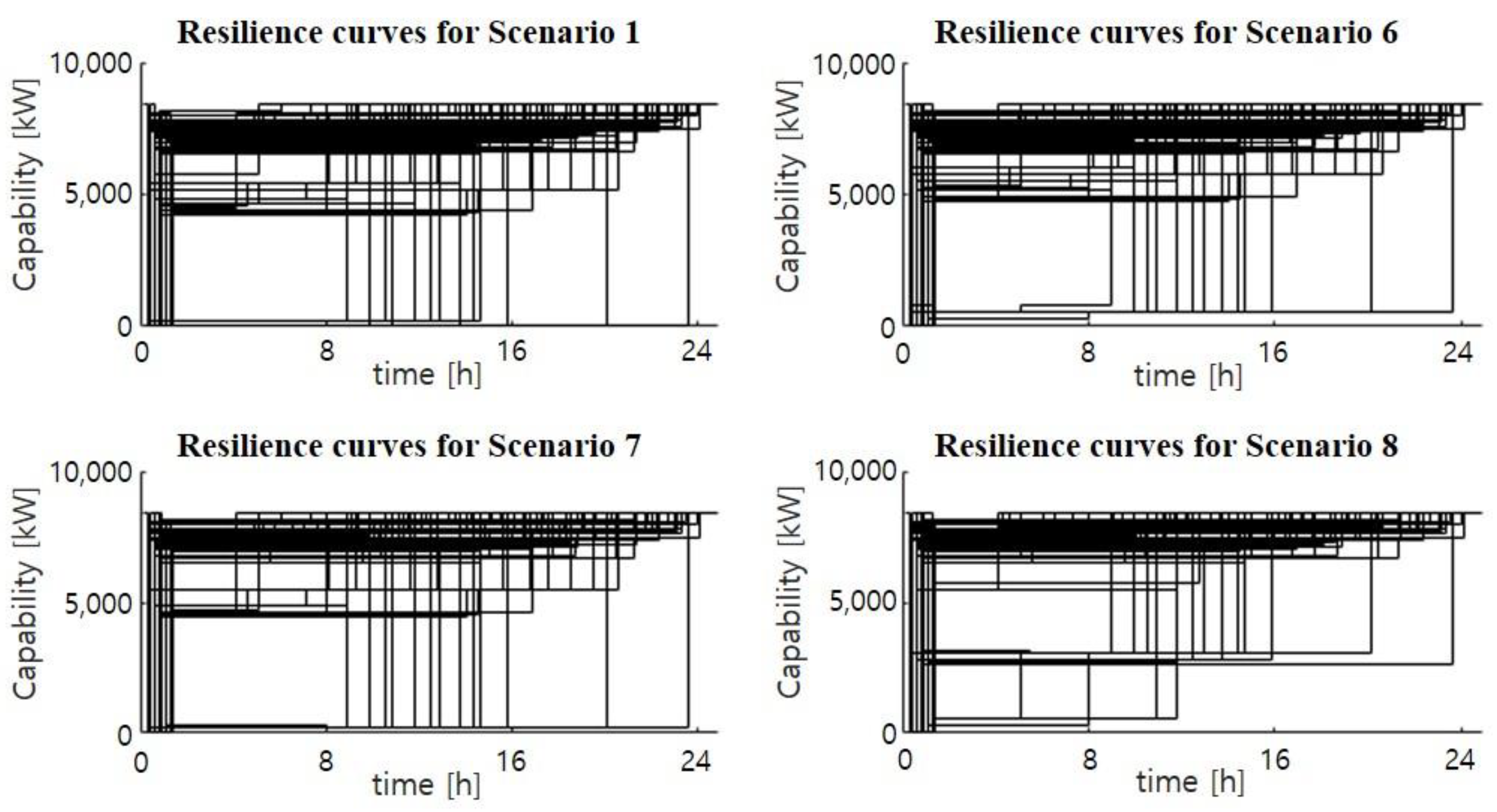
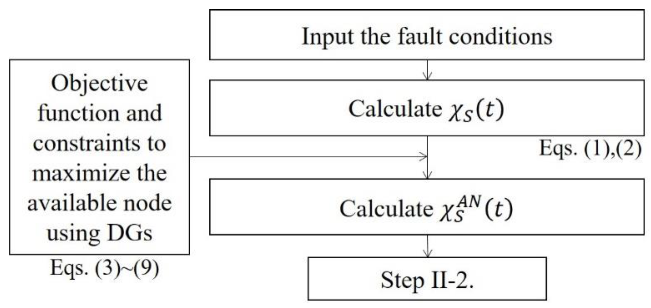
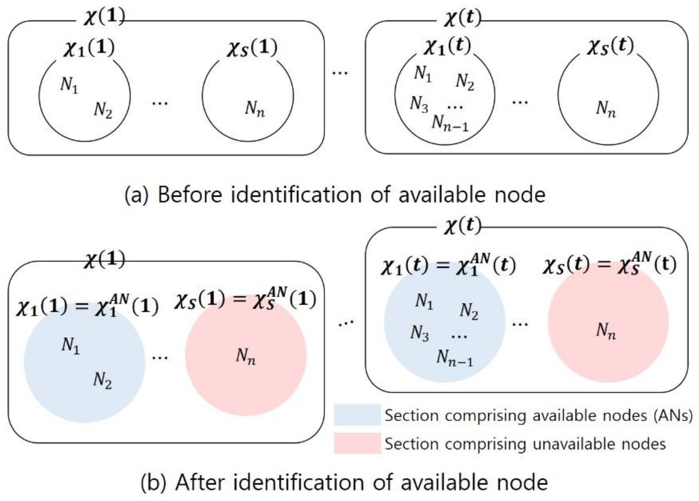
3.1. Estimating the Resilience Curve (Step II-1)

In this study, the resilience curve was defined as the “time-varying performance of the system.” An example of the estimation method used to establish the resilience curve is shown in Figure 3.

Figure 3a specifically explains the concept of distribution system resilience. Figure 3b illustrates an example to relate the fault situation in a distribution system to the resilience concept. In Figure 3b, the locations of the DGs were set to nodes 3 and 8 in the preparation process of long-term planning, and the failure locations were assumed to be lines 4–9 and 3–4 in the withstand process. In the adapt process, the system was sectionalized via circuit breakers (CBs). DGs were contributed to supply power to each section. Figure 3c describes the resilience curve for Figure 3b. The diagram shows the system’s resilience performance at each of the following time points: the moment of equipment failure at the time of the event ($t_1,t_3$), the moment when the system is sectionalized via a CB ($t_2,t_4$), the moment when power is supplied using the DG in each section ($t_5$), and the moment when the equipment is restored through repair or replacement ($t_6,t_7$).

To estimate the resilience curve in this manner, the sectionalization of the system in event situations and a method to derive the nodes where power can be supplied using a DG are needed. This study proposes the resilience curve estimation process shown in Figure 4.

In this study, the topology $\chi$ of a particular distribution system is defined as a set of nodes expressed in Equation (1):

$$\left\{N_1,N_2,\dots ,N_n\right\}\in \chi ,$$

(1)

where $N_n$ represents the nth node, and the pre-failure topology $\chi$ of a single power system is a set that comprises all the nodes as elements.

When the events occur in a particular distribution system, the sections are separated via CBs and can be expressed as a subset of the topology $\chi$ as follows:

$${\chi }_S\subset \chi ,$$

(2)

where ${\chi }_S$ represents the sth section of the topology separated by an event.

In Figure 4, the fault condition consists of the number, type, and location of the failed equipment and the failure and recovery time for each piece of equipment. Based on this condition, the nodes ($N_n$) included in each section are organized according to time (t), as depicted in Figure 5a.

As depicted in Figure 5, the nodes ($N_n$) in each section (${\chi }_S\left(t\right)$) are physically connected but power outages may occur owing to the loss of power supply. This means that the available nodes (ANs) in each section ${\chi }_S\left(t\right)$ along with the time-variant section ${\chi }_S^{AN}\left(t\right)$ comprising the ANs, shown in Figure 5b, must be determined.

Thus, the objective function was applied as expressed in Equation (3) with the constraints expressed in Equations (4)–(9). The proposed method evaluates the adequacy of the capability (available capacity) by using the peak load for each node and the capacity of each DG [20]. These equations are equally applied to each ${\chi }_S\left(t\right)$ to select the optimal ${\chi }_S^{AN}\left(t\right)$ containing the ANs.

$$\max {\displaystyle \sum }_{N\in AN}{R}_N^{\xi }$$

(3)

$${\displaystyle \sum }_{N\in AN}{L}_N\le P_{feeder}+{\displaystyle \sum }_{\forall DG}{P}_{DG}$$

(4)

$${\displaystyle \sum }_{\forall DG}{P}_{DG}={\displaystyle \sum }_{\forall CDG}{P}_{CDG}+{\displaystyle \sum }_{\forall NDG}{P}_{NDG}+{\displaystyle \sum }_{\forall ESS}{P}_{ESS}$$

(5)

$$P_{NDG}=\left\{\begin{array}{c}{\omega }_{NDG}·P_{NDG}\hspace{0.33em}\hspace{0.33em}if E_{NDG}\le E_{ESS}\\ 0\hspace{0.33em}\hspace{0.33em}\hspace{0.33em}\hspace{0.33em}otherwise\end{array}\right.$$

(6)

$$E_{NDG}={\displaystyle \sum }_{\forall NDG}{\omega }_{NDG}·P_{NDG}·T$$

(7)

$${\omega }_{NDG}=\frac{a{t}_{NDG}}{24}$$

(8)

$$P_{ESS}=\left\{\begin{array}{c}\frac{E_{ESS}}{T} if \frac{E_{ESS}}{T}\le P_{PCS}\\ P_{PCS} otherwise\end{array}\right.$$

(9)

Equation (3) represents the objective function used to determine the AN value that maximizes the sum of the resilience performance (${\displaystyle \sum }_{N\in AN}{R}_N^{\xi }$) for ${\chi }_S^{AN}\left(t\right)$. In this case, $\xi$ represents the performance metrics, which can be applied specifically according to the measurement criteria that the system operator intends to evaluate, such as the peak load of the AN, number of customers, and number of critical customers of AN.

In Equation (4), ${\displaystyle \sum }_{N\in AN}{L}_N$ is the sum of the peak loads of the ANs and must be less than or equal to the sum of the capabilities ($P_{feeder}+{\displaystyle \sum }_{\forall DG}{P}_{DG}$) of the feeder and DG.

In Equation (4), if only the non-controllable DGs (NDGs) dependent on the natural environment are present in a specific section, e.g., photovoltaic (PV) and wind turbines (WT), they can cause an interruption in future operations. Equation (5) expresses the output characteristics of a DG divided into NDG and controllable DG (CDG), and the energy storage system (ESS) is included separately as it can charge as well as discharge power.

For Equation (6), the capability of each NDG ($P_{NDG}$) is calculated using ${\omega }_{NDG}·P_{NDG}$ when the energy produced from NDG ($E_{NDG}$) [kWh] can be controlled using $E_{ESS}$ [kWh] during the time between the occurrence of disaster and recovery (T). However, if this is not feasible, $P_{NDG}$ is calculated as “0,” assuming that curtailment occurs by manipulating the inverter for each NDG.

Equation (7) depicts the evaluation of $E_{NDG}$ used in Equation (6). As expressed, $E_{NDG}$ can be calculated by using the weighting factor (${\omega }_{NDG}$) and time of occurrence of failure (T), where ${\omega }_{NDG}$ is calculated using the average daily production time for NDG ($a{t}_{NDG}$), as shown in Equation (8). In Equation (9), $P_{ESS}$ is used when the dischargeable capacity over time for ESS ($E_{ESS}/T$) is less than the power conversion system capacity of ESS ($P_{PCS}$). Otherwise, $P_{PCS}$ is used.

The sections satisfying Equations (3)–(9) are represented as ${\chi }_S^{AN}\left(t\right)$. Equation (10) represents the time-varying performance of the distribution system [17].

$$R_T^{\xi }\left(t\right)={\displaystyle \sum }_{N_n\in ANs}{R}_N^{\xi }\left(t\right)$$

(10)

$R_T^{\xi }\left(t\right)$ from Equation (10) represents the time-varying performance of the system, whereas $R_N^{\xi }\left(t\right)$ represents the time-varying performance of each node.

3.2. Calculating the Resilience Index (Step II-2)

The resilience index ($R{I}^{\xi }$) used in this study is expressed in Equation (11) [21].

$$R{I}^{\xi }=\frac{{{\displaystyle \int }}_{}^T{R}_T^{\xi }\left(t\right)}{{{\displaystyle \int }}_{}^T{R}_{T0}^{\xi }\left(t\right)}$$

(11)

In Equation (11), $R_T^{\xi }\left(t\right)$ and $R_{T0}^{\xi }\left(t\right)$ represent the resilience curve assuming that a failure occurred and did not occur, respectively.

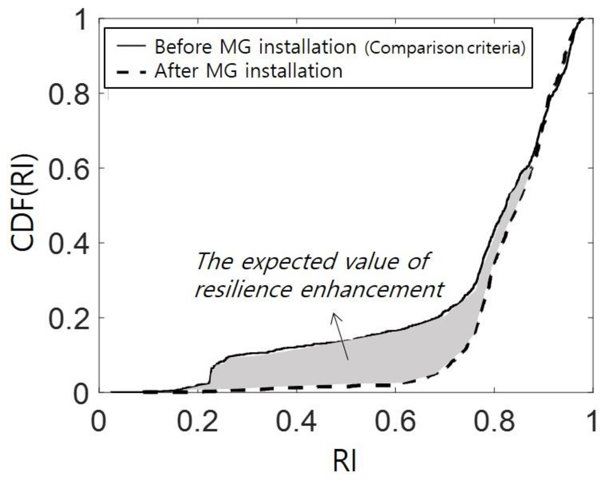
3.3. Fitting EDF for RI (Step II-3)

As mentioned above, $R{I}^{\xi }$ comprises the various sets ($R{I}^{\xi ,j}$) expressed in Equation (12) according to the criteria for performance measurement and the scenarios of MG planning.

$$R{I}^{\xi ,j}=\left\{R{I}^{1,\xi ,j},\dots ,R{I}^{i,\xi ,j}\right\}$$

(12)

The set of RI is fitted as an EDF. This study expresses the probability density function (PDF) as $PDF\left(R{I}^{\xi ,j}\right)$. The cumulative distribution function (CDF) is calculated as shown in Equation (13) [17,22].

$$CDF\left(R{I}^{\xi ,j}\right)={{\displaystyle \int }}_0^{R{I}^{\xi ,j}}PDF\left(R{I}^{\xi ,j}\right)dR{I}^{\xi ,j}$$

(13)

4. Optimal MG Planning Considering Resilience Based on Cost–Benefit Analysis

To determine the optimal MG planning scenario, this section presents the CBA and resilience constraints. As this study considers the resilience of the distribution system during the MG planning process, the costs and benefits in the CBA are applied from the perspectives of the utility and MG operators.

4.1. Cost–Benefit Analysis

In this study, the method for determining the optimal MG planning scenario is de-scribed based on the benefit–cost (B–C) ratio among the various methodologies for CBA. Generally, there is an investment value of B–C ratios greater than or equal to 1, and there is a decreased investment value when the B–C ratio is less than 1.

In this study, the scenario achieves the maximum B–C ratio, which is expressed as Equation (14).

$$\max \left(\frac{B_T^j}{C_T^j}\right)$$

(14)

The elements of B and C in Equation (14) are expressed in Equations (15)–(16); these are estimated from parameters such as life cycle and power output forecasting for each DG [9,10].

$$B_T^j=B_{MG}^j+B_{Utility}^j+B_{enviroment}^j$$

(15)

$$C_T^j=C_{MG}^j+C_{Utility}^j$$

(16)

In Equation (15), the benefit (B) is categorized into the benefit from the perspective of the environment and those from the perspectives of the MG operators and utilities, and the calculations for each benefit category are expressed in Equations (17)–(19). On the contrary, the cost (C) presented in Equation (16) is divided into the costs for MG operators and utilities and is subdivided as shown in Equations (20) and (21).

$$B_{MG}^j=B_{ES}^j+B_{sell}^j$$

(17)

$$B_{Utility}^j=B_{AC}^j+B_{AE}^j$$

(18)

$$B_{enviroment}^j=E_{DG}^j·e·U{C}_{CO2}$$

(19)

$$C_{MG}^j=C_{capital}^j+C_{O\&M}^j+C_{DG.fuel}^j$$

(20)

$$C_{Utility}^j=C_{RF}^j+C_{buy}^j$$

(21)

4.2. Resilience Constraint

As the constraints of power balancing and DG capacity were considered during resilience calculation, this section focuses on the resilience constraints.

In this study, the effect of resilience enhancement through MG installation is calculated as in Equation (22) below:

$$EoR{E}^{\xi ,j}=E\left[R{I}^{\xi ,j}\right]-E\left[R{I}^{\xi ,Ref.}\right],$$

(22)

where EoRE denotes the expected value of the resilience enhancement, and $E\left[R{I}^{\xi ,j}\right]$ indicates the expected value of the RI for the respective MG installation scenarios. $E\left[R{I}^{\xi ,Ref.}\right]$ denotes the comparison criteria for $E\left[R{I}^{\xi ,j}\right]$, which can be set considering the objectives, e.g., prior to MG implementation or increased DG capacity for MG. Using the CDF(RI) that was derived above, EoRE can be calculated as shown in Equation (23) below [23,24].

$$EoR{E}^{\xi ,j}={{\displaystyle \int }}_0^1\left[CD{F}_1\left(RI\right)-CD{F}_2\left(RI\right)\right]dRI$$

(23)

In Equation (23), $CD{F}_1\left(RI\right)$ denotes ($CDF\left(R{I}^{\xi ,Ref.}\right)$), a function serving as the comparison criteria, and $CD{F}_2\left(RI\right)$ indicates the function of each scenario ($CDF\left(R{I}^{\xi ,j}\right)$).

An example of EoRE based on Equation (23) is presented in Figure 6 below.

Figure 6 shows that the proposed method allows the estimation of the difference from the expected value of the RI, thus providing intuitive results for the degree of resilience enhancement through MG installation.

The resilience constraint is set as in Equation (24).

$$EoR{E}^{\xi ,j}\ge CR$$

(24)

In Equation (24), CR represents the constraint of resilience, which is the minimum allowable value of EoRE obtained through discussions between the utility and MG operators. Since the scenarios of the MG planning that satisfy the CR are provided, the proposed framework can avoid the calculation process of the benefit (B) for resilience enhancement in CBA.

5. Case Study

5.1. Simulation Condition

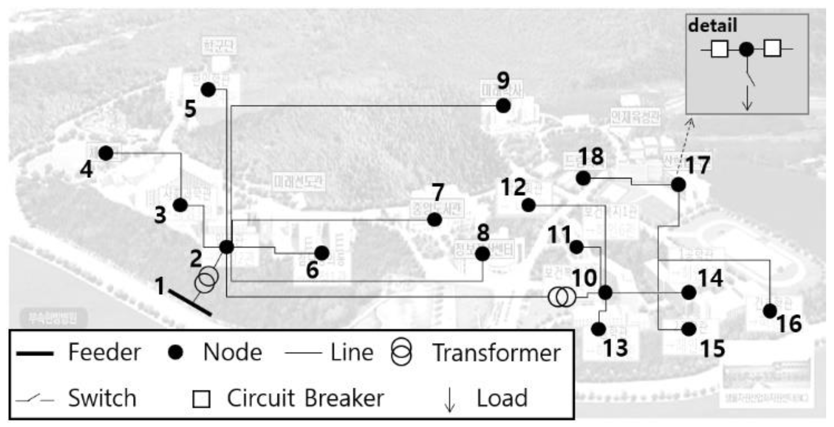
5.1.1. System Configuration

Figure 7 is the system configuration at D-university in Korea with the MGs in operation. The information regarding the peak load for each node in the system (Figure 7) is organized in

Table A1. Peak load at D-university and DG capacity for Scenarios 10, 11, 15, and 16.

Node	Peak Load [kW]	Scenario
		10	11	15	16
2	500	PV 76	PV 76 ESS 152	ESS 750
3	400	PV 62	PV 62 ESS 124	PV 50	PV 50 ESS 150
4	600	PV 243	PV 182 ESS 364	PV 100	PV 100 ESS 300
5	750	PV 96	PV 61 ESS 122
6	650	PV 86	PV 96 ESS 192	PV 100	PV 100 ESS 300
7	800	PV 20	PV 86 ESS 172
8	600		PV 20 ESS 40
9	900
10	500	PV 86 ESS 2000	PV 86 ESS 172	ESS 750
11	300
12	400			PV 50	PV 50 ESS 150
13	300
14	450	PV 58	PV 58 ESS 116
15	400	PV 50	PV 50 ESS 100	PV 50	PV 50 ESS 150
16	300			PV 50	PV 50 ESS 150
17	250	PV 223 CHP 115	PV 223 ESS 446 CHP 115	PV 100 CHP 3000	PV 100 ESS 300 CHP 3000
18	300
Total	8400	3115		5000

(Appendix A).

5.1.2. Scenarios of MG Planning (Step I)

The scenarios for MG planning, which consider the capacities of the DGs as well as their installation locations, are listed in

Table 1. Simulation condition of each Scenario for MG planning.

Scenario	DG Capacity				DG Location
	PV [kW]	ESS [kWh]	CHP [kW]	Total
1	300	400	800	1500	Node 2
2					Node 10
3					Node 18
4	800	300	400		Node 2
5					Node 10
6					Node 18
7	1000	2000	115	3115	Node 2
8					Node 10
9					Node 18
10					Ref. to Table A1
11
12	500	1500	3000	5000	Node 2
13					Node 10
14					Node 18
15					Ref. to Table A1
16

. Table A1 (Appendix A) shows the DG capacity for each node in scenarios 10, 11, 15, and 16, assuming that the DGs in Table 1 are installed at different locations.

Table 2. Ratio considering the DG types.

Scenario	ⓐ [%]	ⓑ [%]	ⓒ [%]
1–3	18	9	53
4–6		5	27
7–11	37	1	4
12–16	60	36	60

shows the ratios calculated to minutely review the distribution of the DGs. Each ratio was calculated based on the following criteria:

ⓐ:

Ratio of DG capacity to peak load

ⓑ:

Ratio of controllable DGs (CHP) to peak load

ⓒ:

Ratio of controllable DGs (CHP) to total DGs

In Table 1 and Table 2, scenarios 1–3 assume the same DG capacity but different DG installation locations (nodes 2, 10, or 18). Scenarios 4–6 have the same total DG capacity as that in scenarios 1–3 but with different ratios of the DG composition. Scenarios 7–11 have the same total DG capacity as that installed in D-university. Scenario 10 represents the actual MG in D-university, and it is the calculation result of the DG capacity to maximize the economic feasibility without consideration of resilience. To ensure resilience enhancement, the total DG capacity in scenarios 12–16 is larger than that in scenarios 7–11, and a large ratio of the CDG to peak load is assumed.

5.1.3. Simulation Condition for Estimating the Probabilistic Resilience (Step II)

To consider the various post-contingency uncertainties, the simulation conditions were examined with the following limitations [25]:

−

Type of failed facility: line, transformer, etc.

−

Fault occurrence time of each failed facility

:

Random in 0–1 h

−

Recovery time

:

Random in 4–24 h for each failed facility

5.1.4. Simulation condition for CBA (Step III)

The unit price for each cost and benefit element is presented in

Table A2. Unit price of cost and benefit elements [26].

Category		Elements		Unit Price
C	CMG	Ccapital	PV	173.8 $/kW
			CHP	1042.9 $/kW
			ESS (∼300[kWh])	608.4 $/kWh
			ESS (300[kWh]∼)	521.5 $/kWh
			EMS (H/W, S/W)	26,073.4 $
		CO&M	PV	4.3 $/kW/year
			CHP	11.3 $/kW/year
			ESS	8.7 $/kW/year
			EMS	434.6 $/year
		CDG,fuel	CHP (1[kWh] = 3.6[MJ])	0.0013 $/MJ
			ESS	0.1 $/kWh
	CUtility	CRF	CB	2607.3 $/set
			LS	1738.2 $/set
		Cbuy		0.1 $/kWh
B	BMG	BES		0.1 $/kWh
		Bsell		0.2 $/kWh
	Benviroment (1[kWh] = 0.000459 [tCO2])			19.6 $/tCO2
	BUtility	BAC		32.6 $/kW/year
		BAE		0.1 $/kWh

(Appendix A).

5.2. Simulation Result

5.2.1. Resilience Enhancement

Figure 8 shows the E-CDF result for each scenario of the three failed facilities.

Table 3. Results of EoRE.

Scenario	Number of Failed Facilities
	1	2	3	4
1	0.009	0.014	0.017	0.020
2	0.018	0.026	0.034	0.042
3	0.024	0.033	0.040	0.045
4	0.005	0.006	0.008	0.009
5	0.009	0.012	0.016	0.019
6	0.014	0.019	0.023	0.026
7	0.019	0.024	0.028	0.032
8	0.037	0.046	0.054	0.058
9	0.042	0.049	0.049	0.050
10	0.033	0.041	0.051	0.057
11	0.037	0.046	0.051	0.052
12	0.028	0.048	0.059	0.073
13	0.048	0.077	0.101	0.124
14	0.053	0.080	0.094	0.105
15	0.051	0.082	0.103	0.122
16	0.054	0.083	0.104	0.121

shows the EoRE results for one to four failed facilities. The intermediate results (resilience curve) obtained for calculating the EoRE are presented in Figure A1 (Appendix A).

In Figure 8, the E-CDF results for the scenarios with the same total capacity are similar, except for scenarios 12–16. This means that when ⓐ (the ratio of the DG capacity to peak load) in scenarios 1–11, as listed in Table 2, is small, the variation in the enhancement of resilience according to the installation locations of the DGs is negligible.

Meanwhile, although ⓐ of scenarios 7–11 is larger than ⓐ of scenarios 1–6 in Table 2, the enhancements in the resilience in scenarios 7–11 and 1–6 are similar. This is because the ratio of CDGs (ⓑ, ⓒ) in scenarios 7–11 in Table 2 is low, indicating that controllable DGs such as CHP contribute to enhancing the resilience more than the other DG types.

In Table 3, the variation in the EoRE according to changes in the number of failed facilities was significant for scenarios 12–16, which had relatively large DG capacities. Nevertheless, Scenario 12 showed a lower EoRE than scenarios 13–16 because the DGs in scenario 12 were located next to the feeder at node 2, as shown in Figure 7. These results indicate that when a failure occurs in the line connecting nodes 2 and 10 in the distribution system of Figure 7, it is more advantageous for the DGs to be installed at nodes 10 and 18 (scenarios 13 and 14) than at node 2 (scenario 12).

5.2.2. Optimal scenario based on the CBA and resilience constraint

The following resilience constraint was set to review the optimal scenario. The condition for the number of failed facilities was limited to three.

• Resilience constraint ($CR$): 0.05

Figure 9 shows the EoRE and B–C ratio for all scenarios, as well as the baseline $CR$.

Table 4. CBA result that satisfied CR.

Scenario	EoRE	Total Cost [$]	Total Benefit [$]	B–C Ratio
8	0.054	2,289,191	3,849,512	1.68
10	0.051
11	0.051	2,467,691	3,849,512	1.56
12	0.059	10,704,478	8,754,933	0.82
13	0.101
14	0.094
15	0.103
16	0.104	10,929,478	8,754,933	0.80

presents the B–C ratios for scenarios that satisfy the resilience constraint.

Table 4 shows that scenario 8, where the capacity of the NDG was relatively large, was an optimal scenario. It shows that the NDG and ESS can contribute to improving the resilience in a distribution system when the ESS capacity is more than twice the PV capacity.

However, when the reference value of the resilience constraint is set to be greater than 0.1 in Figure 9, scenario 15 (B–C ratio: 0.86) can be derived as an optimal result. This shows that the resilience (EoRE) enhancement and cost (B–C ratio) are in a trade-off relationship.

The proposed framework for MG planning can provide a cost-effective scenario by selecting scenarios that satisfy the conditions for enhancing resilience. The estimation method of probabilistic resilience included in this process provides the EoRE that considers not only the DG capacity and type but also the installation location.

6. Conclusions

This study developed a framework for MG planning considering the resilience of a distribution system as described in Section 2. In Section 3, the estimation method of the resilience curve considering the system configuration and output characteristics of the DG was presented, and the method for calculating the RI and EDF was described. In this process, the post-contingency uncertainties were considered based on the MCS. In Section 4, the CBA model was presented for various cost and benefit elements, and the EoRE was proposed to intuitively express the degree of resilience enhancement.

To consider the realistic situation of the distribution system, a case study was conducted at the D-university with an installed MG. The results in the case study showed that the proposed method for estimating the resilience could consider not only the capacity of the DGs but also their type and installation location. In addition, the proposed framework provided an optimal scenario that satisfied the resilience constraints (CR) and maximized the B–C ratio.

When the proposed framework is verified through various real systems, it could contribute to establishing a more resilient system using MG in long-term planning. Especially, the framework could be usefully utilized to establish MG of the distribution system that is oriented toward resilience enhancement, such as customers of hospitals and military and industrial facilities, because the scenarios of the MG planning that satisfy the resilience constraint are provided.

References

1. White House, Presidential Policy Directive-21—Critical Infrastructure Security and Resilience. Available online: https://obamawhitehouse.archives.gov/ (accessed on 8 February 2022).
2. North American Electric Reliability Corporation (NERC). High-Impact, Low-Frequency Event Risk to the North American Bulk Power System; 2010. Available online: https://www.energy.gov/ (accessed on 8 February 2022).
3. Panteli, M.; Mancarella, P. Influence of extreme weather and climate change on the resilience of power systems: Impacts and possible mitigation strategies. Electr. Power Syst. Res. 2015, 127, 259–270. [Google Scholar] [CrossRef]
4. Berkeley, A.R., III; Wallace, M. A Framework for Establishing Critical Infrastructure Resilience Goals; Final Report Recommendations; National Infrastructure Advisory Council: Gaithersburg, MD, USA, 2010; pp. 1–83. Available online: https://www.dhs.gov/ (accessed on 8 February 2022).
5. Wang, Y.; Huang, T.; Li, X.; Tang, J.; Wu, Z.; Mo, Y.; Xue, L.; Zhou, Y.; Niu, T.; Sun, S. A resilience assessment framework for distribution systems under typhoon disasters. IEEE Access 2021, 9, 155224–155233. [Google Scholar] [CrossRef]
6. Panteli, M.; Mancarella, P.; Trakas, D.N.; Kyriakides, E.; Hatziargyriou, N.D. Metrics and Quantification of Operational and Infrastructure Resilience in Power Systems. IEEE Trans. Power Syst. 2017, 32, 4732–4742. [Google Scholar] [CrossRef] [Green Version]
7. Cimellaro, G.P.; Reinhorn, A.M.; Bruneau, M. Framework for analytical quantification of disaster resilience. Eng. Struct. 2010, 32, 3639–3649. [Google Scholar] [CrossRef]
8. International Electrotechnical Commission (IEC). Microgrids for Disaster Preparedness and Recovery: With Electricity Continuity Plans and Systems. 2014; pp. 1–85. Available online: https://www.preventionweb.net/ (accessed on 8 February 2022).
9. Nam, Y.-H.; Lee, H.-D.; Kim, Y.-R.; Marito, F.; Kim, M.-Y.; Rho, D.-S. Economic evaluation algorithm of island micro-grid for utility and independent power producer. Trans. Korean Inst. Electr. Eng. 2017, 66, 1032–1038. [Google Scholar] [CrossRef]
10. IEEE Standards Board. 2030.9-2019—IEEE Recommended Practice for the Planning and Design of the Microgrid; IEEE: Piscataway, NJ, USA, 2019; pp. 1–45. [Google Scholar] [CrossRef]
11. Mahzarnia, M.; Moghaddam, M.P.; Baboli, P.T.; Siano, P. A Review of the Measures to Enhance Power Systems Resilience. IEEE Syst. J. 2020, 14, 4059–4070. [Google Scholar] [CrossRef]
12. Wang, Z.; Wang, J. Self-Healing Resilient Distribution Systems Based on Sectionalization into Microgrids. IEEE Trans. Power Syst. 2015, 30, 3139–3149. [Google Scholar] [CrossRef]
13. Wu, X.; Wang, Z.; Ding, T.; Wang, X.; Li, Z.; Li, F. Microgrid planning considering the resilience against contingencies. IET Gener. Transm. Distrib. 2019, 13, 3534–3535. [Google Scholar] [CrossRef]
14. Wang, Y.; Rousis, A.O.; Strbac, G. A Three-Level Planning Model for Optimal Sizing of Networked Microgrids Considering a Trade-Off Between Resilience and Cost. IEEE Trans. Power Syst. 2021, 36, 5657–5669. [Google Scholar] [CrossRef]
15. Borghei, M.; Ghassemi, M. A Multi-Objective Optimization Scheme for Resilient, Cost-Effective Planning of Microgrids. IEEE Access 2020, 8, 206325–206341. [Google Scholar] [CrossRef]
16. Weng, D. Microgrid techno-economic assessment. In Proceedings of the IRED Conference, Niagara Falls, NY, USA, 24 October 2016; Available online: https://www.osti.gov/biblio/1525094-microgrid-techno-economic-assessment-presentation (accessed on 8 February 2022).
17. Son, E.-T.; Bae, I.-S.; Kim, S.-Y.; Kim, D.-M. Facility Reinforcement Planning of Distribution System Considering Resilience. IEEE Access 2021, 9, 94272–94280. [Google Scholar] [CrossRef]
18. Che, L.; Zhang, X.; Shahidehpour, M.; AlAbdulwahab, A.; Abusorrah, A. Optimal Interconnection Planning of Community Microgrids with Renewable Energy Sources. IEEE Trans. Smart Grid 2017, 8, 1054–1063. [Google Scholar] [CrossRef]
19. Billinton, R. Evaluation of reliability worth in an electric power system. Reliab. Eng. Syst. Saf. 1994, 46, 15–23. [Google Scholar] [CrossRef]
20. Wu, X.; Shi, S.; Wang, Z. Microgrid planning considering the supply adequacy of critical loads under the uncertain formation of sub-microgrids. Sustainability 2019, 11, 4683. [Google Scholar] [CrossRef] [Green Version]
21. Son, E.-T.; Bae, I.-S.; Kim, S.-Y.; Kim, W.-W.; Kim, D.-M. A Study on the Analysis of Resilience Enhancement for the Distribution System using Microgrids. Trans. Korean Inst. Electr. Eng. P 2021, 70, 843–851. [Google Scholar] [CrossRef]
22. Shorack, G.R.; Wellner, J.A. Empirical Processes with Applications to Statistics New York; Wiley: New York, NY, USA, 1986; ISBN 0-471-86725-X. [Google Scholar]
23. Mood, A.M.; Graybill, F.A.; Boes, D.C. Introduction to the Theory of Statistics, 3rd ed.; McGraw Hill Book Company: New York, NY, USA, 1973; pp. 175–218. ISBN 100070854653. [Google Scholar]
24. Holland, P.W. Two measures of change in the gaps between the CDFs of test-score distribution. J. Educ. Behav. Stat. 2002, 27, 3–17. [Google Scholar] [CrossRef]
25. Allan, R.; Billinton, R.; Sjarief, I.; Goel, L.; So, K. A reliability test system for educational purposes-basic distribution system data and results. IEEE Trans. Power Syst. 1991, 6, 813–820. [Google Scholar] [CrossRef]
26. PG&E. Unit Cost Guide. Available online: https://www.pge.com/pge_global/common/pdfs/for-our-business-partners/interconnection-renewables/Unit-Cost-Guide.pdf (accessed on 8 February 2022).
Figure 1. MG planning framework.
Energies 15 02145 g001
Figure 2. Probabilistic estimation process of resilience based on MCS.
Energies 15 02145 g002
Figure 3. Example of resilience curve estimation.
Energies 15 02145 g003
Figure 4. Estimation process of the resilience curve.
Energies 15 02145 g004
Figure 5. Venn diagrams of nodes of time-varying topologies and sections.
Energies 15 02145 g005
Figure 6. Example of EoRE.
Energies 15 02145 g006
Figure 7. System configuration at D-university.
Energies 15 02145 g007
Figure 8. Results of E-CDF for various scenarios in failure of three facilities.
Energies 15 02145 g008
Figure 9. Results of EoRE and B–C ratio for each scenario in the failure of three facilities.
Energies 15 02145 g009