Numerical Probabilistic Load Flow Analysis in Modern Power Systems with Intermittent Energy Sources ^†

Abstract

Renewable resources integration through distributed generation (DG) affects conventional consideration of power system performance and confronts deterministic load flow (DLF) analysis with serious challenges. The DLF gives a snapshot of the system state neglecting all of the uncertainties arising from intermittent DG driven by variable weather conditions or volatile consumption. Therefore, with the aim of finer tracking and presentation of system variables, a probabilistic load flow (PLF) approach should be adopted. First, this article gives a literature overview of different PLF techniques. It focuses on numerical techniques examining them for simple random and Latin Hypercube sampling, vastly applied in previous works, and proposes a method combining Monte Carlo simulations with Halton quasi-random numbers. Stochastic modelling is performed for solar and wind power output. For method comparison and confirmation of the applicability of suggested PLF method with Halton sequences, different IEEE test cases were used, all modified by attaching DGs. More profound method assessment is conducted through discussing different renewables penetration levels and processing time. The overall simulation outcomes have shown that results of Halton method are of similar precision as the generally used Latin Hypercube method and therefore indicated the relevance of the proposed method and its potential for application in contemporary system analysis.

1. Introduction

Reliable supply of consumers with electrical energy of the prescribed quality is one of the basic goals of electrical power systems. Segmentation of vertically integrated power corporations along with the establishment of liberal electricity markets have additionally emphasized the importance of power quality and maintaining voltage parameters within the specified ranges [1].

Modern trends in the development of electrical power systems have brought an increasing demand for distributed generation (DG) based on renewable energy resources, conditioned by the requirements for slowing down climate changes through reducing greenhouse gases emitted by outdated conventional fossil fuels-based power plants. Among renewable DGs, wind farms and solar power plants have the largest share in the energy mix [2]. Their energy production capability is highly intermittent and strongly dependent on variable meteorological phenomena such as wind speed and solar irradiance, which makes them non-dispatchable units [3]. Emerging of DGs has also established a whole new category of power system elements–prosumers (i.e., consumers with the ability of generating electricity for themselves or potentially for neighboring power system).

COVID-19 crises and 2020 lock down measures in Europe have also proven the significance of renewable generation. During a period of exceptional load drop throughout the continent and lowering of nuclear and coal-based plants power output, renewable sources have taken the lead and shown their value without outstanding curtailments [4], indicating that now they are crucial and inevitable part of electrical grid.

Besides renewables, electrical vehicles (EV) have to be taken into account in analysis of the modern power systems. Their ability to be both consumers, which successfully tackle environmental requests, and storage systems, with potential to contribute to peak load shaving [5], makes EVs very useful, but also challenging in terms of their integration into power systems [6].

Bearing all previously mentioned information in mind, it is pretty clear that with every new day modern power systems have less and less in common with traditional power systems. In this regard, traditional, deterministic concept of power flow analysis (DLF), based on fixed values, can non yield an adequate accuracy of obtained results if applied on modern power systems. Simply, DLF does not take into account the uncertainties in electricity generation and consumption typical for the modern power systems with significant share of non-dispatchable units. In other words, the DLF can provide results which are valid only for a certain moment [7].

Above-mentioned novelties which gradually take greater role in electricity network demand finer tracking and presentation of systems variables. The application of a probabilistic load flow approach (PLF) could resolve this issue. Including uncertainties into calculation, the PLF application provides stochastic ranges of variables (e.g., bus voltages), which is opposed to the ranges of fixed values [8].

This article is structured as follows: Section 2 explains the main ideas, methods, and aims of load flow calculation in general. Extensive literature overview of different PLF techniques, divided into three large groups (analytical, numerical, and approximation techniques) is presented in Section 3. It focuses on Monte Carlo simulation–based numerical techniques, examining their behavior in cases of different sampling methods. First, the most basic method-simple random sampling and one of the stratified sampling methods (Latin Hypercube sampling), which were vastly applied in previous works on PLF analysis, are presented. Then a quasi-Monte Carlo PLF method combining Monte Carlo simulations with Halton quasi-random numbers is proposed with the clear intention to show its value, considering a fairly reduced number of simulation necessary for precise calculation. The theoretical background of the Halton quasi-random sequences is given in Section 4. Moreover, Section 5 provides case study simulation of the proposed methods. First, the procedure of stochastic modelling of uncertainties is shown for system variables. Actual historical meteorological records (i.e., solar and wind data) have been used and modelled by following chosen probability distribution functions (which were then sampled accordingly). For the purposes of method comparison and eventually confirmation of the applicability of the suggested PLF method, all analyses have been performed in MATLAB by using several different IEEE test cases (i.e., 14, 30 and 118 bus systems), all modified by attaching certain amount of DGs throughout the examined network. Additionally, for the sake of more profound method assessment, different penetration levels of renewable sources are considered too. Apart from results evaluation in terms of precision, they have also been discussed with regard to the processing time. Finally, our conclusions are drawn in Section 6.

This article is the extension of our research paper previously published in International Conference on Electrical, Computer, Communications and Mechatronics Engineering (ICECCME 2021) at Mauritius [9] and presented at 21st International Symposium on Power Electronics (Ee2021) at Novi Sad. Several new contributions have been added to the previous research:

• A literature review of numerical PLF analysis has been enlarged by vast number of different techniques. The article also provides substantial overview of other PLF methods, specifically analytical and approximation, establishing a systematic summary of PLF approaches which indicates their usefulness, strengths, and weaknesses;
• Furthermore, the renewable generation models of wind and solar plants have been exposed in more thorough way;
• Finally, more advanced case study simulations have been performed in terms of considered electrical system size and energy sources structure.

2. Load Flow Analyses

Load flow analysis is one of the most important and most used calculations in the field of power system analysis. The results of this calculation are crucial for the adequate planning of new and exploitation of existing parts of electrical systems. Based on the data obtained by this analysis, the needs for the construction of new system elements are considered, such as the optimal location and capacities of additional production units, transformers, power lines, reactive energy compensators, etc. It also ensures that existing elements can withstand stresses during steady-state operation. The conclusions obtained by the analysis serve to determine the optimal operation of the system with regard to economic dispatching. In addition, although the obtained data refer to the system steady-state, its algorithm is the basis for dynamic analyses of the system stability [10].

The analysis includes determination of the modules and phase angles of the bus voltages, as well as calculation of active and reactive power in the transmission (distribution) lines. The requested input data are network configuration and related parameters, power consumption and rated power and characteristics of generators.

The mathematical formulation of load flow problem is as follows [11]:

$$P_i{=U}_i{\displaystyle \sum }_{j=1}^n{U}_j{Y}_{ij}\cos \left({\theta }_i{-\theta }_j-{\vartheta }_{ij}\right)$$

(1)

$$Q_i{=U}_i{\displaystyle \sum }_{j=1}^n{U}_j{Y}_{ij}\sin \left({\theta }_i{-\theta }_j-{\vartheta }_{ij}\right)$$

(2)

where P_i and Q_i are the active and reactive power injected into node i, U_i and U_j voltage amplitudes at nodes i and j, n the total number of nodes in the system, θ_i and θ_j the phase angles of voltages at nodes i and j, and Y_ij and ϑ_ij are the amplitudes and phase angles of the corresponding nodal admittance matrix.

These formulations result in system of non-linear algebraic equations, exactly two per each node, with the exception of slack bus which has specified voltage values during the calculation. Therefore, the total number of equations is 2(n–1).

Its solution is basically achievable through some iteration processes performed by digital computers. At first, the Gauss-Seidel iterative method based on nodal admittance matrix was used. Later on, the Newton-Raphson procedure was more preferred by virtue of better convergence. One of the popular approaches is the fast P–Q decoupled method. There are also applications using the forward-backward sweep approach [12], artificial neural networks, and fuzzy algorithms [13].

In the simulation performed for the case study section of this article, the Newton-Raphson procedure was conducted. It transforms Equations (1) and (2) to a set of linear equations that connect power mismatches with voltage amplitudes and phase angles by the Jacobian system matrix:

$$\left[\begin{array}{c}\Delta P_1\\ \dots \\ \Delta P_{n-1}\\ \Delta Q_1\\ \dots \\ \Delta Q_{n-1}\end{array}\right]=\left[\begin{array}{cccccc}\frac{\partial P_1}{\partial {\theta }_1}& \cdots & \frac{\partial P_1}{\partial {\theta }_{n-1}}& \frac{\partial P_1}{\partial U_1}& \cdots & \frac{\partial P_1}{\partial U_{n-1}}\\ ⋰& \cdots & ⋰& ⋰& \cdots & ⋰\\ \frac{\partial P_{n-1}}{\partial {\theta }_1}& \cdots & \frac{\partial P_{n-1}}{\partial {\theta }_{n-1}}& \frac{\partial P_{n-1}}{\partial U_1}& \cdots & \frac{\partial P_{n-1}}{\partial U_{n-1}}\\ \frac{\partial Q_1}{\partial {\theta }_1}& \cdots & \frac{\partial Q_1}{\partial {\theta }_{n-1}}& \frac{\partial Q_1}{\partial U_1}& \cdots & \frac{\partial Q_1}{\partial U_{n-1}}\\ ⋰& \cdots & ⋰& ⋰& \cdots & ⋰\\ \frac{\partial Q_{n-1}}{\partial {\theta }_1}& \cdots & \frac{\partial Q_{n-1}}{\partial {\theta }_{n-1}}& \frac{\partial Q_{n-1}}{\partial U_1}& \cdots & \frac{\partial Q_{n-1}}{\partial U_{n-1}}\end{array}\right]\left[\begin{array}{c}\Delta {\theta }_1\\ \dots \\ \Delta {\theta }_{n-1}\\ \Delta U_1\\ \dots \\ \Delta U_{n-1}\end{array}\right]$$

(3)

System (3) can be expressed via block matrices:

$$\left[\begin{array}{c}\Delta P\\ \Delta Q\end{array}\right]=\left[\begin{array}{cc}{J}_1& J_2\\ J_3& J_4\end{array}\right]\left[\begin{array}{c}\Delta \theta \\ \Delta U\end{array}\right]$$

(4)

where J₁, J₂, J₃ and J₄ are block matrices of Jacobian whose elements are calculated as partial derivatives of Equations (1) and (2).

Newton-Raphson algorithm consists of the following steps:

• Initial values of voltage amplitudes and angles are assumed for all PQ and PV buses except for the slack bus.
• Active and reactive powers are calculated based on the assumed voltage values for all buses except the slack bus.
• Since active and reactive powers are known for PQ buses, power mismatches are calculated.
• Elements of Jacobian matrices J₁, J₂, J₃, and J₄ are calculated based on the latest available voltage and power values.
• System (3) is solved by Gaussian elimination method and voltage corrections Δθ and ΔU are obtained.
• Obtained voltage corrections are used for updating voltage values for the next iteration.
• New assumed values of voltages resulting from step 6 are used for steps 2–7. The procedure continues until power mismatch does not satisfy certain accuracy criteria.

The traditional calculation of load flow is based on a deterministic approach. This approach takes as input variables the specific values of generation and consumption (most often the average expected values), while specific values of buses voltages are provided as output variables. Based on the researchers’ experience [14], input data values for some critical regimes may be analyzed as well. The deterministic approach gives only a snapshot of the state of the system, ignoring the uncertainties arising from variable consumption or generation from renewable resources.

3. Probabilistic Load Flow

The need for a different approach in the load flow analysis and voltage quality analysis was highlighted by the European standard EN-50160 [15]. The standard promotes and requires from distribution systems certain stochastic ranges of voltages, as opposed to the ranges of fixed values.

As a possible solution, some authors have proposed the so-called stochastic calculation of load flow based on the assumption that the distributions of probabilities of the system states and the results of the load flow analysis are normally distributed. Although this assumption greatly simplifies the calculation, it has been dismissed over years as very unreliable [16].

On the other hand, a PLF analysis can take into account uncertainties regarding network configuration, consumption, weather data related to generation capability of renewable resources, equipment failure rates, etc. by the calculation based on the probability distribution of mentioned variables obtained through statistical analysis of their historical data. As a result, the states of the system (e.g., voltages) will be stochastically described too. The probabilistic approach to the calculation of load flow was first proposed in the mid-1970s [17], but has become especially popular after the growing penetration of renewable resources [18].

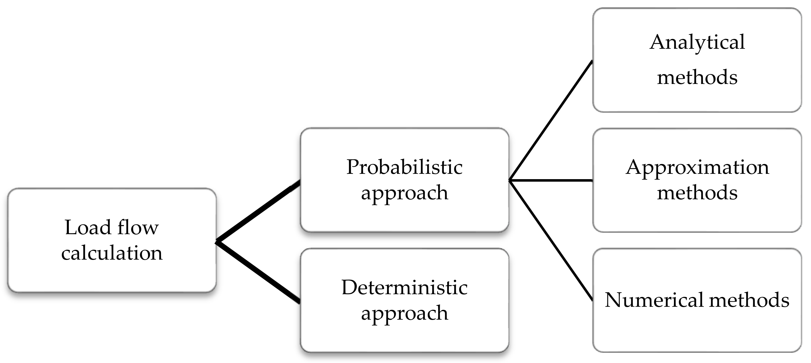
There are three groups of methods of probabilistic approach to the load flow calculation. Analytical methods, based on the convolution of probability density functions, are mathematically elegant but include a number of approximations over real systems. Numerical methods perform a large number of DLF calculations using the Monte Carlo simulation, which randomly selects input variables based on their probability density distribution functions. They are very precise but the achieving of high results accuracy is closely related to large number of iterations making these methods time-consuming. Finally, approximation methods, based on point estimation technique, mitigate the computational burden of numerical methods by statistical approximations.

Figure 1 presents the classification of different approaches to the load flow calculation.

3.1. Analytical Methods

The main concept of analytical approach is strictly mathematical, performing the convolution of known probability density distribution functions of produced and consumed power and obtaining the probability density distribution functions of the corresponding stochastic variable system states [19]. Nevertheless, the load flow equations are nonlinear and the input variables in various buses of electrical grid are often dependent. Therefore, the application of convolution of probability functions demands some approximations such as linearization of load flow equations; assumptions about complete independence or at least linear dependence between input variables; modelling of generation and load with Gaussian distribution; and consideration of the grid configuration and parameters as constant.

Load flow equations linearization by developing them in the Taylor series is primarily performed for certain expected values of input variables [20]. The results precision is evidently becoming deteriorated for values that are far from the corresponding average values. These errors are mostly notable at the ends of the voltage distribution curve, which can lead to misleading conclusions about the voltage quality and eventually bad decisions affecting system development process.

With the aim of mitigating the effects of linearization, several methods have been proposed, particularly those involving multilinearization [21], i.e., equation linearization around several values (instead of only one), with convolution being performed for each of them in order to obtain the probability distributions of the results, which are eventually combined into a single result. This approach yields more reliable results than simple linearization. Additional accuracy is achieved by applying the method presented in [22] which combines multilinearization and Monte Carlo method by conducting multilinearization based on the total active load of the system and then performing DLF for the considered points.

When it comes to the efficiency of the convolution process, the initial procedures were based on the application of the Laplace transformation [23]. Improving efficiency, in terms of processing time required, can be achieved by applying a fast Fourier transformation [24], although the calculation is still very extensive.

Another analytical approach to power flow calculation considers the analysis of input variables that are discretely distributed or not represented by a Gaussian distribution by approximating them by the weighted sum of the components modelled by the Gaussian distribution [25]. However, this method is neither faster than the application of Fourier transformation nor more precise than multilinearization techniques.

An interesting idea is the application of sequence operation theory proposed in [26]. Input variables are represented as probability sequences which are processed using standard sequence operations. The results indicate the efficiency of the method in case of discrete input variables, while the main drawback is the inability to establish variable interdependency.

One big subgroup of analytical methods consists of techniques based on cumulants combined with series expansion. Their major advantage is the reduction of calculation time in comparison to classical convolution methods due to the usage of algebraic operations rather than convolution procedures [27]. Gram–Charlier expansion is widely used [28,29], but it works with unimodal distributions only [27]. On the other hand, Cornish–Fisher expansion performs better with non-Gaussian distributions [30]. Nevertheless, its usage might cause precision problems in side regions of the obtained probability distribution [31].

It should be noted that problems with cumulant methods occur when working with dependent random variables. Improvement in [32] proposes modelling of dependent variables as functions of several independent variables by using Cholesky decomposition.

An additional problem with cumulants can be the error caused by great fluctuations of input variables (e.g., wind speed) [33]. This article suggests generating samples of random variables by inverse Nataf transformation and grouping these samples into clusters by k-means algorithm. This leads to mitigation of sample variance inside a cluster. The procedure continues with cumulant operations.

Besides combining cumulants with series expansion, there are proposals of combing them with maximum entropy algorithm [34], Laplace transformation [35] or multiple integrals [36].

3.2. Approximation Methods

Approximation methods calculate general statistical features describing considered stochastic variables. The most of them is based on point estimation technique which was first proposed in [37]. Their key advantage over classical Monte Carlo simulation-based numerical methods is the computational simplicity despite the fact they also use DLF calculation. Moreover, for using point estimation it is enough to know the basic characteristics of random variable, such as mean value, variance, skewness and kurtosis coefficients. Aim of the method is to calculate moments of distribution of output variables as functions of initially known moments of input variables. At the end it is necessary to apply one of the series expansion techniques, e.g., Gram–Charlier or Cornish–Fisher.

There have been many improvements to the basic method. In [38] it was extended for the application for non-symmetrical random variables, while in [39] the precision was enhanced in case of small number of input variables. In [40] the method was used to analyse an unbalanced three-phase system. The use of asymmetric point estimation for systems with wind turbines and photovoltaic panels is presented in [41]. Improving accuracy can be achieved by covering a larger number of points. However, this requires the calculation of higher-order moments which can be very challenging. In contrast, in [42] the accuracy was improved by adding a new pair of points with the first three known moments.

Some other approximation methods are the application of unscented transformation which is useful due to the ease of working with dependent random variables and nonlinear equations [43] as well as the usage of Taguchi’s orthogonal arrays requiring fewer DLF calculations when applied to balanced systems with renewables [44] or to three-phase systems with dependencies between variables [45].

3.3. Numerical Methods

Numerical methods of PLF calculation are based on applying Monte Carlo simulation–the procedure consisting of stochastic simulations using random variables. Taking the calculated probability density functions of input variables as a base, values of generated power coming from renewable power plants and the consumption values are randomly selected and then the DLF calculation is performed for them. The simulation must be repeated for a certain number of times so that the obtained values (e.g., node voltages) can be statistically processed and presented in form of their probability density functions.

The key advantage of numerical methods is their precision which originates from the ability to apply nonlinear equations for load flows analysis, in contrast to analytical methods when these equations have to be transformed into a computationally simpler form. Due to the accuracy, these methods are used for comparison with all other probabilistic methods and for assessing their adequacy. Nevertheless, applying the Monte Carlo method and completing the required number of iterations can take a significant amount of time. With the development of computer technology, this shortcoming is slowly being alleviated but still remains very problematic.

As for the number of iterations that need to be performed when using this method, that number does not depend on the size of the analyzed system. It can be a fixed number assumed on the basis of experience or be related to a certain coefficient of variation which determines the convergence of the method.

Monte Carlo simulation-based methods can be grouped based on sampling technique [46]. The most basic one is simple random sampling. Its main drawback is the possibility of sampling a value that is very similar to the values from previous iterations. This is the reason of extremely big number of iterations needed to cover the analyzed set of data correctly. In order to improve the efficiency of calculations, quasi-random sampling methods based on low discrepancy sequences have been introduced. One of them is the Latin Hypercube technique which samples one value from the interval and then removes that whole interval from further analysis. However, the usage of this sampling technique generates undesired dependencies between sampled values. This is solved by various permutation methods (e.g., Cholesky decomposition) [47]. In [48] Latin Hypercube sampling is combined with copula method which allows predefining the dependencies between random variables. Additionally, Ref. [49] analyses the application of correlation matrices which are not positively definite by combining Nataf transformation, Latin Hypercube sampling and matrices decomposition to singular values. One of the quasi-Monte Carlo methods, the Latin Supercube, which is in fact a combination of digital nets and the Latin Hypercube method is presented in [50] showing the results of satisfactory accuracy compared to similar numerical methods.

Moreover, Uniform Design sampling technique was used in [51]. First, random numbers following uniform distribution between 0 and 1 are generated by this technique. Then, the marginal transformation is used for transforming the generated numbers to values of desired distribution of input random variables. Finally, values are permuted based on rank correlations in order to reflect correlations between them.

In [52], improved Sobol generator of quasi-random numbers assuring the efficiency in one hand and Johnson system giving the precision of modelled probability distribution in the other hand were utilized.

Improvement of the efficiency of Monte Carlo method is also analyzed through the application of non-parametric density estimations of load flow calculation results. Their advantage is the flexibility of modelling a given dataset which cannot give analytical solution or the solution would be too complicated. One of the estimation methods is the adaptive kernel density estimation based on smoothing features of linear diffusion demonstrated in [53], which gave the results faster than classical Monte Carlo method. In [54], the application of Parzen Window density estimation was suggested indicating the simplicity of approach in situations with limited input data.

An overview of developed different PLF methods which have been discussed above is presented in

Table 1. Overview of developed PLF methods.

Analytical methods	Linearization using Taylor series Multilinearization Laplace transformation Fast Fourier transformation Cumulant methods: - Gram–Charlier expansion - Cornish–Fisher expansion - Cholesky decomposition - Inverse Nataf transformation and k-means clustering - Maximum entropy algorithm - Laplace transformation - Multiple integrals Sequence operation theory Approximation of variables by the weighted sum of the Gauss-modelled components
Approximation methods	Point estimation technique Asymmetric point estimation Unscented transformation Taguchi’s orthogonal arrays
Numerical methods	Simple random sampling Latin Hypercube: - Cholesky decomposition - Copula method - Nataf transformation Latin Supercube Uniform Design sampling Sobol quasi-random numbers Adaptive kernel density estimation Parzen Window density estimation

.

3.4. Research Gap

Having considered above-listed set of approaches to PLF analysis, it can be observed that in cases of numerical techniques usage, the biggest challenge is the balance between accuracy and number of analyzed samples. As opposed to simple random sampling, low discrepancy sequences sampling has usually been performed. One of the most used and described methods is Latin Hypercube sampling.

On the other hand, the viability of application of Halton quasi-random sequences, which provide better uniformity over the Latin Hypercube technique, has been diminished and very slightly analyzed.

Halton sequences are usually implemented for the evaluation of integrals. They are considered to be easy to calculate but have issues with regards to output stability [55].

The central point of this article is to examine their feasibility for PLF problem solving by comparing them to the commonly used numerical methods–namely, simple random sampling–as the reference method and Latin Hypercube sampling–as widely utilized method in similar research works.

4. Halton Sequences

Halton sequence is one of the classical statistical sequences used for generating points for Monte Carlo simulation. It was first described in [56]. Despite being deterministic, by virtue of its low-discrepancy it can be considered random for various applications. This sequence generalizes van der Corput sequence and is very easy to implement [57] since it is based on the radical inverse function:

$${\varphi }_p\left(n\right)\equiv \frac{b_0}{p}+\frac{b_1}{p}+\dots +\frac{b_m}{p^{m+1}}$$

(5)

where p is a prime number, and the p-ary expansion of n is given as n = b₀ + b₁p + … + b_mp^m, with integers 0 ≤ b_j < p.

The Halton sequence, X_n, in s-dimensions is then defined as:

$$X_n=({\varphi }_{p_1}\left(n\right),{\varphi }_{p_2}\left(n\right),\dots ,{\varphi }_{p_s}\left(n\right))$$

(6)

where the dimensional bases p₁, p₂, …, p_s are pairwise coprime. In practice, always the first s primes are used as the bases.

One of the main disadvantages of the Halton sequence is that its quality becomes easily degraded in case of large dimensional problems. The root of this problem comes from the correlations between the radical inverse functions for different dimensions [58]. One option to overcome the issue is to leap over the specific number of points and omit them for each point taken. It is important that the number of point leaped over is different from all bases.

Additionally, in order to avoid correlations among different dimensions and other undesirable properties related to initial points of a sequence, first 1000 values were skipped in all simulations presented in this article.

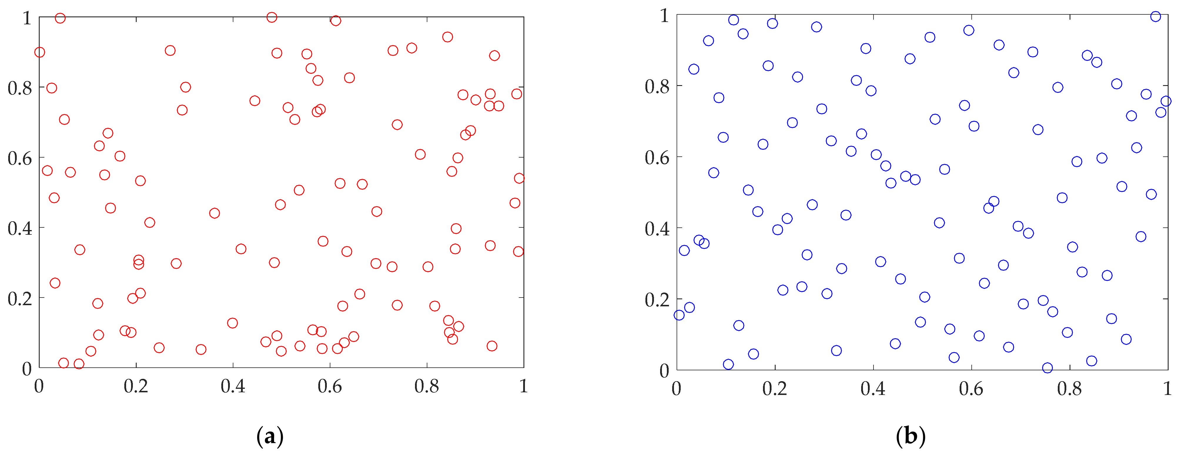
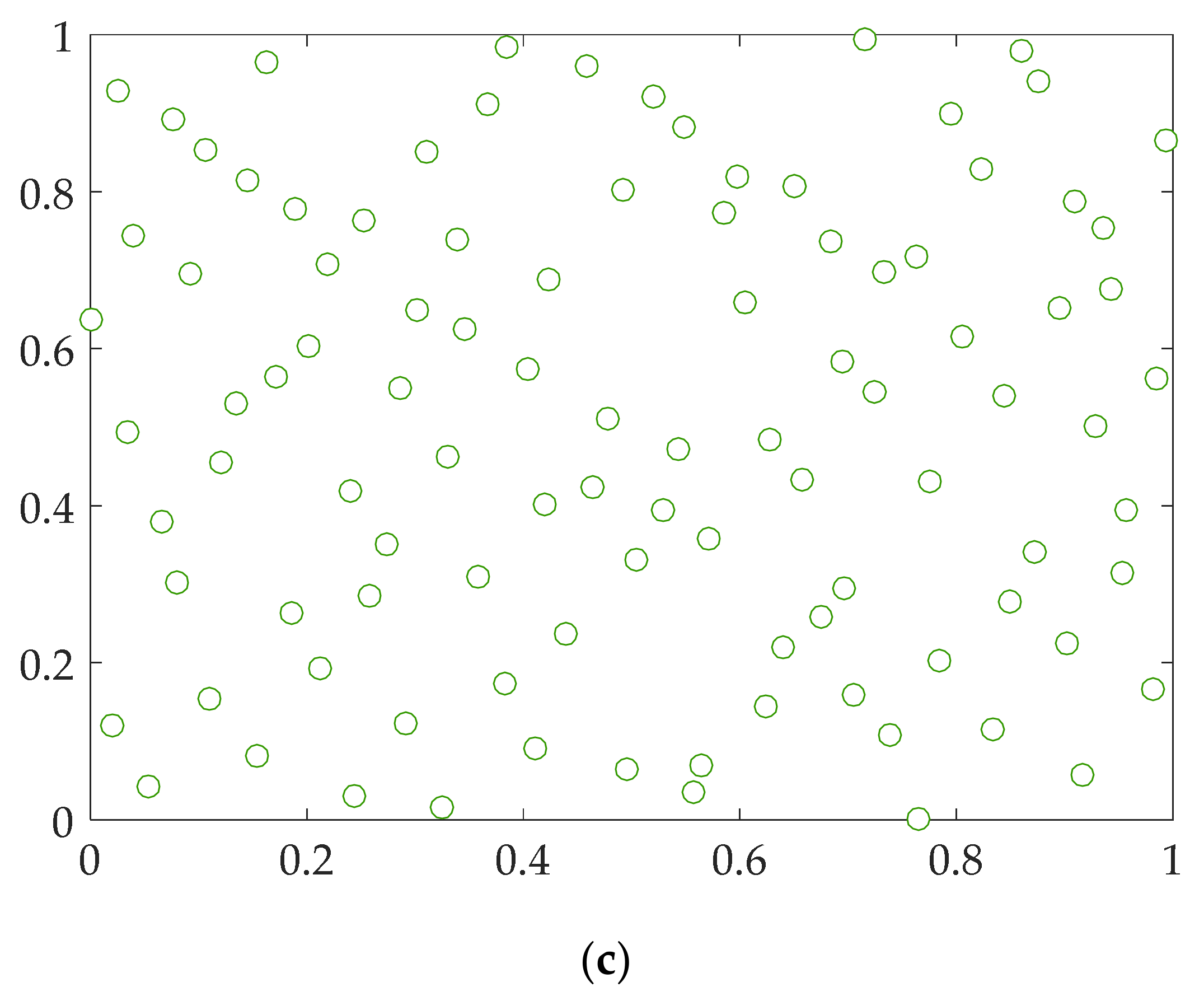
As an illustration of sampling characteristics and quality, Figure 2 demonstrates sampling 100 two-dimensional points chosen by simple random, Latin Hypercube and Halton sampling respectively.

5. Case Study

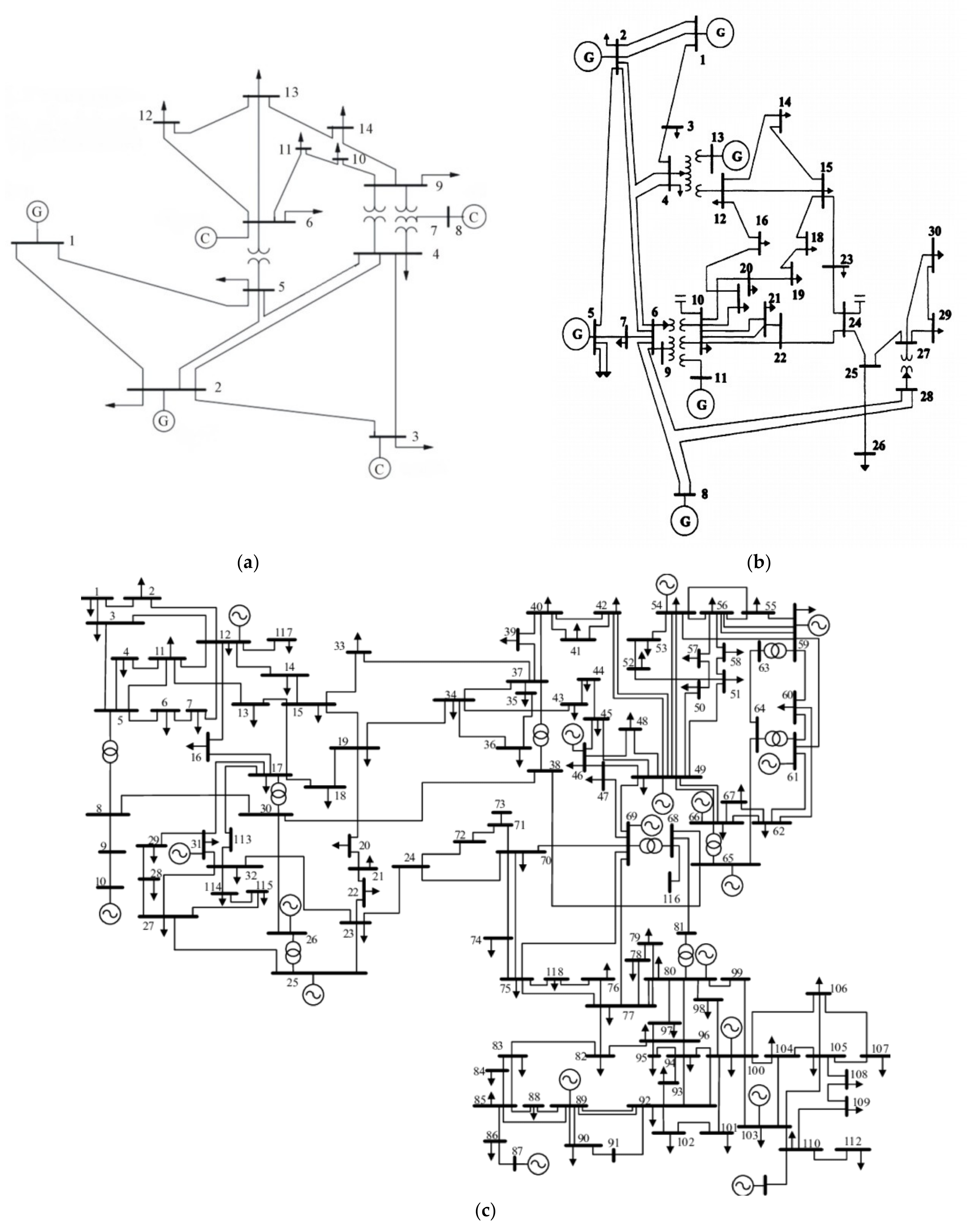
For the purpose of simulation of numerical PLF methods used with different sampling techniques, as well as for the comparison of the obtained results, IEEE test systems of 14, 30, and 118 nodes were considered [59].

All three systems were modified by attaching additional wind and solar generators to specific bus loads. They were modelled as negative load quantities and attached to specific bus loads as follows:

$$P_i{=P}_{i, load}-P_{DG}$$

(7)

$$Q_i{=Q}_{i, load}-Q_{DG}$$

(8)

where P_{i, load} and Q_{i, load} are initial active and reactive power values at bus i as specified by the chosen test system configuration, P_DG and Q_DG active and reactive power of DGs attached to bus i and P_i and Q_i total active and reactive power values at bus i. The reactive power of DGs is calculated based on assumed power factor cos(φ) = 0.95.

Renewable sources penetration levels of 30% and 60% of total consumption load were examined.

No specific advanced generator model has been implemented for conventional generators. They have been fully approximated and treated as PV buses.

Figure 3 shows the configuration of the IEEE 14 [60], 30 [61], and 118 [62] bus test systems.

5.1. Modeling Uncertainties

5.1.1. Load Model

The load was stochastically modelled by the normal distribution [63], taking the deterministic value of the load as the mean value and 5 per cent of the assumed mean value as the value of the standard deviation. Therefore, the probability density function of the load can be expressed as:

$$f\left(x\right)=\frac{1}{\sigma \sqrt{2\mathsf{\pi }}}·e^{\frac{-{\left(x-\mu \right)}^2}{{2\sigma }^2}}$$

(9)

where x is the bus load, µ the mean value, and σ the standard deviation of load.

5.1.2. Wind Speed and Generator Model

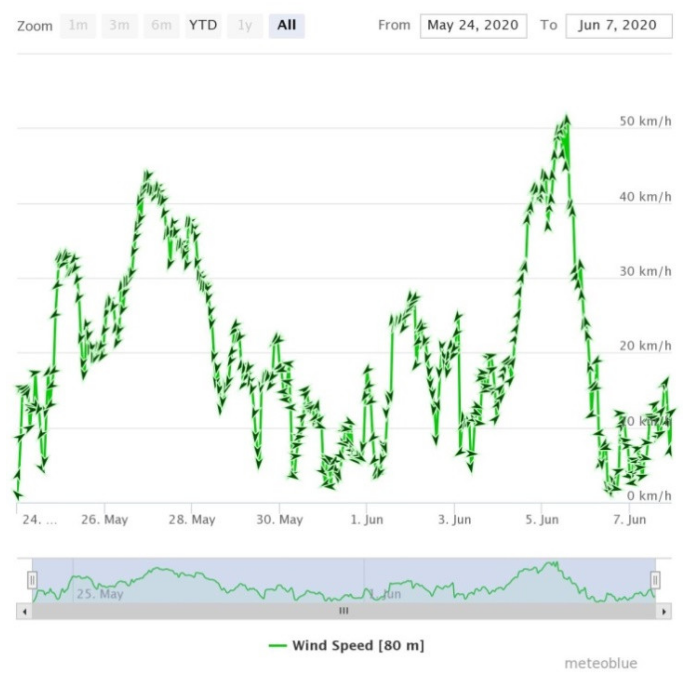
For purposes of this simulation, real wind speed data were used. They had been taken from the online historical weather reports [64], for the period from 24 May to 7 June 2020, for the site Krnovo (meteorologically interesting area in Montenegro, altitude-1500 m), at the height of 80 metres above the ground. Figure 4 shows a graph of wind speed during the above-mentioned time period.

Firstly, the histogram representing wind speed was created using the Distribution Fitting Tool in the MATLAB software package (MATLAB R2016a, The MathWorks, Inc., Natick, MA, USA). Secondly, the wind speed was stochastically modelled by the Weibull distribution [65] and the parameters of scale and shape of the probability distribution density function were obtained.

The histogram with the modelled wind density probability distribution function obtained through the MATLAB distribution fitting tool is given in Figure 5.

Rated power of wind turbine is chosen considering voltage level and size of the used IEEE test systems. Based on the chosen rated power, an average onshore wind turbine is selected for the simulation. Its characteristics are shown in

Table 2. Wind turbine characteristics.

Parameters	Values
Rated power	2.8 MW
Rated speed	12 m/s
Cut-in speed	2.5 m/s
Cut-out speed	25 m/s
Blade length	50 m
Power coefficient	0.4
Power factor	0.95

.

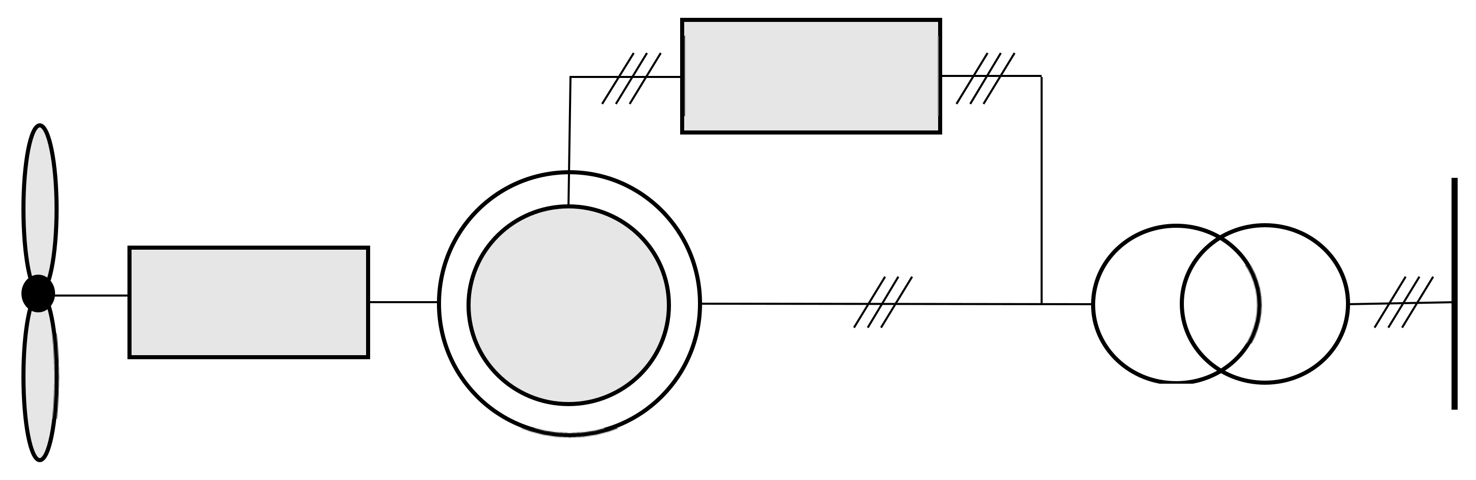
The generation model used in this article has been based on doubly fed induction generator which is vastly used for wind turbines. Its scheme is presented in Figure 6. The main idea of this model is that stator windings are directly connected to the electrical network while rotor winding are connected via back-to-back voltage source convertor. It enables the generator to remain synchronized with the grid while its speed (i.e., frequency) can differ from the grid frequency. It also offers control of rotor speed by the variation of frequencies of currents that feed the rotor, which is important for maintaining power system stability.

The output power of wind generator P is determined by the Equation (10):

$$\mathrm{P}\left(v\right)=\left\{\begin{array}{c}{0, v<v}_{in}\\ \frac{1}{2}·C_p·N_b·N_g·\rho ·A·v^3{, v}_{in}{<v<v}_r\\ P_r{, v}_r{<v<v}_{out}\\ {0, v}_{out}<v\end{array}\right.$$

(10)

where v is wind speed, v_in cut-in speed, v_out cut-out speed, v_r rated wind speed, P_r rated wind generator power, C_p power coefficient, N_b generator efficiency, N_g gearbox/bearings efficiency, ρ air density, and A surface affected by wind. The dependence of output power of wind generator on wind speed calculated based on above mentioned characteristics is shown in Figure 7.

For purposes of this simulation, the power output of a wind farm is considered to be the sum of power outputs of multiple wind generators constituting the farm.

5.1.3. Solar Generation Model

For purposes of modelling solar generator power output based on real data, online tool NREL’s PWVatts [66] has been used. Hourly values of irradiance and temperature covering one year for the area of central Montenegro were taken into consideration for calculating the power output which is defined by formula:

$$P_{PVout}=\eta ·L·\frac{I_{\mathrm{tr}}}{1000}·P_{\mathrm{dc}0}·\left(1+\gamma ·\left(T-25 °\mathrm{C}\right)\right)$$

(11)

where η is inverter efficiency, L system losses, I_tr POA irradiance, P_dc0 DC System Size, γ temperature coefficient and T photovoltaic cell temperature [67]. Characteristics of the solar generator are shown in

Table 3. Solar generator characteristics.

Parameters	Values
DC System Size	4 MW
Cell Material	Crystalline Silicon
Approximate Nominal Efficiency	15%
Temperature Coefficient of Power	−0.47%/°C
System Losses	14.08%
DC to AC Size Ratio	1.2
Inverter Efficiency	96%
Ground Coverage Ratio	0.4

.

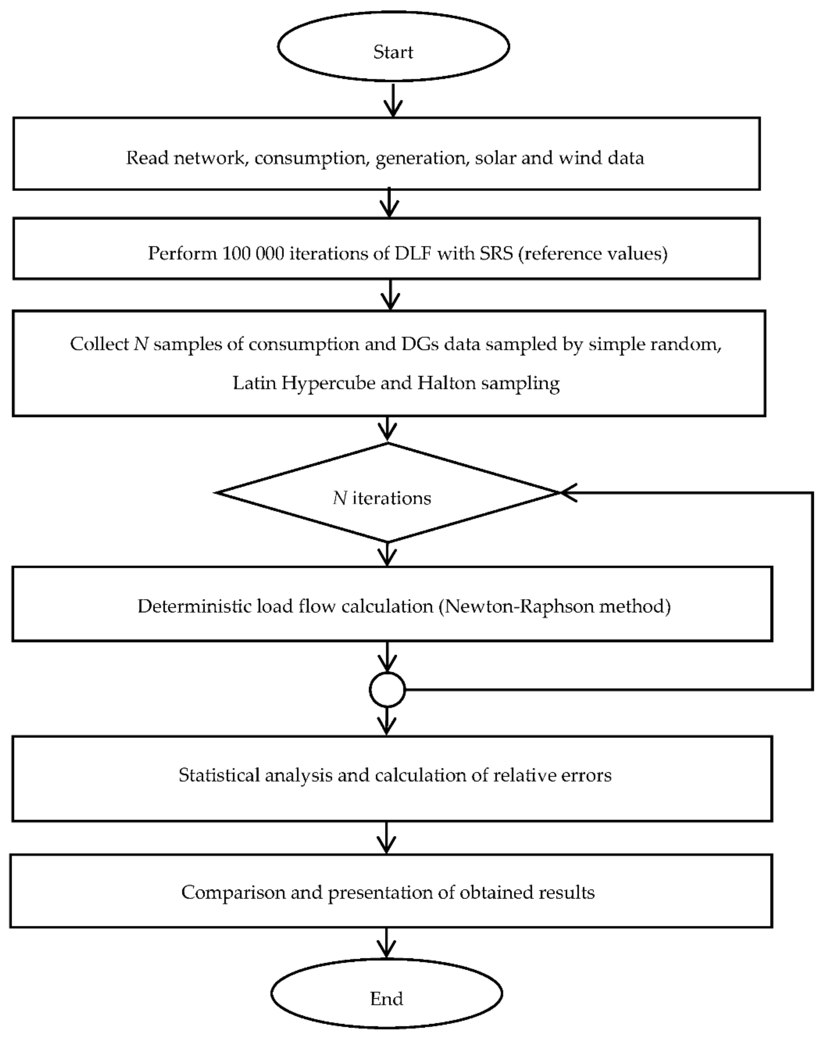
5.2. Simulation Algorythm

First, 100,000 values of consumption, wind and solar generation data are sampled by simple random sampling and used for the same number of DLF calculations by applying MATPOWER, a package of MATLAB M-files prepared for solving power flow and optimal power flow simulation problems [68].

Having in mind that the focal point of this article is probabilistic performance of power flow calculation, the simplest form of analyses has been utilized. One bus in each test system has been declared as slack bus used for handling all power imbalances but also as reference bus for voltage angle values. By default, nonlinear Equations (1) and (2) are iteratively solved by standard Newton-Raphson method in polar form using a full Jacobian which is updated in every iteration. At each iteration step, the method performs calculating the power mismatch for known PQ nodes, forming the Jacobian based on the sensitivities of these mismatches to changes of computed voltage values and solving for an updated set of these value by factorizing the Jacobian.

It is important to mention that the implemented power flow solver ignores any limits and constraints related to generators, branch flows, voltage quantities, etc. with intention to avoid broadening the analyses. Additionally, no frequency regulation has been dealt with in this research.

The results obtained in all iterations are stored and eventually statistically modelled by the normal probability distribution based on the calculated mean values and values of the standard deviation. They are considered as reference values for further simulations.

Then, a specified number of stochastic variable values N is sampled three times by different sampling techniques: simple random, Latin Hypercube, and Halton quasi-random sampling methods. All of these datasets are then used for DLF calculation in separate iterations. The results are compared with reference values and the relative error is calculated as follows:

$${\mathsf{\epsilon }}_{r, N}\left(x\right)=\left|\frac{x^N{-x}_{ref}}{x_{ref}}\right|·100\%$$

(12)

where x_ref is reference value calculated after 100,000 iterations and x^N is output value obtained after N iterations.

It is important to notice that the Latin Hypercube and Halton methods, as quasi-random, always give the same result for the specific number of iterations, while simple random sampling is completely random method (i.e., gives different values).

Several simulation scenarios with datasets consisting of 50, 100, 500, and 1000 values were considered in order to assess the accuracy and calculation time and eventually to examine methods’ applicability in real life system analysis.

On the other hand, the same simulation is performed for two different levels of integrated renewable generation (30% and 60% of total consumption load).

Figure 8 shows the algorithm of the applied program.

The simulations were performed on HP Pavilion device with Intel Core i-5, 2.5 GHz processor and 8 GB RAM, using the MATLAB software package, version 2016a.

5.3. Simulation Scenarios

Several simulation scenarios were considered in order to assess the impact of system size as well as the DG level presence to load flow calculation. Consequently IEEE 14, 30, and 118 bus test systems were chosen to be compared in terms of system size. On the other hand, effects of DG were modelled by attaching sets of wind and solar generators to some nodes of the grid. Review of all simulation scenarios is given in

Table 4. Review of simulation scenarios.

IEEE Test System Size	DG Penetration Level	Sampling Method
14 buses	30% 60%	Simple random sampling
30 buses		Latin Hypercube sampling
118 buses		Halton sequences

.

5.4. Results

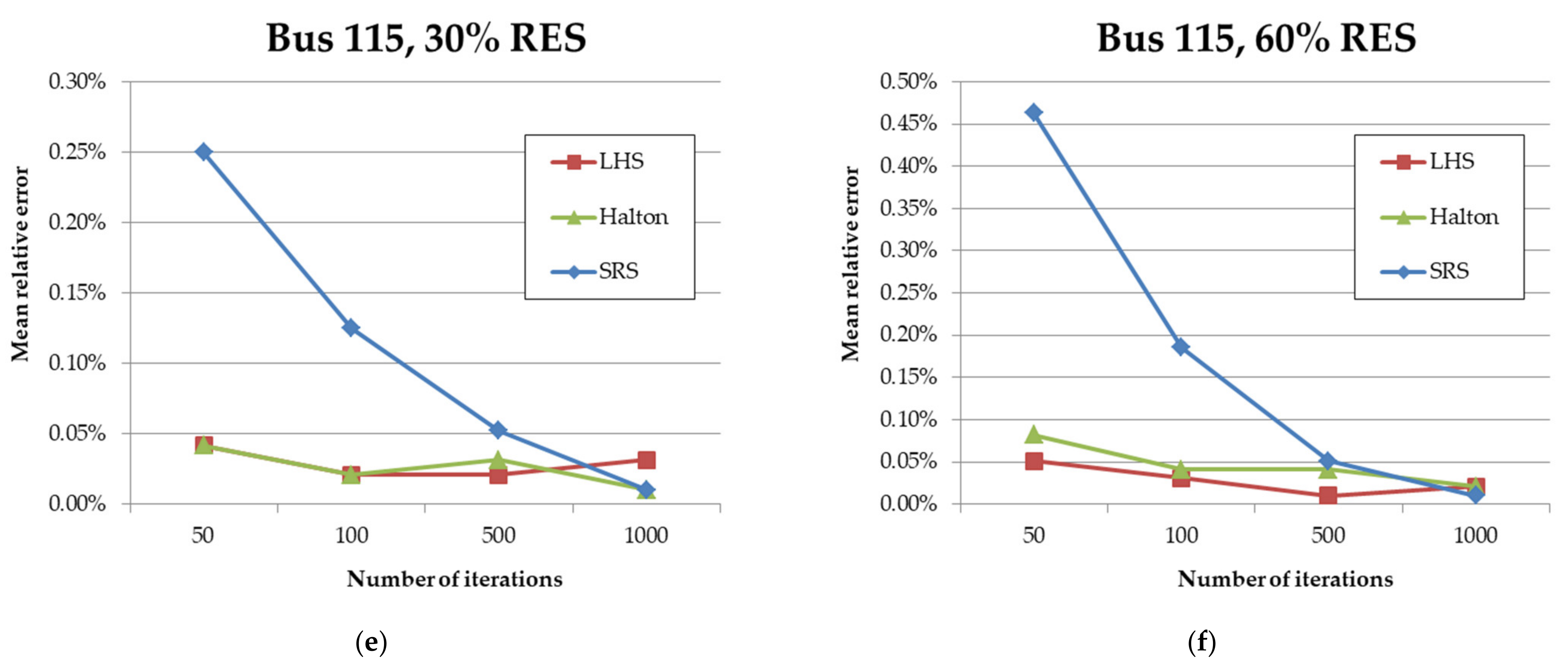
To compare the results of the application of PLF calculation performed with input values obtained by different sampling methods, several subtypes of simulations have been performed for four above mentioned datasets/iteration sizes (50, 100, 500, 1,000) varying system size and DG penetration level. Figure 9 shows mean relative errors of voltages at node 14 of IEEE 14 bus system, node 8 of IEEE 30 bus system and node 115 of IEEE 118 bus test system, respectively, obtained after three subtype simulations–SRS, LHS and Halton, for all proposed numbers of iterations and DG penetrations.

After adding wind and solar generators to certain buses of the analyzed test system, a problem in terms of voltage increase is expected in nearby nodes, with exception to the buses connected to conventional generators and compensators.

Based on the simulation results, we can observe the values of relative errors of voltages obtained by calculation performed with simple random sampling, Latin Hypercube, or Halton quasi-random sampling, and it is clear that the latter two approaches give a more realistic picture of the state of the system after the reasonably small number of iterations.

For example, let’s consider the voltage value at bus 14 of IEEE 14 bus system. At first the relative error of calculated voltage is approximately seven times bigger after applying SRS sampling in contrast to two quasi-random methods which almost immediately give accurate results. Similar conclusion can be drawn if we consider relative error of voltage at bus 115 of IEEE 118 bus system. The ratio of above-mentioned results is 25:1 in case of 30% and 47:1 in case of 60% of added renewable resources. The simulations indicate that Halton-based sampling is comparable to the efficiency of Latin Hypercube and can be applied equally as numerical PLF approach to power systems with lots of renewable resources.

Furthermore, as to the variation of DG penetration level, we can see that the error of simple random sampling method rises as more renewable generators are added to the electrical network. On the other hand, the Latin Hypercube and Halton methods keep precision despite the increase of uncertainty in the system.

Moreover, it is important to mention that the error of quasi-random sampling becomes higher for bigger power systems. For example, in IEEE 14 bus system it is around 1%, in IEEE 30 bus system 3% and in IEEE 118 bus test system up to 8%. However, this error is minor in contrast to the one occurring in case of simple random sampling.

It is also evident that Halton sampling is more accurate than Latin Hypercube for smaller systems (e.g., 14 and 30 bus test systems) which indicates its issue with high dimensional problems. Nevertheless, the difference between the two methods in case of 118 bus system is hardly worth mentioning. This overall suggests equal importance and the applicability of the proposed Halton sampling-based PLF.

Additionally,

Table 5. Calculation time for different simulation scenarios.

Iteration	Simple Random	Latin Hypercube	Halton
50	2.55	3.07	3.01
100	2.91	3.36	3.43
500	4.71	5.31	5.26
1000	6.72	7.77	7.67
100,000	592.19	-	-

presents the average calculation time in seconds required for execution of analyzed simulation scenarios.

It is clear that the simulation time is pretty much similar for the same number of iterations. Nevertheless, Latin Hypercube and Halton methods offer acceptable results after three seconds, while simple random sampling provides the results of tolerable accuracy only after 1000 of iterations which take at least twice as much time.

6. Conclusions

In this article, numerical method for probabilistic load flow calculation based on Halton quasi-random sequences was proposed and compared to basic simple random sampling and widely used Latin Hypercube sampling techniques. The focus of the research was the contemporary power system containing various uncertainties arising from the renewable resources generation and high variation of consumption due to introduction of prosumers. At first, an extensive literature review providing wide division of different probabilistic load flow methods was given. Mathematical background to Halton sequences was presented too.

Numerous types of simulations, which varied system sizes, sampling techniques and DG penetration levels, have been performed. The initial idea was that simple random sampling-based PLF is totally unusable in terms of accuracy, when applied for quick probabilistic analysis performed by small number of iterations. It was suggested that Halton sampling could tackle this issue in a similar manner as Latin Hypercube method.

The results confirmed the expectations since the calculated relative errors of bus voltages have proven to be significantly less in case of applying Halton sampling, supporting the claim of its superiority over basic simple random sampling approach, as well as the effectiveness of its usage for the load flow analysis, voltage quality assessment, and planning of modern power system.

Furthermore, performed simulations imply that the dominance of Halton sampling could be even more noticeable as the renewable generators penetration in the power system rises. This point positions Halton sampling PLF calculation as one of the methods that we will count on gradually more in future.

It should be noted that a more realistic model of production and consumption values could be obtained by analyzing their interdependence, both in terms of meteorological conditions and by taking into account seasonal trends. Also, further improvement could be the modelling of wind speed by second resolution, when the values of wind speed are not independent in time but depend on the previous ones.

In addition, further research on this topic should be performed on real test systems which could give more genuine review taking into account practical limitations.

Nevertheless, considering current rising penetration of DGs, the forthcoming mass integration of electric vehicles into the power system and also the very dynamic development of energy storage systems, a probabilistic approach to load flow analysis supported by quasi–Monte Carlo techniques can be expected to become an indispensable tool in power system development.

References

- Sencar, M.; Pozeb, V.; Krope, T. Development of EU (European Union) energy market agenda and security of supply. Energy 2014, 77, 117–124. [Google Scholar] [CrossRef]
- REN21 Secretariat. Renewables 2020—Global Status Report; REN21 Secretariat: Paris, France, 2020. [Google Scholar]
- Perera, A.T.D.; Nik, V.M.; Mauree, D.; Scartezzini, J.L. Electrical hubs: An effective way to integrate non-dispatchable renewable energy sources with minimum impact to the grid. Appl. Energy 2017, 190, 232–248. [Google Scholar] [CrossRef]
- Werth, A.; Gravino, P.; Prevedello, G. Impact analysis of COVID-19 responses on energy grid dynamics in Europe. Appl. Energy 2021, 281, 116045. [Google Scholar] [CrossRef] [PubMed]
- Solanke, T.U.; Ramachandaramurthy, V.K.; Yong, J.Y.; Pasupuleti, J.; Kasinathan, P.; Rajagopalan, A. A review of strategic charging–discharging control of grid-connected electric vehicles. J. Energy Storage 2020, 28, 101193. [Google Scholar] [CrossRef]
- Wu, C.; Wen, F.; Lou, Y.; Xin, F. Probabilistic load flow analysis of photovoltaic generation system with plug-in electric vehicles. Int. J. Electr. Power Energy Syst. 2015, 64, 1221–1228. [Google Scholar] [CrossRef]
- Conti, S.; Raiti, S. Probabilistic load flow for distribution networks with photovoltaic generators part 1: Theoretical concepts and models. In Proceedings of the International Conference on Clean Electrical Power, Capri, Italy, 21–23 May 2007; pp. 132–136. [Google Scholar]
- Zakaria, A.; Ismail, F.B.; Lipu, M.S.H.; Hannan, M.A. Uncertainty models for stochastic optimization in renewable energy applications. Renew. Energy 2020, 145, 1543–1571. [Google Scholar] [CrossRef]
- Mišurović, F.; Mujović, S. Probabilistic load flow analysis using Halton sequences in power systems with renewable resources. In Proceedings of the International Conference on Electrical, Computer, Communications and Mechatronics Engineering (ICECCME), Mauritius, Mauritius, 7–8 October 2021; pp. 1–6. [Google Scholar]
- Wang, X.-F.; Song, Y.; Irving, M. Load flow analysis. In Modern Power Systems Analysis; Springer: Boston, MA, USA, 2008; pp. 71–128. [Google Scholar]
- Anastasiadis, A.G.; Voreadi, E.; Hatziargyriou, N.D. Probabilistic load flow methods with high integration of renewable energy sources and electric vehicles—Case study of Greece. In Proceedings of the IEEE Trondheim PowerTech Conference, Trondheim, Norway, 19–23 June 2011; pp. 1–8. [Google Scholar]
- Jabari, F.; Shamizadeh, M.; Mohammadi-Ivatloo, B. Probabilistic power flow analysis of distribution systems using Monte Carlo simulations. In Optimization of Power System Problems—Studies in Systems, Decision and Control; Pesaran, M.P., Mohammadi-Ivatloo, B., Eds.; Springer: Cham, Switzerland, 2020; p. 262. [Google Scholar]
- Buragohain, U.; Boruah, T. Fuzzy logic based load flow analysis. In Proceedings of the International Conference on Algorithms, Methodology, Models and Applications in Emerging Technologies (ICAMMAET), Chennai, India, 16–18 February 2017; pp. 1–6. [Google Scholar]
- Sexauer, J.M.; Mohagheghi, S. Voltage Quality Assessment in a Distribution System With Distributed Generation—A Probabilistic Load Flow Approach. IEEE Trans. Power Deliv. 2013, 28, 1652–1662. [Google Scholar] [CrossRef]
- EN 50160:2010; Voltage Characteristics of Electricity Supplied by Public Distribution Systems. European Committee for Electrotechnical Standardization (CENELEC): Brussels, Belgium, 2010.
- Chen, P.; Chen, Z.; Bak-Jensen, B. Probabilistic load flow: A review. In Proceedings of the Third International Conference on Electric Utility Deregulation and Restructuring and Power Technologies, Nanjing, China, 6–9 April 2008; pp. 1586–1591. [Google Scholar]
- Borkowska, B. Probabilistic Load Flow. IEEE Trans. Power Appar. Syst. 1974, PAS-93, 752–759. [Google Scholar] [CrossRef]
- Prusty, B.R.; Jena, D. A critical review on probabilistic load flow studies in uncertainty constrained power systems with photovoltaic generation and a new approach. Renew. Sustain. Energy Rev. 2017, 69, 1286–1302. [Google Scholar] [CrossRef]
- Allan, N.; Borkowska, B.; Grigg, H. Probabilistic analysis of power flows. Proc. Inst. Electr. Eng. 1974, 121, 1551–1556. [Google Scholar] [CrossRef]
- Allan, N.; Al-Shakarchi, M.R.G. Probabilistic a.c. load flow. Proc. Inst. Electr. Eng. 1976, 123, 531–536. [Google Scholar] [CrossRef]
- Allan, N.; Leite da Silva, A.M. Probabilistic load flow using multilinearisations. IEE Proc. C Gener. Transm. Distrib. 1981, 128, 280–287. [Google Scholar] [CrossRef]
- Leite de Silva, A.M.; Arienti, V.L. Probabilistic load flow by a multilinear simulation algorithm. IEE Proc. C Gener. Transm. Distrib. 1990, 137, 276–282. [Google Scholar] [CrossRef]
- Allan, N.; Grigg, H.; Al-Shakarchi, M.R.G. Numerical techniques in probabilistic load flow problems. Int. J. Numer. Methods Eng. 1976, 10, 853–860. [Google Scholar] [CrossRef]
- Allan, N.; Leite da Silva, A.M.; Abu-Nasser, A.A.; Burchett, C. Discrete Convolution in Power System Reliability. IEEE Trans. Reliab. 1981, R-30, 452–456. [Google Scholar] [CrossRef]
- Sirisena, H.R.; Brown, E.P.M. Representation of non-Gaussian probability distributions in stochastic load-flow studies by the method of Gaussian sum approximations. IEE Proc. C Gener. Transm. Distrib. 1983, 130, 165–171. [Google Scholar] [CrossRef]
- Prusty, B.R.; Jena, D. Sequence operation theory based probabilistic load flow assessment with photovoltaic generation. In Proceedings of the Michael Faraday IET International Summit, Kolkata, India, 12–13 September 2015; pp. 164–169. [Google Scholar]
- Sanabria, L.A.; Dillon, T.S. Stochastic power flow using cumulants and Von Mises functions. Int. J. Electr. Power Energy Syst. 1986, 8, 47–60. [Google Scholar] [CrossRef]
- Usaola, J. Probabilistic load flow in systems with wind generation. IET Gener. Transm. Distrib. 2009, 3, 1031–1041. [Google Scholar] [CrossRef]
- Yuan, Y.; Zhou, J.; Ju, P.; Feuchtwang, J. Probabilistic load flow computation of a power system containing wind farms using the method of combined cumulants and Gram–Charlier expansion. IET Renew. Power Gener. 2011, 5, 448–454. [Google Scholar] [CrossRef]
- Usaola, J. Probabilistic load flow with wind production uncertainty using cumulants and Cornish–Fisher expansion. Int. J. Electr. Power Energy Syst. 2009, 31, 474–481. [Google Scholar] [CrossRef]
- Fan, M.; Vittal, V.; Heydt, G.T.; Ayyanar, R. Probabilistic Power Flow Studies for Transmission Systems with Photovoltaic Generation Using Cumulants. IEEE Trans. Power Syst. 2012, 27, 2251–2261. [Google Scholar] [CrossRef]
- Cai, D.; Chen, J.; Shi, D.; Duan, X.; Li, H.; Yao, M. Enhancements to the Cumulant Method for probabilistic load flow studies. In Proceedings of the IEEE Power and Energy Society General Meeting, San Diego, CA, USA, 22–26 July 2012; pp. 1–8. [Google Scholar]
- Deng, X.; Zhang, P.; Jin, K.; He, J.; Wang, X.; Wang, Y. Probabilistic load flow method considering large-scale wind power integration. J. Mod. Power Syst. Clean Energy 2019, 7, 813–825. [Google Scholar] [CrossRef]
- Williams, T.; Crawford, C. Probabilistic Load Flow Modeling Comparing Maximum Entropy and Gram-Charlier Probability Density Function Reconstructions. IEEE Trans. Power Syst. 2013, 28, 272–280. [Google Scholar] [CrossRef]
- Kenari, M.; Sepasian, M.; Setayesh Nazar, M.; Mohammadpour, H.A. Combined cumulants and Laplace transform method for probabilistic load flow analysis. IET Gener. Transm. Distrib. 2017, 11, 3548–3556. [Google Scholar] [CrossRef]
- Wu, W.; Wang, K.; Li, G.; Jiang, X.; Wang, Z. Probabilistic load flow calculation using cumulants and multiple integrals. IET Gener. Transm. Distrib. 2016, 10, 1703–1709. [Google Scholar] [CrossRef]
- Rosenblueth, E. Point estimates for probability moments. Proc. Natl. Acad. Sci. USA 1975, 72, 3812–3814. [Google Scholar] [CrossRef]
- Rosenblueth, E. Two-point estimates in probabilities. Appl. Math. Model. 1981, 5, 329–333. [Google Scholar] [CrossRef]
- Caro, E.; Morales, J.M.; Conejo, A.J.; Minguez, R. Calculation of Measurement Correlations Using Point Estimate. IEEE Trans. Power Deliv. 2010, 25, 2095–2103. [Google Scholar] [CrossRef]
- Caramia, P.; Carpinelli, G.; Varilonec, P. Point estimate schemes for probabilistic three-phase load flow. Electr. Power Syst. Res. 2010, 80, 168–175. [Google Scholar] [CrossRef]
- Soroudi, A.; Aien, M.; Ehsan, M. A Probabilistic Modeling of Photo Voltaic Modules and Wind Power Generation Impact on Distribution Networks. IEEE Syst. J. 2012, 6, 254–259. [Google Scholar] [CrossRef]
- Che, Y.; Wang, X.; Lv, X.; Hu, Y. Probabilistic load flow using improved three point estimate method. Int. J. Electr. Power Energy Syst. 2020, 117, 105618. [Google Scholar] [CrossRef]
- Aien, M.; Fotuhi-Firuzabad, M.; Aminifar, F. Probabilistic Load Flow in Correlated Uncertain Environment Using Unscented Transformation. IEEE Trans. Power Syst. 2012, 27, 2233–2241. [Google Scholar] [CrossRef]
- Hong, Y.; Lin, F.; Yu, T. Taguchi method-based probabilistic load flow studies considering uncertain renewables and loads. IET Renew. Power Gener. 2016, 10, 221–227. [Google Scholar] [CrossRef]
- Carpinelli, G.; Rizzo, R.; Caramia, P.; Varilone, P. Taguchi’s method for probabilistic three-phase power flow of unbalanced distribution systems with correlated Wind and Photovoltaic Generation Systems. Renew. Energy 2018, 117, 227–241. [Google Scholar] [CrossRef]
- Ramadhani, U.H.; Shepero, M.; Munkhammar, J.; Widén, J.; Etherden, N. Review of probabilistic load flow approaches for power distribution systems with photovoltaic generation and electric vehicle charging. Int. J. Electr. Power Energy Syst. 2020, 120, 106003. [Google Scholar] [CrossRef]
- Yu, H.; Chung, Y.; Wong, K.P.; Lee, H.W.; Zhang, J.H. Probabilistic Load Flow Evaluation with Hybrid Latin Hypercube Sampling and Cholesky Decomposition. IEEE Trans. Power Syst. 2009, 24, 661–667. [Google Scholar] [CrossRef]
- Cai, D.; Shi, D.; Chen, J. Probabilistic load flow computation using Copula and Latin hypercube sampling. IET Gener. Transm. Distrib. 2014, 8, 1539–1549. [Google Scholar] [CrossRef]
- Zhang, J.; Xiong, G.; Meng, K.; Yu, P.; Yao, G.; Dong, Z. An improved probabilistic load flow simulation method considering correlated stochastic variables. Int. J. Electr. Power Energy Syst. 2019, 111, 260–268. [Google Scholar] [CrossRef]
- Hajian, M.; Rosehart, W.D.; Zareipour, H. Probabilistic Power Flow by Monte Carlo Simulation with Latin Supercube Sampling. IEEE Trans. Power Syst. 2013, 28, 1550–1559. [Google Scholar] [CrossRef]
- Cai, D.; Shi, D.; Chen, J. Probabilistic load flow with correlated input random variables using uniform design sampling. Int. J. Electr. Power Energy Syst. 2014, 63, 105–112. [Google Scholar] [CrossRef]
- Zhang, L.; Cheng, H.; Zhang, S.; Zeng, P.; Yao, L. Probabilistic power flow calculation using the Johnson system and Sobol’s quasi-random numbers. IET Gener. Transm. Distrib. 2016, 10, 3050–3059. [Google Scholar] [CrossRef]
- Soleimanpour, N.; Mohammadi, M. Probabilistic Load Flow by Using Nonparametric Density Estimators. IEEE Trans. Power Syst. 2013, 28, 3747–3755. [Google Scholar] [CrossRef]
- Rouhani, M.; Mohammadi, M.; Kargarian, A. Parzen Window Density Estimator-Based Probabilistic Power Flow with Correlated Uncertainties. IEEE Trans. Sustain. Energy 2016, 7, 1170–1181. [Google Scholar] [CrossRef]
- Mohammed, N. Comparing Halton and Sobol Sequences in Integral Evaluation. Zanco J. Pure Appl. Sci. 2019, 31, 32–39. [Google Scholar]
- Halton, J.H. On the efficiency of certain quasi-random sequences of points in evaluating multi-dimensional integrals. Numer. Math. 1960, 2, 84–90. [Google Scholar] [CrossRef]
- Weerasinghe, G.; Chi, H.; Cao, Y. Particle Swarm Optimization Simulation via Optimal Halton Sequences. Procedia Comput. Sci. 2016, 80, 772–781. [Google Scholar] [CrossRef]
- Kocis, L.; Whiten, W.J. Computational investigations of low-discrepancy sequences. ACM Trans. Math. Softw. 1997, 23, 266–294. [Google Scholar] [CrossRef]
- Power Systems Test Case Archive, University of Washington. Available online: http://labs.ece.uw.edu/pstca (accessed on 1 June 2021).
- Ahmad, F. Enhancement of the Voltage Profile for an IEEE-14 Bus System by Using FACTS Devices. In Applications of Computing, Automation and Wireless Systems in Electrical Engineering; Lecture Notes in Electrical Engineering; Mishra, S., Sood, Y., Tomar, A., Eds.; Springer: Singapore, 2019; p. 553. [Google Scholar]
- De, M.; Goswami, S.K. A Direct and Simplified Approach to Power-flow Tracing and Loss Allocation Using Graph Theory. Electr. Power Compon. Syst. 2010, 38, 241–259. [Google Scholar] [CrossRef]
- Fernandez-Porras, P.; Panteli, M.; Quiros-Tortos, J. Intentional Controlled Islanding: When to Island for Power System Blackout Prevention. IET Gener. Transm. Distrib. 2018, 12, 3542–3549. [Google Scholar] [CrossRef]
- Billinton, R.; Huang, D. Effects of Load Forecast Uncertainty on Bulk Electric System Reliability Evaluation. IEEE Trans. Power Syst. 2008, 23, 418–425. [Google Scholar] [CrossRef]
- Meteoblue. Available online: http://www.meteoblue.com (accessed on 10 June 2020).
- Constante-Flores, G.E.; Illindala, M. Data-driven probabilistic power flow analysis for a distribution system with Renewable Energy sources using Monte Carlo Simulation. In Proceedings of the IEEE/IAS 53rd Industrial and Commercial Power Systems Technical Conference (I&CPS), Niagara Falls, ON, CA, 6–11 May 2017; pp. 1–8. [Google Scholar]
- PVWatts® Calculator. The National Renewable Energy Laboratory (NREL). Available online: https://pvwatts.nrel.gov/index.php (accessed on 10 May 2021).
- Dobos, A.P. PVWatts Version 5 Manual; Techical Report; The National Renewable Energy Laboratory (NREL): Golden, CO, USA, 2014.
- Zimmerman, D.; Murillo-Sanchez, E.; Thomas, J. Matpower: Steady-State Operations, Planning and Analysis Tools for Power Systems Research and Education. IEEE Trans. Power Syst. 2011, 26, 12–19. [Google Scholar] [CrossRef]