Machine Learning Algorithms for Flow Pattern Classification in Pulsating Heat Pipes

Abstract

Owing to their simple construction, cost effectiveness, and high thermal efficiency, pulsating heat pipes (PHPs) are growing in popularity as cooling devices for electronic equipment. While PHPs can be very resilient as passive cooling systems, their operation relies on the establishment and persistence of slug/plug flow as the dominant flow regime. It is, therefore, paramount to predict the flow regime accurately as a function of various operating parameters and design geometry. Flow pattern maps that capture flow regimes as a function of nondimensional numbers (e.g., Froude, Weber, and Bond numbers) have been proposed in the literature. However, the prediction of flow patterns based on deterministic models is a challenging task that relies on the ability of explaining the very complex underlying phenomena or the ability to measure parameters, such as the bubble acceleration, which are very difficult to know beforehand. In contrast, machine learning algorithms require limited a priori knowledge of the system and offer an alternative approach for classifying flow regimes. In this work, experimental data collected for two working fluids (ethanol and FC-72) in a PHP at different gravity and power input levels, were used to train three different classification algorithms (namely K-nearest neighbors, random forest, and multilayer perceptron). The data were previously labeled via visual classification using the experimental results. A comparison of the resulting classification accuracy was carried out via confusion matrices and calculation of accuracy scores. The algorithm presenting the highest classification performance was selected for the development of a flow pattern map, which accurately indicated the flow pattern transition boundaries between slug/plug and annular flows. Results indicate that, once experimental data are available, the proposed machine learning approach could help in reducing the uncertainty in the classification of flow patterns and improve the predictions of the flow regimes.

1. Introduction

The lifespan and reliability of a wide range of electronic components and electro-mechanical assemblies are often compromised by the poor performance of the thermal control system (TCS). Cooling capacity, weight, and cost requirements are becoming very challenging in high-density PCBs, microprocessors, photovoltaic solar arrays, and actuators, not only limiting the expected performance [1] but also creating safety issues, as in EV battery systems [2]. On the other hand, energy consumption for cooling purposes has critically increased in recent years. Data centers consume 200 TWh each year worldwide [3], where 38% (76 TWh) is estimated to go toward cooling processes. There are a wide variety of available cooling processes for electronics. The most common methods based on two-phase flow are flow boiling [4,5,6,7,8,9,10], pool boiling [11,12,13,14], and impinging jets [15,16,17,18].

Pulsating heat pipes (PHPs) can play a leading role in reducing cooling costs due to their resulting equivalent thermal conductivity that is several times higher than that of pure copper [19]. Furthermore, no pumping power is required for the circulation of the working fluid. This results in a sensible reduction in complexity, volume, and weight of the TCS. The PHP is a thermally driven heat transfer device patented in the 1990s [20,21], which has seen a growing research interest since then. It is simpler in its construction and more cost-effective, compared to other similar heat transfer devices (e.g., heat pipes, loop heat pipes). It is composed either of a tube bent in several turns or of two plates welded with a serpentine-like path milled on one of the surfaces. Once filled and sealed, a working fluid resides in the PHP as an alternation of liquid slugs and vapor plugs due to the dominant effect of capillary forces with respect to buoyancy. When heat is applied to the evaporator zone, the fluid motion inside the tube is activated, and the pressure fluctuations drive a self-excited [22] oscillating motion of liquid plugs and vapor bubbles, also identified as oscillating Taylor flow. This condition significantly enhances the heat transfer [23] by exploiting both sensible and latent heat.

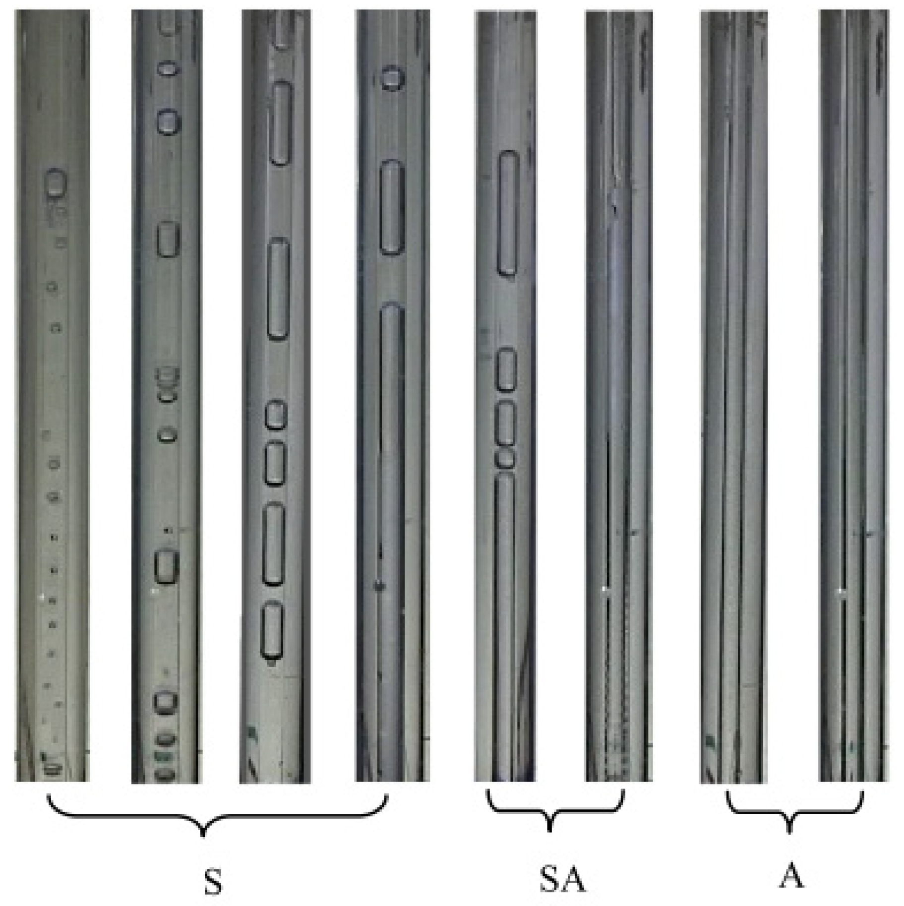
1.1. Flow Patterns in PHPs

Whilst PHPs are drawing the attention of a growing number of research groups, including both experimental and numerical approaches, the industrialization of such technology is still in its preliminary phase, and examples of off-the-shelf PHPs are not yet common and limited to specific applications. The complex interplay of evaporation/condensation phenomena, surface tension, and inertial effects has been the object of several numerical investigations with the aim of developing a robust modeling tool. Nikolayev [24] developed one of the first models able to describe the chaotic self-sustained oscillations in a PHP with an arbitrary number of branches and arbitrary number of bubbles. Further improvements of the same model led to the implementation of the effect of the tube conductivity on the start-up phase [25] and the impact of the PHP orientation on the overall performance [26].

The operation of a PHP is strongly linked to the existence of a dominant slug/plug flow throughout the required range of operating conditions. Due to the variation of flow direction, pressure drop, and liquid film thickness in a PHP, several flow patterns have been observed [27], showing transitions between slug/plug, semi-annular, and annular flow (Figure 1). For a given geometry, the flow pattern is highly influenced by filling ratio and power input [28], due to the effect on the vapor quality, showing a higher ratio of bubble length over tube diameter [29]. As a result, the slug/plug flow pattern can transition into an annular flow, which in the long run can lead to a reduction in thermal performance and a stoppage of the oscillation due to critical drying out of the evaporator. The flow pattern has been extensively investigated in flow boiling in millimeter-scale channels, and it is the result of the interaction of interfacial, inertial, viscous, and gravitational forces. Without an exhaustive knowledge of the flow pattern, the correct thermal and hydraulic design parameters cannot be calculated properly. Despite the crucial role played, the majority of the available flow boiling pressure drop correlations have been formulated without reference to the flow pattern condition they covered [30]. It is also known that the available heat transfer correlations are very sensitive to the flow pattern condition [31]. Frequently, the expected flow pattern is roughly linked to the dimension of the channel. A rough classification proposed by Kandlikar [32] fixed 3 mm as the transition limit between macro-channels and micro-channels, not considering fluid properties, inertial effects, and gravity levels. In varying gravity conditions, a transition from a thermosyphon mode (semi-annular dominant) to PHP mode (slug/plug dominant) impacts the thermal performance, operating range, and start-up power [33].

One of the main limitations of the available numerical tools is the inability to define the dominant flow pattern given a set of operating conditions. The flow pattern is assumed a priori, and only static criteria are considered. Bond number ($Bo=\rho g{d}^2/\sigma$), or its relevant form considering the wettability through the contact angle $(\theta <90°)$ $(Bo=\rho g{d}^2/\left(\sigma cos\theta )\right)$, and the confinement number ($Co=1/B{o}^{1/2}$) are implemented to establish whether the initial existence condition for slug/plug flow are met. Once the motion is activated, there is no real control of the transitions of the flow pattern, mainly ignoring inertial effects. Break-ups and coalescence events were reviewed in a numerical investigation from Andredaki et al. [34]. An approach to the development of flow pattern maps for oscillating flows based on dimensionless numbers was proposed by Pietrasanta et al. [29], drawing the attention to break-up and coalescence phenomena in a simplified PHP loop, suggesting the effective use of the actual bubble acceleration rather than the static, nominal g value (i.e., gravitational acceleration) and the actual bubble velocity to describe the transition between slug/plug and semi-annular flow. This last methodology, even if much more accurate than the use of Bond number and other dimensionless numbers such as Weber or Reynolds number, has the disadvantage that it cannot be used for design purposes, but only for a posteriori validation of numerical codes.

Therefore, despite the great effort shown so far, the development of comprehensive design tools, validated over a wide range of operating conditions and able to assist thermal engineers, is not yet complete.

1.2. Machine Learning Algorithms for Two-Phase Flow Heat Transfer

Machine learning is a rapidly growing field that allows data-driven optimization, and it has been recently extended to flow identification and design of cooling devices at different scales, considering the most significant design parameters as inputs and flow regimes or thermal resistance as outputs, depending on the application. The use of these algorithms is predominant in regression problems for heat transfer coefficients and pressure drop, although the classification of flow patterns can still be found in the available literature.

Several challenges related to two-phase flow heat transfer have been addressed via the use of machine learning techniques. The prediction of flow patterns using support vector machines (SVMs) was proposed by Guillén-Rondon et al. [35]. Here, the authors trained an SVM with a large two-phase flow pattern dataset and achieved on average 95% prediction accuracy when testing the algorithm on different groups and combinations of flow patterns. Another interesting contribution is within flow boiling and condensation heat transfer. The prediction of heat transfer coefficients for both phase changes is a challenging task, and the use of machine learning has proven to be beneficial for facilitating these estimations. An example is the work by Zhu et al. [36] which proposed the use artificial neural networks (ANNs) to predict flow boiling and condensation heat transfer coefficients for micro-channel systems with serrated fins. The authors were able to identify the most relevant geometrical and operational parameters to minimize the prediction error and evaluate the influence of specific operational parameters such as mass and heat flux into the prediction accuracy of the ANN. The results were promising, showing that the relative deviation from experimental data was on average 11.4% and 6.10% for flow boiling and condensation, respectively. The use of ANN is also useful in image recognition and analysis. A recent study published by Suh et al. [37] established an automated framework for determining boiling curves from high-quality bubble images using convolutional neural networks (CNNs). The image analysis performed by the neural network was able to capture relevant physical features used for its training and learning of the underlying statistics between bubble dynamics and corresponding boiling curves. The prediction error was reported to be 6% on average.

In terms of the identification of flow patterns in PHP systems, few attempts were found. Most efforts focused on common heat pipes and two-phase systems. Hernandez et al. [38] developed a decision-tree-based classifier to identify flow regimes and select appropriate predictive models for several two-phase flow systems. Zhang et al. [39] proposed two different machine learning classification algorithms for two-phase nuclear systems. The first one was designed for real-time flow regime identification based on SVMs, and the second classifier was designed for transient flow regime classification using CNNs. Both classifiers performed with high accuracy, allowing for a fast response when dealing with complex two-phase systems. Note that the above-mentioned contributions are related to two-phase flow systems, where no pulsating phenomenon occurs, and the transition from one flow regime to another may be less rapid than when the flowrate and its direction are not controlled (as it is the case with PHP systems).

In the context of PHP devices, most research attempts have dedicated their efforts to the prediction of key design parameters, such as thermal resistance and pressure drop. Jokar et al. [40] presented a novel approach for simulation and optimization of PHPs, based on a multilayer perceptron (MLP) neural network. According to the authors, PHPs, as a complex system, can be successfully simulated by means of artificial neural networks. Jalilian et al. [41] extended the study to the optimization of a flat plate PHP for application in a solar collector. The trained network was validated with experimental data and used to evaluate the objective function to maximize the thermal efficiency of the system. A comprehensive discussion of the thermal performance prediction of PHPs based on an artificial neural network (ANN) and regression/correlation analysis (RCA) was proposed by Patel and Metha [42]. The authors investigated the influence of nine major input variables, considering more than 1600 experimental points from the literature. Wang et al. [43] proposed a similar predicting model based on ANN for the optimization of the effects of different working fluids, extending the current state-of-the-art approaches.

Table 1. Relevant studies on machine learning applied to PHPs.

Author	Year	Model Description	Input Parameters	Output	Prediction Accuracy
Jokar et al. [40]	2016	Combination of ANN and GA 2 hidden layers (50 and 40 neurons) Batch learning method 70% of data used for training	Heat flux Inclination angle Filling ratio	Equivalent thermal resistance	Relative errors of 5–12%
Jalilian et al. [41]	2016	ANN to describe behaviour of PHP in solar collectors GA for optimizing design parameters of solar collector	Solar radiation PHP evaporator length Filling ratio Water tank temperature Inclination angle	Heat gained by collector	Root-mean-square error between 7% and 13%
Patel and Mehta [42]	2018	ANN as a prediction model RCA to find correlation among input and outputs Data collected from 2003 to 2017	Geometrical parameters Working fluids Operational parameters	Thermal resistance	Correlation coefficient of 0.89 for ANN and 0.95 for RCA with dimensionless numbers
Wang et al. [43]	2019	General model for varied working fluids and conditions Use of ANN for prediction Evaporation and condensation temperature estimated from model	Dimensionless numbers related to heat transfer and system geometry Ratio of evaporation length and diameter	Thermal resistance	Mean square error of 0.014 and correlation coefficient of 0.98

summarizes the main input parameters and machine learning approaches adopted in the abovementioned work. Note that the implementation of these machine learning algorithms is rather recent, indicating that there are still further studies to perform, although promising results have been obtained.

On the basis of the findings shown in Table 1, there is still a need for understanding the complex phenomenon of flow regime transition in PHP systems, and for the classification of the flow pattern when the device is in operation. The capability of identifying the flow regime for a set of operating conditions allows for a more accurate prediction of design parameters and for useful insights regarding the behavior of the system during operation. Within this context, the use of machine learning is beneficial, as it leverages the abundance of significant sets of data. The advantages of machine learning techniques, namely, the direct use of data, the variety of methods for specific purposes, and their equation-free nature, provide unique characteristics that can improve the optimization of experiment design, speed in experimental analysis, and scaling to different scenarios.

This work proposes, for the first time, the use of machine learning classifiers to identify flow patterns and flow pattern transition in a single-loop PHP system with two different working fluids and in varying gravity conditions using data from the European Space Agency Parabolic Flight Campaigns [11,25]. Since the single-loop PHP allows the visualization of flow patterns, this makes the present analysis unique in understanding if ML can be successfully trained to recognize PHP flow patterns. The selection of the most suitable classifier is carried out by comparing the accuracies of such classifiers when predicting the flow regime on unseen data (or testing sets). The selected classifier is used for devising flow pattern maps for both working fluids, to identify the location of the flow regime transition zone. It is expected that this capability provides a more systematic approach when identifying flow regimes, reducing observation uncertainty (when used).

2. Methodology

This work was carried out in two stages. First, the experiments were performed, where the data used for the machine learning implementation were generated. Second, these data were preprocessed and prepared for the deployment of machine learning tests and analysis. Velocity measurements were used to estimate acceleration, as described in the work done by Pietrasanta et al. [44]. The length of bubbles was also measured. Pressure measurements also took place in both thermal terminals of the device (i.e., condenser and evaporator). These measurements were used to estimate physical properties for the calculation of dimensionless numbers such as Reynolds (Re), Weber (We), Froude (Fr), and Bond (Bo) numbers, as defined in Pietrasanta et al. [29]. The labeling process was conducted visually while analyzing the high-speed images. These values, along with the label for each observation, were used to train the machine learning algorithms. Note that the entire set of data was split into a training and testing subsets. Cross-validation within the training set was also implemented for hyperparameter selection.

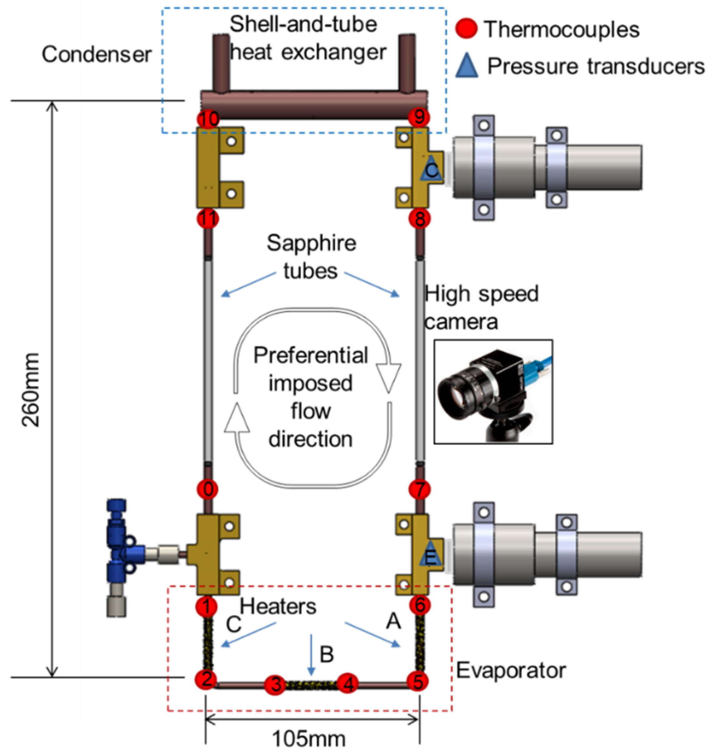
2.1. Experimental Setup

The experimental campaign was conducted on a simplified passive heat transfer loop under varying gravity level and power inputs; ethanol and FC-72 were selected as the working fluid, mainly due to their significant differences in surface tension, density, and latent heat of vaporization. The main fluid properties are listed in

Table 2. Main properties of the two working fluids at 20 °C.

Fluid	σ (N/m)	ρ (kg/m3)	hl,v (kJ/kg)	μ (Pa·s)	dcr (mm)
Ethanol	0.0224	789.59	927.57	1.22 × 10−3	3.40
FC-72	0.0118	1701.6	94.024	0.72 × 10−3	1.69

. The varying gravity level was obtained via access to the ESA parabolic flight microgravity platform [45]. The main controlled and observed experimental parameters selected for the setup are detailed in

Table 3. Experimental matrix with controlled parameters and parameters observed.

Controlled Parameters	Value
Working fluid	Ethanol, FC-72
Diameter	2 mm
Gravity level	~10−2 g, ~1 g, ~2 g
Total power input (W)	9, 15, 18, 24
Observed parameters	Range
Wall temperature (°C)	from 20 to 43
Heat flux (W/cm2)	from 6.5 to 13.6
Absolute fluid velocity (m/s)	from 0 to 0.6
Absolute fluid acceleration	from 0 to 20 g

.

The device can be defined as a hybrid pulsating heat pipe/closed loop thermosyphon depending on the working fluid used and on the gravity level. The setup is equipped with wall-side thermocouples, glass tubes for high-speed shadowgraph visualization of the flow pattern, and pressure transducers, and the power input is supplied via three heaters coiled around three sections of the evaporator. The temperature at the condenser is kept constant with an external cooling loop. A detailed description of the experimental apparatus is provided in [29] and a rendering of the experimental setup is depicted in Figure 2. As discussed in [29], the threshold between confined and unconfined flow is conventionally defined through Bo or Co numbers. In both cases, the limit between stratified or unstratified displacement of the fluid (observable if the tube is in a horizontal position), is a function of the diameter, the surface tension, the density of the phases, and the gravity acceleration. When the gravity acceleration is reduced, the confinement conditions (or unstratified displacement of the fluid) are easy to reach. This is due to a change in the hierarchy of the forces acting on the fluid, where capillarity becomes dominant over gravitational forces. The opposite behavior is observed under hyper gravity conditions.

2.2. Classification Algorithms

Classification is a type of supervised learning. Here, a set of relevant features is associated with a set of categories, which are already labelled (this makes classification a supervised method). This allows for a confident training of the classification model and, later, accurate predictions. When classifying features, different approaches can be implemented, and the specific method for relating features and labels varies from algorithm to algorithm. Hence, evaluating the performance of such algorithms is of great importance, given the context. In this work, three different classification algorithms (namely, K-nearest neighbors, multilayer perceptron, and random forest) are tested and compared. The selection of these methods was based on the fact that each of them presents distinct features that make them unique. This provides a suitable path to cover a wide range of alternatives when classifying an unknown set of features.

The K-nearest neighbors algorithm is a distance-based method, where each data point is put to the test and the distance between such point and its K-nearest neighbors is saved and later compared. Note that no training stage is strictly needed.

The second algorithm, namely, the multilayer perceptron, is an artificial neural network that minimizes a cost function, which allows for accurate predictions once the classification problem is properly trained. The minimization of the cost function can be achieved through a variety of methods, where backpropagation and gradient descent algorithms are popular and accurate choices.

Lastly, the random forest algorithm is an ensemble of decision trees. In this case, predictions are made on the basis of the training of multiple classifiers, and a final prediction takes place via the most repeated forecast of such classifiers. This is applied to improve the robustness of the classification model.

The accuracy of each algorithm is evaluated using the accuracy score function, given in Equation (1).

$$score=\frac{1}{n}{\displaystyle \sum }_{i=1}^{n-1}1\left(\widehat{y_i}=y_i\right),$$

(1)

where $n$ is the number of samples, $\widehat{y_i}$ is the predicted categorical value, $y_i$ is the true categorical value, and function $1\left(x\right)$ is the indicator function, which outputs 1 when $\widehat{y_i}=y_i$ and 0 otherwise. A brief description of the algorithms considered in this work is presented below. In addition, a summary of the functionality of each algorithm is depicted in Figure 3, where the logic behind each method is shown via block diagrams. Note that these diagrams are only general, as details regarding the architecture and specific parameters of each algorithm depend on the final configuration of each method, which depends on further studies that decide the suitable values of parameters.

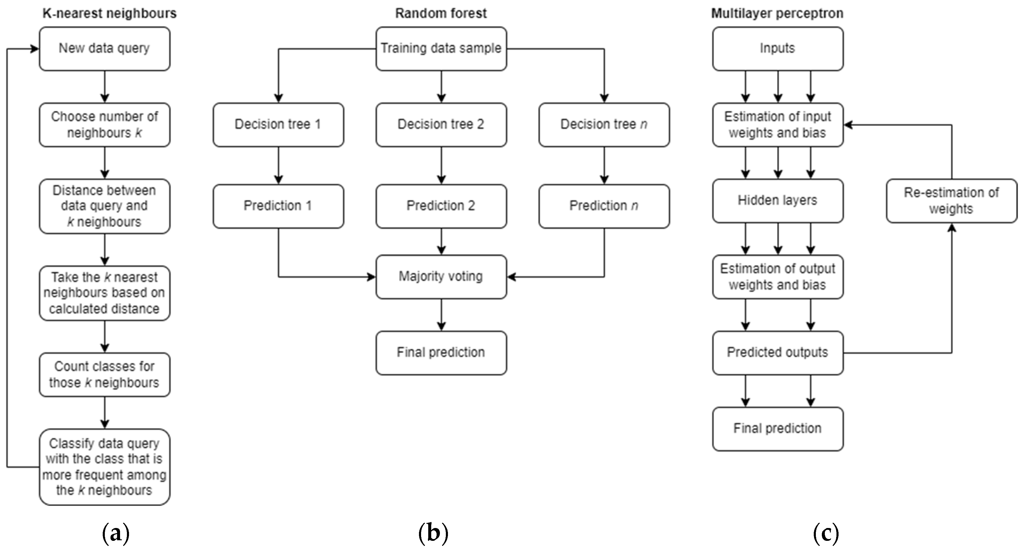
2.2.1. K-Nearest Neighbors

This classification algorithm is fundamentally simple but exhibits relative high performance. The underlying intuition is based on classifying the information from specific features from the categories of its closest neighbors [46]. The number of neighbors ($k$) can be user-defined or it can vary depending on the local density of the neighborhood. Likewise, to quantify the proximity of such neighbors, different measures of distance can be used, such as Euclidean or Manhattan distance. The distance from a close neighbor can also be weighted so that it provides a higher influence than a farther one.

Major limitations of this algorithm are its lack of performance when dealing with high-dimensional data and its high prediction times for large datasets. The reader is referred to [47] for a deeper description of this algorithm.

2.2.2. Random Forest

The random forest algorithm is based on decision trees, where the data are split into different branches that are created on the basis of specific data subsets. Random forest consists of creating multiple decision trees and randomizing the set of features these trees are fed into [48]. This approach is a trademark for what is known as ensemble learning. The response of each tree is then compared, and, in the case of classification, the mode of the outputs is considered as the categorical prediction. The diverse nature of the random forest algorithm, i.e., the use of multiple classifiers to find a robust prediction, allows for low-variance responses, which is a desired characteristic in any machine learning method [49]. The predictions are also expected to be unbiased.

A particularity of this method is the identification and ranking of the most relevant features in the datasets with respect to the categorical responses. This can be useful as a complement for the study of the effect of single features on the output response.

The main disadvantage of this algorithm is the large computational time required for implementation, which increases with the number of trees to build (defined by the user). More details regarding the algorithm can be found in [50].

2.2.3. Multilayer Perceptron

A multilayer perceptron (MLP) is a type of artificial neural network. It consists of an input layer that receives the data, a set of hidden layers that process the data, and an output layer that contains the response of the classification [49]. The network is trained via backpropagation, which is an optimization technique where a cost function (related to the difference between predictions and true values) is minimized. The function learned by the neural network consists of the linear combination of a set of two parameters, namely, weights and biases. The use of this method allows for flexibility, as linear and nonlinear systems can be fitted to the network and in cases where online predictions are needed.

Major drawbacks of this algorithm are its strong dependence on hyperparameters (i.e., number of neurons, number of hidden layers, etc.) and the presence of local minima when using hidden layers. This means that, when more hidden layers are used to increase accuracy, there is a major risk of deviating from a global optimal solution. A deeper description and the advantages of this algorithm can be found in [51].

3. Results and Discussion

Three different classifiers were built for each of the working fluids (ethanol and FC-72) using the experimental data. These data comprise 9841 observations for ethanol and 8590 observations for FC-72. The input features considered for all classifiers and both working fluids are the modified versions of Weber, Froude, and Bond numbers, represented by $W{e}_l^{*}$, $F{r}_l^{*}$, and $B{o}_l^{*}$, respectively. These numbers were defined using actual bubble lengths, velocities, and accelerations, estimated via specific image analysis methods. More details regarding the definition of each number and data pre-processing can be found in Pietrasanta et al. [29]. The categorical output data indicate whether a specific observation is classified as slug/plug flow or semi-annular flow, and it was conducted visually. For each working fluid and classifier, the steps described below were carried out.

3.1. Data Splitting

Datasets were randomly split into training and testing sets. This was applied to avoid using entire datasets for training stages, as this could lead to overfitting. The proportion of data used in the training stage was fixed to 70%. This proportion of data splitting is commonly used, along with similar splitting ratios such as 80% or 67%. There is no optimal splitting ratio in machine learning applications (in general), and the decision is based on the original datasets. In this work, the datasets for both working fluids were large enough to perform the selected data split, leading to the values presented in

Table 4. Split of data samples for ethanol and FC-722.

Data Sample	Total Data Points	Training Set Data Points	Testing Set Data Points
Ethanol	9841	6888	2953
FC-72	8590	6013	2577

.

3.2. Data Scaling

The values of the input features in the training and testing set were scaled (i.e., normalized) to avoid issues from different orders of magnitude among feature values. This was achieved by estimating the expected value and standard deviation of the training and testing sets and applying the normalization formula shown in Equation (2), where $z_i$ is the normalized data point, $x_i$ is the original data point, $\overline{\mu }$ is the sample’s mean or expected value, and $sd$ is the sample’s standard deviation. The result from this normalization procedure is a transformed dataset that presents an expected value of 0 and a standard deviation of 1.

$$z_i=\frac{x_i-\overline{\mu }}{sd}.$$

(2)

3.3. Classifier Creation

The training set was used to train the classifier and then test it with the testing set. The accuracy score was estimated and stored. At this point, default values for each algorithm’s parameters were used. The selection of the most suitable set of parameters for each method was completed later (see Section 3.6).

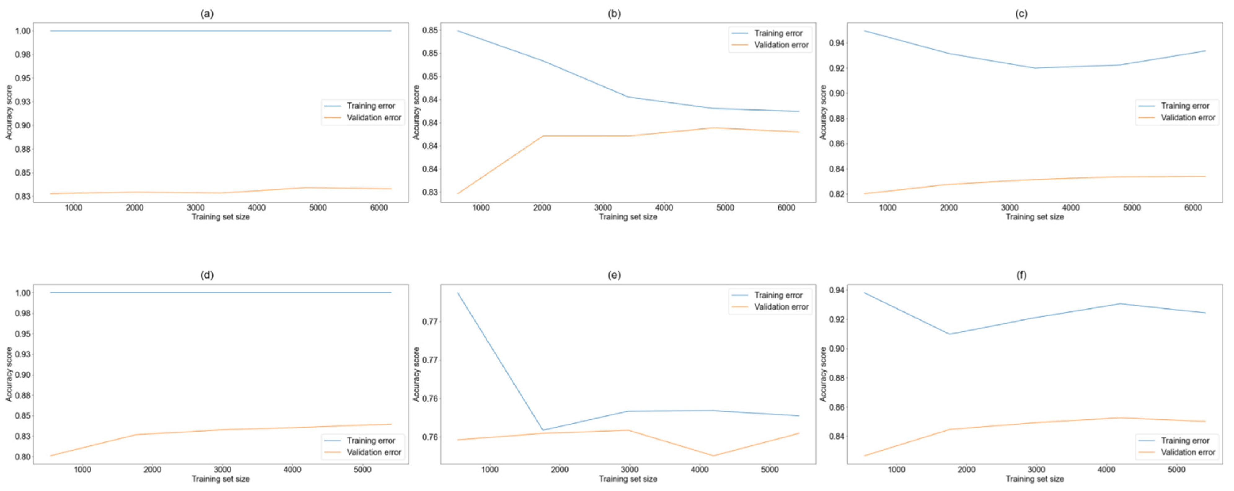
3.4. Cross-Validation

The training set was further used in cross-validation. This method provides a more general indication of the classification performance. In this work, cross-validation was implemented via the so-called k-fold cross-validation method. Here, the training set was further split into k subsets, which were smaller than the training set. This was followed by subsequent trainings of the classification algorithm using k − 1 subsets as the training set, while the remaining data were set aside for testing. The accuracy score was then estimated for all folds and averaged to get a representation of the overall performance of the classifier. This allowed for a higher training/testing split, as a validation set is not necessary when using cross-validation. A schematic of the k-fold method is depicted in Figure 4.

3.5. Accuracy Assessment

The accuracy score of the created classifier and the mean score from the cross-validation procedure were compared to assess the general performance of the classifier. This comparison was only for understanding the robustness of the initial classifier. Normally, large differences are expected, leading to the conclusion that the initial set of parameters for each classifier (among other factors such as split ratio, amount of total data, and/or number of input features) should be adjusted.

3.6. Selection of Hyperparameters

To increase classification performance, and to select the most suitable set of parameters for a fair comparison (i.e., comparing only classifiers presenting maximum accuracy), a deep analysis was carried out. This is achieved using a grid search. This procedure consisted of choosing a combination of various values for specific parameters within a classifier and exhaustively performing a cross-validation for each combination of parameters. The accuracy score for each of these combinations was stored for comparison, and the set of parameters with the best (maximum in this case) output value of accuracy score was chosen. The updated classifier was then tested using the testing set, and a prediction (testing) accuracy score was stored. Note that, in order to apply this procedure to each selected classifier, a set of different hyperparameters was chosen.

Table 5. Selected hyperparameters for grid search and cross-validation procedures.

KNN	Random Forest	MLP
Leaf size	Number of trees in the forest	Maximum number of iterations
Number of neighbors	Criterion for split quality	Number of hidden layers
Distance metric	Criterion for maximum features per split	Activation function
-	Minimum samples to split an internal node	Optimization solver
-	Minimum samples to be at a leaf node	Regularization parameter
-	Bootstrap Boolean (resampling)	Learning rate

shows the parameters, which were selected on the basis of the authors’ criteria and availability within the syntax and structure of the applied algorithms (i.e., Sci-kit learn module in Python).

3.7. Classification Results

Once all classifiers were trained and tested with the default parameters, cross-validation and grid search methods were implemented to select the set of parameters that output the maximum accuracies. On the basis of the list of hyperparameters presented in

Table 6. Optimal hyperparameters for K-nearest neighbors classifier.

Parameter	Value—Ethanol	Value—FC-72
Leaf size	1	1
Number of neighbors	25	26
Distance metric	Manhattan distance	Manhattan distance

, the selected ones for the most accurate classifiers are shown in Table 6,

Table 7. Optimal hyperparameters for random forest classifier.

Parameter	Value—Ethanol	Value—FC-72
Number of trees in the forest	100	100
Criterion for split quality	Entropy	Entropy
Criterion for maximum features per split	Squared root of features	Squared root of features
Minimum samples to split an internal node	10	2
Minimum samples to be at a leaf node	2	2
Bootstrap Boolean (resampling)	True	True

and

Table 8. Optimal hyperparameters for multilayer perceptron classifier.

Parameter	Value—Ethanol	Value—FC-72
Maximum number of iterations	1000	100
Number of hidden layers	2	2
Activation function	ReLU	ReLU
Optimization solver	Adam	Adam
Regularization parameter	0.0001	0.0001
Learning rate	adaptive	adaptive

for the K-nearest neighbors, random forest, and multilayer perceptron, respectively. These classifiers were used for comparing accuracy using the testing set in later stages. Note that these optimal parameters varied when choosing a different working fluid, as the results for ethanol could not be extrapolated to those for FC-72. Nevertheless, slight differences could be seen, especially with those classifiers that do not depend on a large number of hyperparameters, such as the K-nearest neighbors classifier. For this classifier, a training set was split even though it was not strictly needed. This was for the sake of consistency when comparing all three classifiers.

To assess the performance of individual classifiers after identifying the best set of hyperparameters, normalized confusion matrices were used to visualize the distribution of correct and incorrect classifications on the testing set. A confusion matrix depicts the fraction of correct and incorrect labeled points over the total number of true labels. Thus, a matrix entry of 1, for a specific label, indicates that all points in such a dataset are categorized with the expected label. Normalized values were used for more interpretable visual results.

The confusion matrices for the three algorithms in the case of ethanol as the working fluid are shown in

Table 9. Confusion matrix results for ethanol.

		Actual Slug/Plug	Actual Semi-Annular
KNN	Predicted slug/plug	0.89	0.32
	Predicted semi-annular	0.11	0.68
Random Forest	Predicted slug/plug	0.88	0.32
	Predicted semi-annular	0.12	0.68
MLP	Predicted slug/plug	0.90	0.30
	Predicted semi-annular	0.10	0.70

. In general, all algorithms performed similarly, where the classification of slug/plug flow was significantly higher than that of semi-annular flow. This could be due to the increase in observation errors while classifying semi-annular flow or to the innate nature of this flow pattern, which could have led to more erroneous observations.

In the case of ethanol, the multilayer perceptron exhibited a slightly higher number of correct classifications, considering both slug/plug and semi-annular flow. These low differences among the three classifiers suggest that, given the available data and selected input features (limited by design and, thus, subject to potential improvements), a fixed order of accuracy could be reached by all algorithms, with the highest provided by MLP.

In the case of FC-72, the highest fraction of correct classifications was also found using the MLP classifier. The major difference across classifiers was seen in the slug/plug category. The confusion matrices for FC-72 are illustrated in

Table 10. Confusion matrix results for FC-72.

		Actual Slug/Plug	Actual Semi-Annular
KNN	Predicted slug/plug	0.90	0.33
	Predicted semi-annular	0.10	0.67
Random Forest	Predicted slug/plug	0.89	0.34
	Predicted semi-annular	0.11	0.66
MLP	Predicted slug/plug	0.91	0.33
	Predicted semi-annular	0.09	0.67

. As in the case of ethanol, the MLP classifier tended to present the highest accuracy among the algorithms with the testing set, after selecting the most suitable set of hyperparameters.

The overall classification performance is reflected in the value of the accuracy score. These values are reported in

Table 11. Accuracy score for each algorithm: ethanol.

Classifier	Accuracy (%)
K-nearest neighbors	82.8
ANN	83.9
Random forest	82.2

and

Table 12. Accuracy score for each algorithm: FC-72.

Classifier	Accuracy (%)
K-nearest neighbors	75.8
ANN	77.1
Random forest	75.6

, respectively. These values represent the accuracy of those classifiers that presented the highest cross-validated score when selecting the most suitable set of hyperparameters. In accordance with the confusion matrices, the results suggest that the use of MLP provided the highest performance. The lowest performance was shown by the random forest algorithm. In this work, this accuracy score was chosen as a selection criterion for the most suitable classification method; however, it is acknowledged that additional criteria such as computational time or performance when dealing with larger datasets could be included.

An alternative and complementary method for evaluating the performance of each classification algorithm is the analysis of learning curves. A learning curve shows the sensitivity of a particular performance metric (i.e., accuracy score, mean squared error, etc.) with respect to the size of the training set. This allows the user to identify (i) whether it is necessary to include more data samples in the training set, and (ii) whether the classifier under study presents a bias error or a variance one. Generally speaking, a bias error indicates that the classifier could be overly simple/complex with respect to the training set, leading to either overfitting or underfitting cases. Similarly, a variance error indicates that the classifier could vary drastically or remain unaffected when moving from training (seen data) to testing (unseen data). This also leads to overly simplistic/complex models depending on the case [49].

Both these concepts are related, as machine learning models with high/low bias present low/high variance, exhibiting a tradeoff that should always be taken into account [49]. To evaluate this tradeoff in both training and validation stages, the learning curves for each classifier and working fluid were created. Once the hyperparameters of each algorithm were selected via grid search, different sizes of training data were chosen (as a proportion of the initial training set size; see Table 4), and the training accuracy score was estimated for each training set size. For the validation curve, cross-validation was used once again (via k-fold cross-validation, as described in Section 3.5), and, for each training set size, accuracy scores were also calculated. The learning curves for all three algorithms and both working fluids are depicted in Figure 5.

Figure 5 reveals that the training error for the KNN classifier in both working fluids (a and d, respectively) was equal to 1, denoting perfect accuracy. Although this might seem like a successful result, there was a relatively large gap between the training score trend and that for the validation set. This gap is indicative of variance error, as the classifier performed well only during training. The accuracy score in both datasets was within the range of 83% to 100% for both working fluids, suggesting a small bias error in both stages. A similar case was seen in the random forest classifier. However, in this case, the variability of the accuracy score in the training set behaved differently as the size of the training set increased for both working fluids. A minimum accuracy score was reached with ethanol as a working fluid, whereas an oscillating trend was seen when working with FC-72. The accuracy score in the validation set was seemingly improved with the increase in data samples. In general, the random forest algorithm presented a lower bias error than KNN. On the other hand, the MLP classifier presented a smaller gap between training and validation stages, indicating a good balance between variance and bias errors, as the accuracy score for both stages was within the range of 84% to 85%. This suggests that the tradeoff for this method was the most balanced.

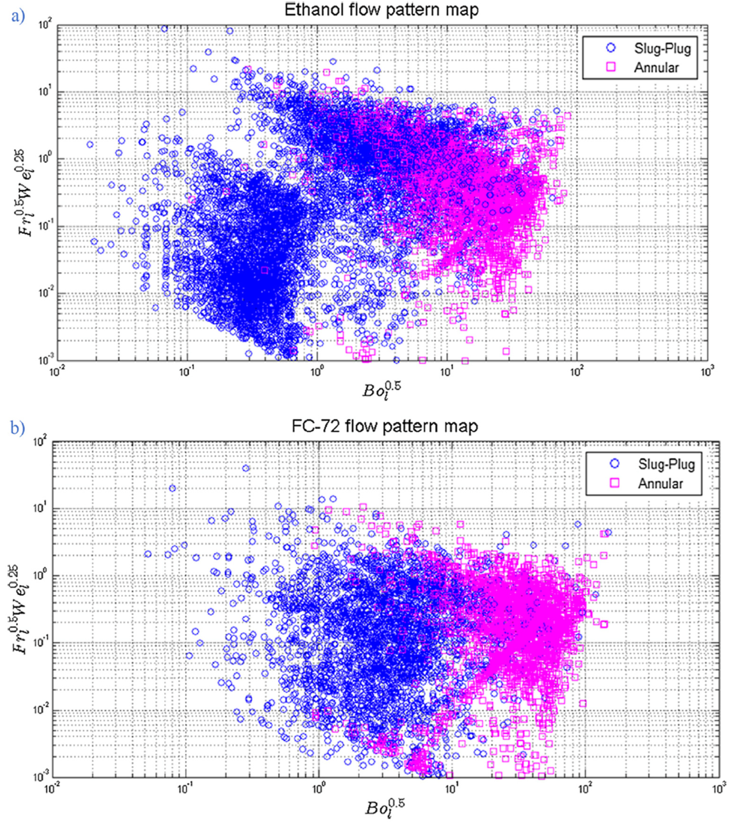
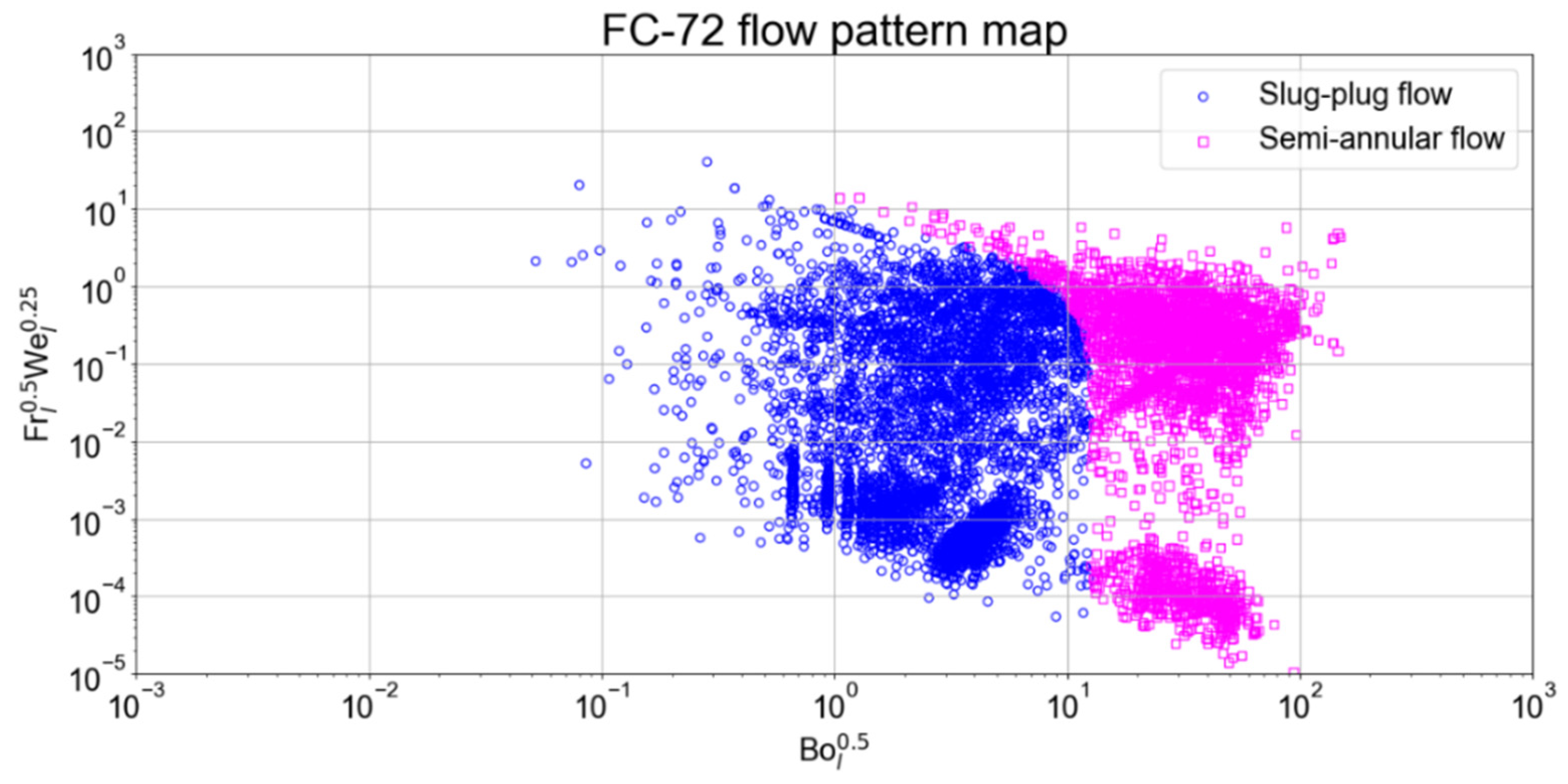
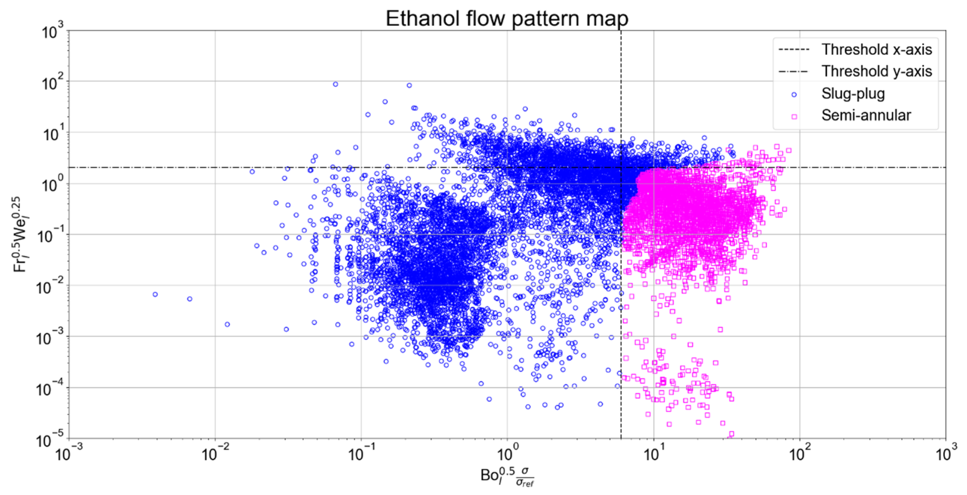
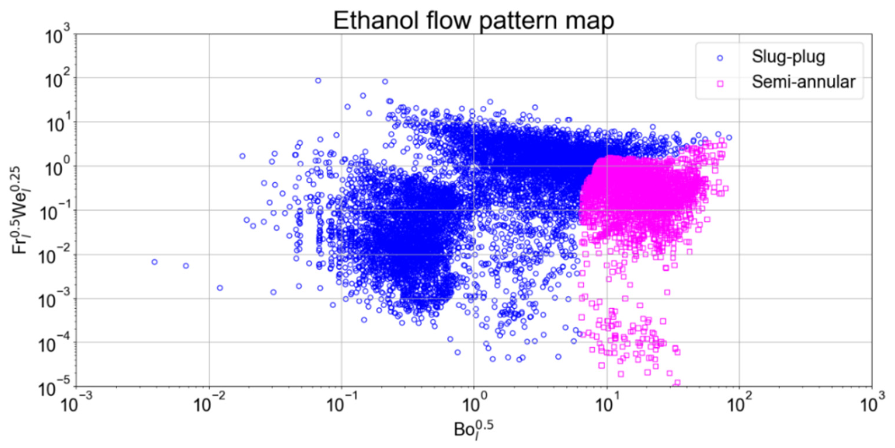
3.8. Flow Pattern Maps

The classification results from the most accurate classifier (MLP in this case) were used to develop a flow pattern map for both ethanol and FC-72. Once the classifier predicted the classes for each data point in the testing set (those in the training set were already stored during training), these points were used to estimate the values for the flow pattern maps. As a result, the maps can be used as a graphic tool for visualizing the outcomes from the classification methods. The x-axis corresponds to $B{o}_l^{0.5}$, and the y-axis corresponds to $F{r}_l^{0.5}W{e}_l^{0.25}$, in accordance with the correlation between process conditions (velocity and acceleration) and the effect of the different forces acting on the fluid (namely, inertial, external, and related to the surface tension) proposed by Pietrasanta et al. [29]. The resulting flow pattern maps for both fluids developed by the authors are illustrated in Figure 6. These maps can act as a reference for comparison with the flow pattern maps from the MLP classifier.

For both working fluids, a much clearer transition zone was found when comparing the previous flow pattern maps and those based on the MLP classifier. This was due to the inherent improvements brought about by the use of the MLP method, as this algorithm provides a more systematic mean for classification compared to visual categorization or empirical correlations with physical properties.

Figure 7 shows the flow pattern map for ethanol. The map clearly shows a threshold value where the transition from slug/plug to semi-annular flow took place, located approximately where the x-axis was equal to 4. Higher values along this axis indicate semi-annular flow, where surface tension no longer dominated the fluid flow, and the increased acceleration led to higher bubble lengths. Semi-annular flow can be further identified on the y-axis, where for values of $F{r}_l^{0.5}W{e}_l^{0.25}$ lower than 2, a relatively high density of points classified as semi-annular flow was encountered. Lower values on both axes indicated the presence of slug-plug flow, either because the PHP device was not active or because the external forces were not strong enough to prevail over the surface tension of the working fluid while operating.

In the case of FC-72, its corresponding flow pattern map is shown in Figure 8. Similar to the case of ethanol, a threshold value for the transition zone was found. Here, the threshold was located approximately when $B{o}_l^{0.5}$ = 9. This means that slug/plug flow prevailed for higher velocities and bubble lengths when FC-72 was used as working fluid. This can be explained by the differences in the surface tension of both fluids. FC-72 has a lower surface tension than ethanol; hence, for the same dynamic conditions (fluid velocity and acceleration), greater numbers of $B{o}_l^{0.5}$ would be reached before the flow regime transition. Abnormal points were found within the slug/plug region for FC-72, which were classified as semi-annular. This phenomenon could have been caused by the propagation of visual errors, as discussed previously. This would also mean that the choice of $B{o}_l$ did not properly reflect the surface tension effects, since this number could not capture the regimes for both fluids.

To overcome the effect of different surface tension in both working fluids, a modified term was used on the x-axis of both flow pattern maps. The term $B{o}_l^{0.5}$ was scaled using the ratio $\frac{{\sigma }_l}{{\sigma }_{ref}}$, where ${\sigma }_l$ represents the surface tension of the working fluid, and ${\sigma }_{ref}$ is a reference surface tension, which in this case was that of ethanol. Surface tension for both fluids was estimated via validated correlations that depend on key operating conditions such as saturation temperature [29]. This correction ratio was calculated for each observation, and updated flow pattern maps for both fluids were developed (using the MLP classifier). Note that, since ethanol was used as reference, no changes were found in its flow pattern map. The updated flow pattern maps for ethanol and FC-72 are depicted in Figure 9 and Figure 10, respectively.

The updated flow pattern maps exhibited more consistent threshold values on both axes, for both working fluids. In the case of ethanol, these values were 6 for the x-axis and 2 for the y-axis, whereas, for FC-72, these limits were located at 5 for the x-axis and 1 for the y-axis. These values allowed for more interpretability, as it was now possible to cluster the observations and determine their corresponding flow regime on the basis of their relative location to the threshold values, with a margin of only $\pm 1$ unit on each axis.

Overall, the predictions presented good correspondence with experimental results, and the use of modified numbers plus scaling allowed for a clearer differentiation of flow regimes. However, it is worth noting that, although a relatively large number of data were used, this only represents a single PHP design (e.g., the single-loop PHP). Therefore, any attempt to implement these classifiers in a different system would most likely provide less accurate predictions, and a more extensive dataset would be needed.

4. Conclusions

For the purpose of proposing accurate data-driven methods for the flow regime classification in PHP systems, three different machine learning algorithms were tested on experimental data from a PHP device, for two different working fluids (namely, ethanol and FC-72). Both datasets were labeled with their corresponding flow regimes, and the most relevant input features were identified and embedded into specific groups of dimensionless numbers that accurately captured the physical phenomena. All three classifiers showed good performance, whereby the classification of the ethanol data was more accurate than that of FC-72, indicating that the process of labeling the data may have been more challenging in the latter case. The use of the multilayer perceptron (MLP) exhibited the highest performance for both working fluids, whereas the random forest algorithm presented the lowest accuracy, although all algorithms performed similarly. The prediction results from the most accurate classifiers were used to build a flow pattern map for each working fluid. In both cases, clear thresholds were identified, where the transition from slug/plug to semi-annular flow took place. These bounds were obtained after scaling the values of the modified Bond number with those of surface tension for both working fluids. The use of a trained and an automatic classifier in this context could provide a more accurate and less demanding classification of flow regimes. Considering a larger set of data with heat fluxes and geometrical parameters, since effective bubble accelerations and velocities would be dependent variables in this case, this method could effectively offer the chance of overcoming the rough use of Bond numbers to predict confined slug/plug flows in PHPs.

Further extensions of this work include the use of more diverse data, which will improve the robustness of the classification algorithms. In addition, the use of unsupervised learning could be a next step and a significant upgrade. In this way, the labeling process would not be needed, and an appropriate algorithm would identify different clusters of data that may correspond with the flow regimes the clusters belong to. Note that the selection of input features is still of great importance, and the use of the modified Weber, Froude, and Bond numbers can be validated from the results of the clustering.

The use of accurate classifiers in this context allows for a more straightforward identification of flow regimes. This enables the correct selection of models to be used for design, simulation, and optimization of PHP systems. Additionally, regression algorithms can be integrated to the current framework to estimate thermal resistance, which would provide a substantial input for estimating the thermal performance of PHP devices. The results can reveal a clear and robust path to define operational regimes in PHP devices. Moreover, the use of more data from other experiments with different geometries, fluids, and materials can provide a useful resource to improve the applicability of classifiers.

References

1. Karthik, C.A.; Kalita, P.; Cui, X.; Peng, X. Thermal Management for Prevention of Failures of Lithium Ion Battery Packs in Electric Vehicles: A Review and Critical Future Aspects. Energy Storage 2020, 2, e137. [Google Scholar] [CrossRef]
2. Feng, X.; Ren, D.; He, X.; Ouyang, M. Mitigating Thermal Runaway of Lithium-Ion Batteries. Joule 2020, 4, 743–770. [Google Scholar] [CrossRef]
3. Jones, N. How to Stop Data Centres from Gobbling up the world’s Electricity. Nature 2018, 561, 163–166. [Google Scholar] [CrossRef] [PubMed]
4. Kandlikar, S.G. Heat Transfer Mechanisms during Flow Boiling in Microchannels. J. Heat Transf. 2004, 126, 8–16. [Google Scholar] [CrossRef]
5. Thome, J.R. Boiling in Microchannels: A Review of Experiment and Theory. Int. J. Heat Fluid Flow 2004, 25, 128–139. [Google Scholar] [CrossRef]
6. Liu, D.; Garimella, S.V. Flow Boiling Heat Transfer in Microchannels. J. Heat Transf. 2007, 129, 1321–1332. [Google Scholar] [CrossRef]
7. Bar-Cohen, A.; Sheehan, J.R.; Rahim, E. Two-Phase Thermal Transport in Microgap Channels—Theory, Experimental Results, and Predictive Relations. Microgravity Sci. Technol. 2011, 24, 1–15. [Google Scholar] [CrossRef]
8. Baldassari, C.; Marengo, M. Flow Boiling in Microchannels and Microgravity. Prog. Energy Combust. Sci. 2013, 39, 1–36. [Google Scholar] [CrossRef]
9. Mahmoud, M.M.; Karayiannis, T.G. Flow Pattern Transition Models and Correlations for Flow Boiling in Mini-Tubes. Exp. Therm. Fluid Sci. 2016, 70, 270–282. [Google Scholar] [CrossRef] [Green Version]
10. Karayiannis, T.; Mahmoud, M. Flow Boiling in Microchannels: Fundamentals and Applications. Appl. Therm. Eng. 2017, 115, 1372–1397. [Google Scholar] [CrossRef]
11. Ahmad, S.W.; Lewis, J.S.; McGlen, R.J.; Karayiannis, T.G. Pool Boiling on Modified Surfaces Using R-123. Heat Transf. Eng. 2014, 35, 1491–1503. [Google Scholar] [CrossRef] [Green Version]
12. Berenson, P. Experiments on Pool-Boiling Heat Transfer. Int. J. Heat Mass Transf. 1962, 5, 985–999. [Google Scholar] [CrossRef]
13. Marto, P.J.; Lepere, V.J. Pool Boiling Heat Transfer from Enhanced Surfaces to Dielectric Fluids. J. Heat Transf. 1982, 104, 292–299. [Google Scholar] [CrossRef]
14. Mudawar, I.; Anderson, T.M. Optimization of Enhanced Surfaces for High Flux Chip Cooling by Pool Boiling. J. Electron. Packag. 1993, 115, 89–100. [Google Scholar] [CrossRef] [Green Version]
15. Estes, K.A.; Mudawar, I. Comparison of Two-Phase Electronic Cooling Using Free Jets and Sprays. J. Electron. Packag. 1995, 117, 323–332. [Google Scholar] [CrossRef]
16. Bintoro, J.S.; Akbarzadeh, A.; Mochizuki, M. A Closed-Loop Electronics Cooling by Implementing Single Phase Impinging Jet and Mini Channels Heat Exchanger. Appl. Therm. Eng. 2005, 25, 2740–2753. [Google Scholar] [CrossRef]
17. Rau, M.J.; Dede, E.M.; Garimella, S.V. Local Single- and Two-Phase Heat Transfer from an Impinging Cross-Shaped Jet. Int. J. Heat Mass Transf. 2014, 79, 432–436. [Google Scholar] [CrossRef] [Green Version]
18. De Oliveira, P.A.; Barbosa, J.R. Novel Two-Phase Jet Impingement Heat Sink for Active Cooling of Electronic Devices. Appl. Therm. Eng. 2017, 112, 952–964. [Google Scholar] [CrossRef]
19. Thome, J.R. Encyclopedia of Two-Phase Heat Transfer and Flow IV; World Scientific Pub Co. Pte. Lt.: Singapore, 2018; Volume 1. [Google Scholar] [CrossRef]
20. Akachi, H. Structure of a Heat Pipe. U.S. Patent 4921041, 1990. Available online: https://patentimages.storage.googleapis.com/pdfs/US4921041.pdf (accessed on 23 October 2020).
21. Akachi, H. Structure of a Micro-Heat Pipe. U.S. Patent US005219020A, 1993. Available online: https://patentimages.storage.googleapis.com/8d/87/57/18fa8dfa9abc67/US5219020.pdf (accessed on 23 October 2020).
22. Das, S.; Nikolayev, V.; Lefevre, F.; Pottier, B.; Khandekar, S.; Bonjour, J. Thermally Induced Two-Phase Oscillating Flow Inside a Capillary Tube. Int. J. Heat Mass Transf. 2010, 53, 3905–3913. [Google Scholar] [CrossRef] [Green Version]
23. Nine, J.; Tanshen, R.; Munkhbayar, B.; Chung, H.; Jeong, H. Analysis of Pressure Fluctuations to Evaluate Thermal Performance of Oscillating Heat Pipe. Energy 2014, 70, 135–142. [Google Scholar] [CrossRef]
24. Nikolayev, V.S. A Dynamic Film Model of the Pulsating Heat Pipe. J. Heat Transf. 2011, 133, 081504. [Google Scholar] [CrossRef]
25. Nekrashevych, I.; Nikolayev, V.S. Effect of Tube Heat Conduction on the Pulsating Heat Pipe Start-up. Appl. Therm. Eng. 2017, 117, 24–29. [Google Scholar] [CrossRef] [Green Version]
26. Nekrashevych, I.; Nikolayev, V.S. Pulsating Heat Pipe Simulations: Impact of PHP Orientation. Microgravity Sci. Technol. 2019, 31, 241–248. [Google Scholar] [CrossRef] [Green Version]
27. Liu, S.; Li, J.; Dong, X.; Chen, H. Experimental Study of Flow Patterns and Improved Configurations for Pulsating Heat Pipes. J. Therm. Sci. 2007, 16, 56–62. [Google Scholar] [CrossRef]
28. Nazari, M.A.; Ahmadi, M.H.; Ghasempour, R.; Shafii, M.B. How to Improve the Thermal Performance of Pulsating Heat Pipes: A Review on Working Fluid. Renew. Sustain. Energy Rev. 2018, 91, 630–638. [Google Scholar] [CrossRef]
29. Pietrasanta, L.; Mameli, M.; Mangini, D.; Georgoulas, A.; Miché, N.; Filippeschi, S.; Marengo, M. Developing Flow Pattern Maps for Accelerated Two-Phase Capillary Flows. Exp. Therm. Fluid Sci. 2020, 112, 109981. [Google Scholar] [CrossRef]
30. Cheng, L.; Ribatski, G.; Thome, J.R. Two-Phase Flow Patterns and Flow-Pattern Maps: Fundamentals and Applications. Appl. Mech. Rev. 2008, 61, 050802. [Google Scholar] [CrossRef]
31. Özdemir, M.R.; Mahmoud, M.M.; Karayiannis, T.G. Flow Boiling of Water in a Rectangular Metallic Microchannel. Heat Transf. Eng. 2021, 42, 492–516. [Google Scholar] [CrossRef] [Green Version]
32. Kandlikar, S.G.; Garimella, S.; Li, D.; Colin, S.; King, M.R. Heat Transfer and Fluid Flow in Minichannels and Microchannels; Elsevier: Amsterdam, The Netherlands, 2006; pp. 175–226. [Google Scholar] [CrossRef]
33. Mameli, M.; Catarsi, A.; Mangini, D.; Pietrasanta, L.; Miché, N.; Marengo, M.; Di Marco, P.; Filippeschi, S. Start-up in Microgravity and Local Thermodynamic States of a Hybrid Loop thermosyphon/Pulsating Heat Pipe. Appl. Therm. Eng. 2019, 158, 113771. [Google Scholar] [CrossRef]
34. Andredaki, M.; Georgoulas, A.; Miché, N.; Marengo, M. Accelerating Taylor Bubbles within Circular Capillary Channels: Break-up Mechanisms and Regimes. Int. J. Multiph. Flow 2020, 134, 103488. [Google Scholar] [CrossRef]
35. Guillen-Rondon, P.; Robinson, M.D.; Torres, C.; Pereya, E. Support Vector Machine Application for Multiphase Flow Pattern Prediction. arXiv 2018, arXiv:1806.05054. [Google Scholar]
36. Zhu, G.; Wen, T.; Zhang, D. Machine Learning Based Approach for the Prediction of Flow boiling/Condensation Heat Transfer Performance in Mini Channels with Serrated Fins. Int. J. Heat Mass Transf. 2021, 166, 120783. [Google Scholar] [CrossRef]
37. Suh, Y.; Bostanabad, R.; Won, Y. Deep Learning Predicts Boiling Heat Transfer. Sci. Rep. 2021, 11, 5622. [Google Scholar] [CrossRef] [PubMed]
38. Hernandez, J.S.; Valencia, C.; Ratkovich, N.; Torres, C.F.; Muñoz, F. Data Driven Methodology for Model Selection in Flow Pattern Prediction. Heliyon 2019, 5, e02718. [Google Scholar] [CrossRef] [PubMed] [Green Version]
39. Zhang, Y.; Azman, A.N.; Xu, K.-W.; Kang, C.; Kim, H.-B. Two-Phase Flow Regime Identification Based on the Liquid-Phase Velocity Information and Machine Learning. Exp. Fluids 2020, 61, 212. [Google Scholar] [CrossRef]
40. Jokar, A.; Godarzi, A.A.; Saber, M.; Shafii, M.B. Simulation and Optimization of a Pulsating Heat Pipe Using Artificial Neural Network and Genetic Algorithm. Heat Mass Transf. 2016, 52, 2437–2445. [Google Scholar] [CrossRef]
41. Jalilian, M.; Kargarsharifabad, H.; Godarzi, A.A.; Ghofrani, A.; Shafii, M.B. Simulation and Optimization of Pulsating Heat Pipe Flat-Plate Solar Collectors Using Neural Networks and Genetic Algorithm: A Semi-Experimental Investigation. Clean Technol. Environ. Policy 2016, 18, 2251–2264. [Google Scholar] [CrossRef]
42. Patel, V.M.; Mehta, H.B. Thermal Performance Prediction Models for a Pulsating Heat Pipe Using Artificial Neural Network (ANN) and Regression/Correlation Analysis (RCA). Sādhanā 2018, 43, 184. [Google Scholar] [CrossRef] [Green Version]
43. Wang, X.; Yan, Y.; Meng, X.; Chen, G. A General Method to Predict the Performance of Closed Pulsating Heat Pipe by Artificial Neural Network. Appl. Therm. Eng. 2019, 157, 113761. [Google Scholar] [CrossRef]
44. Pietrasanta, L.; Mangini, D.; Fioriti, D.; Miché, N.; Andredaki, M.; Georgoulas, A.; Araneo, L.; Marengo, M. A Single Loop Pulsating Heat Pipe in Varying Gravity Conditions: Experimental Results and Numerical Simulations. In Proceedings of the International Heat Transfer Conference 16, Beijing, China, 10–15 August 2018; Volume 16, pp. 4877–4884. [Google Scholar] [CrossRef]
45. Pletser, V. European Aircraft Parabolic Flights for Microgravity Research, Applications and Exploration: A Review. Reach 2016, 1, 11–19. [Google Scholar] [CrossRef]
46. Altman, N.S. An Introduction to Kernel and Nearest-Neighbor Nonparametric Regression. Am. Stat. 1992, 46, 175–185. [Google Scholar] [CrossRef] [Green Version]
47. Duda, R.O.; Heart, P.E.; Stork, D.G. Pattern Classification, 2nd ed.; Wiley-Interscience: Hoboken, NJ, USA, 2000; ISBN 9780471056690. [Google Scholar]
48. Breiman, L. Random Forests. Mach. Learn. 2001, 45, 5–32. [Google Scholar] [CrossRef] [Green Version]
49. Hastie, T.; Tibshirani, R.; Friedman, J. The Elements of Statistical Learning; Springer: Berlin/Heidelberg, Germany, 2009. [Google Scholar] [CrossRef]
50. Geurts, P.; Ernst, D.; Wehenkel, L. Extremely Randomized Trees. Mach. Learn. 2006, 63, 3–42. [Google Scholar] [CrossRef] [Green Version]
51. Pal, S.; Mitra, S. Multilayer Perceptron, Fuzzy Sets, and Classification. IEEE Trans. Neural Networks 1992, 3, 683–697. [Google Scholar] [CrossRef]
Figure 1. Flow patterns observed in the adiabatic section of a 1.6 mm ID PHP filled with ethanol during a series of experiments [9]. S: slug/plug; SA: semi-annular; A: annular.
Energies 15 01970 g001
Figure 2. Rendering of the single-loop PHP with position of sensors and camera [45]. Reproduced with permissions.
Energies 15 01970 g002
Figure 3. Schematics of selected classification algorithms. (a): K-nearest neighbors, (b): random forest, (c): multilayer perceptron.
Energies 15 01970 g003
Figure 4. The k-fold cross-validation procedure with n folds.
Energies 15 01970 g004
Figure 5. Training and cross-validation curves: (a) KNN with ethanol; (b) MLP with ethanol; (c) random forest with ethanol; (d) KNN with FC-72; (e) MLP with FC-72; (f) random forest with FC-72.
Energies 15 01970 g005
Figure 6. Flow pattern maps for ethanol (a) and FC-72 (b) proposed by Pietrasanta et al. [29]. Reproduced with permissions.
Energies 15 01970 g006
Figure 7. Flow pattern map for ethanol: multilayer perceptron.
Energies 15 01970 g007
Figure 8. Flow pattern map for FC-72: multilayer perceptron.
Energies 15 01970 g008
Figure 9. Updated flow pattern map for ethanol: multilayer perceptron.
Energies 15 01970 g009
Figure 10. Updated flow pattern map for FC-72: multilayer perceptron.
Energies 15 01970 g010