Multi-Objective Optimal Integration of Solar Heating and Heat Storage into Existing Fossil Fuel-Based Heat and Power Production Systems

Abstract

Increasing the share of Renewable energy sources in District Heating (DH) systems is of great importance to mitigate their CO₂ emissions. The combined integration of Solar Thermal Collectors (STC) and Thermal Energy Storage (TES) into existing Combined Heat and Power (CHP) systems can be a very cost-effective way to do so. This paper aims at finding the optimal design of STC and TES systems integrated in existing CHP’s considering two distinct objectives: economic profitability and environmental impact. To do so, we developed a three-stage framework based on Pareto-optimal solutions generated by multi-objective optimization, a Technique for Order Preference by Similarity to Ideal Solution (TOPSIS)-entropy method to select the optimal solution, followed by the definition of final Operation strategy. We proposed relevant improvement of the state-of-the-art models used in similar analysis. We also applied the proposed methodology to the case of a representative, 12 MW_th CHP plant. Our results show that, while the addition of TES or STC alone results in limited performances and/or higher costs, both the cost and the CO₂ emissions can be reduced by integrating the optimal combination of STC and TES. For the selected, optimal solution, carbon emissions are reduced by 10%, while the Annual Total Cost (ATC) is reduced by 3%. It also improves the operational flexibility and the efficiency by peak load shaving, load valley filling and thus by decreasing the peak load boiler operation. Compared to the addition of STC alone, the use of TES results in an increased efficiency, from 88% to 92%. The optimal share of STC is then increased from 7% to 10%.

1. Introduction

The share of Renewable Energy Sources (RES) in energy systems is growing rapidly to accelerate the energy transition and tackle climate change. However, their penetration in the heating and cooling sector, which accounts for more than 50% of the final energy demand in EU [1], is only about 22% in Europe [2]. One of the key solutions to increase this share on the short term and in a cost-effective way is to integrate renewable energy in existing District Heating (DH) systems. Many initiatives are currently taken to do so. According to IRENA [3], Denmark has the ambition to increase the share of RES in their DH systems up to 73% in 2030 (vs. 42% in 2014). China targets a 24% share by 2030.

In terms of renewable resources, biomass, solar heating and geothermal energy are the options with largest potential to reach higher shares of RES in DH’s [3], also at large scale [4,5,6]. Among these options, solar collectors present the additional challenge of being an intermittent source of energy, therefore potentially requiring additional heat storage, which represents an interesting optimization problem.

Hot water Thermal Energy Storage (TES) can provide load shifting and is 100 times cheaper than electricity storage for the same energy capacity [7]. Thanks to TES, up to 25% RES would be integrated in energy systems without significantly affecting its efficiency [8]. Hybrid systems composed of Combined Heat and Power (CHP) units integrated with RES and TES is therefore considered as a first step towards the 4th generation district heating systems [8].

TES alone can also be added to existing CHP’s. It contributes to peak load shaving, it can store energy when the demand is low and deliver it when the demand is high. With an optimal operation, it can also increase the energy efficiency, which in turn results in lower CO₂ emissions [9]. In many studies, the optimization of a combined CHP-TES system often focuses on economic aspects, taking into account the cost of CO₂ emissions. Benalcazar [10] proposed an optimization method based on the economic performance for the optimal sizing of how water TES, integrated in an existing CHP plant considering specific investment cost and different carbon prices. His analysis showed that the integration of the TES units can save operational cost and decrease the use of the heat-only boiler, which reduces fuel consumption and decreases CO₂ emissions. Mugnini et al. [11] assessed possible energy flexibility strategies to improve the performance of such system. Their results revealed that a hot water tank can increase the CHP working hours and primary energy savings. Lai et al. [12] developed an operation optimization model based on Particle swarm optimization method, to investigate the flexibility and thermodynamic performance of a CHP unit integrated with an integrated heat storage tank. Their results show that such an integration led to an increased range of operational conditions of CHP units.

Although the addition of Solar Thermal Collectors (STC) can lead to larger CO₂ emission savings than TES alone, they generally increase the production costs of existing systems [3]. The question of the optimal combination of STC and TES in terms of both economic and environmental impacts may therefore be raised. This corresponds to a multi-objective optimization problem with two design variables, i.e., the sizes of the STC and the TES systems.

Single economic objective optimization does not provide alternative solutions to deal with conflicting objectives [13]. Therefore, recent research efforts focused on multi-objective optimization of energy systems. Multi-objective optimization is used to find a trade-off between two or more conflicting objectives to support decision making. Ren et al. [14] proposed a multi-objective linear programming method for operational strategy of a Distributed Energy System (DES). Their model was based on trade-off analysis of economic and environmental optimization. Fazlollahi et al. [15] developed a multi-objective, multi-period optimization for sizing and operating a DH system with the objectives of maximizing the system efficiency and minimizing the CO₂ emissions and the Annual Total Cost (ATC), the annualized value of the total cost over the lifetime of the project. Luo et al. [16] developed a framework for the optimization of DES integrated with Genetic Algorithm for multi-objective optimization, and multi-criteria evaluated by Technique for Order Performance by Similarity to an Ideal Solution (TOPSIS) method. Karmellos et al. [17] presented a multi-objective Mixed-integer linear programming (MILP) model for the optimal design and operation of DES by ε-constraint method, with minimizing the ATC, and the total carbon emission as objective function. Franco and Versace [18] carried out a multi-objective strategy considering energetic and economic objectives to investigate design and operation strategy of a CHP-TES to DH network.

As discussed above, various approaches have therefore been applied to determine the economically and/or environmentally optimal design and operation of RES and TES integrated into existing CHP systems. However, the proposed methodologies can be further improved in the following respects. First, the modelling of the CHP systems could be more accurate. An increased accuracy of the techno-economic models for the following aspects could lead to more accurate results [19]: Piece-wise Linear Investment functions allowing for a non-linear evolution of the investment costs, and account for part-load efficiencies, start-up costs, CHP acceptable operation ranges and maximum ramp rates, which significantly affect technical and economic performances. Secondly, few recent works [15,16] integrated multi-objective optimization models with decision making methods to optimize the capacity and the operation strategy of TES and RES integrated to existing CHP systems. Moreover, limited research was carried out on the effect of fluctuating investment cost on the sizing and the operation of the system.

In this work, we therefore aim at integrating multi-objective optimization and decision-making methods featuring advanced techno-economic models, and to apply them to 1the STC and TES systems.

Our main objectives are the development a comprehensive methodology to allow decision-makers to determine the optimal design of hybrid heat and power production systems and to assess the economic and environmental impact of the optimal integration of STC and TES systems into existing, conventional CHP systems.

The main innovative features of this work can be summarized as follows:

• The techno-economic models of the sub-systems features Piece-Wise Linear Investment function, part-load efficiencies, start-up costs, maximum ramp rates and CHP acceptable operation ranges.
• The variation of the economic and technical parameters, such as ambient temperature, electricity and fuel prices, is considered.
• Pareto-optimal solutions are generated using multi-objective optimization, from which the optimal solution is picked using the TOPSIS-entropy method, an effective method to make decisions processes more reliable and accurate.

The paper is organized as follows. Section 2 describes the proposed methodologies. The case of a hybrid energy system is defined in Section 3, including the input data and the investigated scenarios. Section 4 presents and discusses the results of the case study. Lastly, conclusions are drawn in Section 5.

2. Materials and Methods

This Section describes the proposed methodology for the optimization of the studied hybrid systems. Their general structure is defined in Section 2.1. The multi-objective optimization model is then described in Section 2.2. Finally, the Decision-making method is presented in Section 2.3.

Figure 1 illustrates the flow chart of the optimization framework used in this study. The framework consists of three stages:

• Pareto-optimal solutions, generated by multi objective optimization model. It involves a trade-off analysis between economic and environmental aspects.
• Optimal solution selected among the Pareto solutions using a decision-making tool. The optimal solution with the maximum relative quality ranking is picked up as the final optimal solution.
• Final design and operation strategy. The hourly operation strategy of the optimal solution is further described to assess performance of each unit with optimal capacity. More detailed description will be introduced in the Section 2.2.

2.1. Hybrid Heat and Power Production System

The components of the existing CHP system considered in this study are a 12 MW_th coal-fired CHP with Extraction Condensing (EC) steam turbine, and two gas-fired Heat Only Boilers (HOB) with a thermal power of 5 MW_th, respectively, also connected to the system. The sizes of the STC and of the TES that will be added to the existing system are the design variables. A schematic of the system is given in Figure 2. Electricity is produced by the CHP and sold to the local market. The generated heat can be sent to both the heat clients and the TES system. HOBs are only in operation when the heat production is insufficient. The constraints related to each unit described in Section 2.2.2, and the input data described in Section 3.1.

2.2. Optimization Model

2.2.1. Objective Function

In this study, the weighting method [20] will be used to solve the multi-objective optimization problem through MILP method. The two objective functions to be minimized are the ATC and the total carbon emissions. A general objective function is then defined as shown in Equation (1):

$$min \left\{F_{obj}=\alpha ·\frac{ATC}{AT{C}_{min}}+\left(1-\alpha \right)·\frac{Carbon}{Carbo{n}_{min}}\right\}$$

(1)

where α is a weighting factor and where the objectives functions are normalized using the corresponding single optimization value $AT{C}_{min}$ and $Carbo{n}_{min}$.

The ATC of the studied hybrid systems is defined in Equation (2) as the sum of the annualized investment cost C_inv, the maintenance cost C_M and the operating cost C_O, minus the revenues R_S from the electricity production [14]. The total CO₂ emissions are calculated for all heat and power generation systems by multiplying the fuel consumption with the corresponding CO₂ emission factor, as shown in Equation (3).

$$ATC=C_{inv}+ C_M+C_O-R_{S }$$

(2)

$$Carbon= {\displaystyle \sum }_u{\displaystyle \sum }_{t}C{F}_u\ast F{C}_{u,t}$$

(3)

The total investment cost $C_{inv}$ is calculated following Equation (4). The annualized investment cost $c_{u,t}^{inv}$, $c_t^{invTES}$ and $c_t^{invSTC}$ (Equations (5)–(7)) are calculated using the annuity factor defined in Equation (8), which considers the discount rate $i$ and the lifetime $n_u$ for each unit, respectively. The maintenance costs are defined as a fixed proportion of the investment costs and are calculated following the same structures, see Equation (9). Operational costs consist of fuel consumption and unit startup costs, see Equation (10).

$$C_{inv}={\displaystyle \sum }_u{\displaystyle \sum }_t(c_{u,t}^{inv}\ast Ca{p}_u+c_t^{invTES}\ast V+c_t^{invSTC}\ast A)$$

(4)

$$c_{u,t}^{inv}=\frac{a_u\ast I_u^{inv}}{8760}$$

(5)

$$c_t^{invTES}=\frac{a_u\ast I^{invTES}}{8760}$$

(6)

$$c_t^{invSTC}=\frac{a_u\ast I^{invSTC}}{8760}$$

(7)

$$a_u=\frac{i\ast {\left(1+i\right)}^{n_u}}{{\left(1+i\right)}^{n_u}-1}, \forall \mathrm{u}\in \mathrm{units},\hspace{1em}\mathrm{t} \in \mathrm{periods}$$

(8)

$$C_M={\displaystyle \sum }_u{\displaystyle \sum }_t \left(c_{u,t}^M\ast Ca{p}_u+c_t^{MTES}\ast V+c_t^{MSTC}\ast A\right)$$

(9)

$$C_O={\displaystyle \sum }_u{\displaystyle \sum }_t(c_{u,t}^{fuel}\ast F{C}_{u,t}+{\delta }_{u,t}^{}\ast S{C}_u)$$

(10)

The revenues $R_S$ consist in selling electricity to the grid, see Equation (11).

$$R_S={\displaystyle \sum }_{t}P\ast E{l}_t$$

(11)

2.2.2. Constraints for System Design and Operation

All units are subject to some constraints. The following constraints are considered in this study for the design and the operation of each sub-system.

Common Types of Constraints

Common types of constraints are applied to all units:

• Minimum and maximum loads

For all units, the production must be within the minimum and maximum loads, see Equation (12):

$$PL{R}_{u,t}^{lb}\ast Q_u^{norm} \le Q_{u,t }\le PL{R}_{u,t}^{ub}\ast Q_u^{norm}\hspace{1em}\forall \mathrm{u}\in \mathrm{units},\hspace{1em}\mathrm{t} \in \mathrm{periods}$$

(12)

• Ramping rate limits

Maximum ramping rates (up and down) of the thermal units should be defined for stability, integrity and safety reasons, see Equation (13) and (14):

$$Q_{u,t+1 }-Q_{u,t}\le ram{p}_{{up}_{u,t}}\ast Q_u^{norm}\hspace{1em}\forall \mathrm{u}\in \mathrm{units}, \mathrm{t} \in \mathrm{periods}$$

(13)

$$Q_{u,t+1 }-Q_{u,t}\le ram{p}_{{down}_{u,t}}\ast Q_u^{norm}\hspace{1em}\forall \mathrm{u}\in \mathrm{units}, \mathrm{t} \in \mathrm{periods}$$

(14)

• State of units

In the framework of MILP optimization, the binary variable $I_{u,t}^{use}$ is used to illustrate the state of the units. It is constrained by the variables $T_{u,t}^{ON}$ and $T_{u,t}^{OFF}$ defining whether the unit is on or off at time t, see Equations (15) and (16).

$$I_{u,t+1}^{use}-I_{u,t}^{use} \le T_{u,t+1}^{ON}\hspace{1em}\forall \mathrm{u}\in \mathrm{units}, \mathrm{t} \in \mathrm{periods}$$

(15)

$$I_{u,t}^{use}-I_{u,t+1}^{use}+T_{u,t+1}^{ON}\le T_{u,t+1}^{OFF}\hspace{1em}\forall \mathrm{u}\in \mathrm{units}, \mathrm{t} \in \mathrm{periods}$$

(16)

• Minimum uptime and downtime

Minimum uptime and downtime constraints are considered for safety and reliability reasons. If a unit is in service, the duration should be at least equal to the defined minimum uptime, as indicated in Equation (17). Similarly, if a unit is not in running, the period should be at least equal to the defined minimum downtime as expressed in Equation (18).

$${\displaystyle \sum }_{t-min\_uptime}^t{T}_{u,t}^{ON} \le I_{u,t}^{use}\hspace{1em}\forall \mathrm{u}\in \mathrm{units}, \mathrm{t} \in \left(min\_uptime, \mathrm{periods}\right),$$

(17)

$${\displaystyle \sum }_{t-min\_downtime}^t{T}_{u,t}^{OFF} \le 1-I_{u,t}^{use}\hspace{1em}\forall \mathrm{u}\in \mathrm{units}, \mathrm{t} \in \left(min\_downtime, \mathrm{periods}\right),$$

(18)

Extraction Condensation CHP Unit

The CHP plant considered in this study is of the Extraction Condensation type (EC): heat is provided to the heat clients through the condensation of steam extracted from the turbine. EC-based CHP can be operated in a flexible way, since steam can usually be extracted from more than one pressure stage, and power may vary with same heat production. In this study, the total energy efficiency of the CHP plant is considered as constant, as suggested in [17,19].

For EC-based CHP’s, the power loss coefficient β, defined as the power generation reduction caused by heat extraction, is a key characteristic [21]. It can be calculated based on the ambient and DH temperatures [22], see Equations (19) and (20):

$$\beta =1-\frac{T_0}{T_M}$$

(19)

$$T_M=\frac{T^{supply}-T^{return}}{\ln \left(\frac{T^{supply}}{T^{return}}\right)}$$

(20)

The acceptable operation zone of the CHP plant in terms of heat extraction and electrical power for a given supply and return temperature is illustrated in Figure 3. It is elaborated as suggested by [22]. The blue line BC is the backpressure line, exhibiting a slope σ. It represents the operation points with the designed power to heat ratio [21]. The maximum load line CD is parallel to the minimum load line AB (both with a slope β). Any line with the same slope corresponds to a constant fuel consumption.

Equation (21) and (22) express the corresponding constraints on the operational loads. The fuel consumption can be calculated using Equation (23).

$$P_t^{EC}=PL{R}_t^{EC}\ast I_{EC,t}^{use}\ast \left({\sigma }^{EC}+{\beta }_t\right)\ast Q_{EC}^{norm}-Q_t^{EC}\ast {\beta }_t\hspace{1em}\forall \mathrm{t} \in \mathrm{periods}$$

(21)

$$P_t^{EC}\ge {\sigma }^{EC}\ast Q_t^{EC}\hspace{1em}\forall \mathrm{t} \in \mathrm{periods}$$

(22)

$$F{C}_t^{EC}=(Q_t^{EC}+P_t^{EC})/{\eta }_{EC}\hspace{1em}\forall \mathrm{t} \in \mathrm{periods}$$

(23)

Heat Only Boiler

The part load efficiency of the gas-fired Heat Only Boiler (HOB) is considered according to the model proposed by [19]. Equation (24) provides an expression for the consumption of the HOB boiler, which leads to the non-linear evolution of its efficiency, as shown in Figure 4.

$$F{C}_t^{HOB}=0.4576\ast Q_{HOB}^{norm}\ast I_{HOB,t}^{use}+0.6599\ast Q_t^{HOB}\hspace{1em}\forall \mathrm{t} \in \mathrm{periods}$$

(24)

Equations (25) and (26) state that the two HOB (HOB1 and HOB2) are only in operation when the heat demand cannot be satisfied by the main steam boiler (peak load), during maintenance or when the demand exceeds the CHP output.

$$Q_t^{EC} \ge I_{HOB1,t}^{use}\ast Q_{CHP}^{norm}$$

(25)

$$Q_t^{EC}+Q_t^{HOB}\ge I_{HOB2,t}^{use}\ast (Q_{CHP}^{norm}+Q_{HOB}^{norm})$$

(26)

Thermal Energy Storage Unit

The Thermal Energy Storage (TES) system is modeled based on the formulation proposed by Wang et al. [23]. Upper and lower boundary conditions are defined for the charging and discharging rates, see Equations (27) and (28). To ensure the availability of the TES, the stored thermal energy at the end of the schedule period is assumed to be equal to its initial value, see Equation (29). The energy balance of the system, taking into account the storage efficiency and the charging and discharging efficiencies, is expressed in Equation (30). The binary variable $z\left(t\right)$ is used to illustrate the TES charging and discharging operation status, see Equation (31). Equations (32) and (33) express the constraints that the stored thermal energy must be lower than the maximum storage capacity of the system, which depends on TES volume and DH supply and return temperatures.

$$0\le H{S}_t^{chr} \le {\alpha }_t^{chr}· Ca{p}_t^{TES}\hspace{1em}\forall \mathrm{t} \in \mathrm{periods}$$

(27)

$$0\le H{S}_t^{dis} \le {\alpha }_t^{dis}· Ca{p}_t^{TES}\hspace{1em}\forall \mathrm{t} \in \mathrm{periods}$$

(28)

$$Q_1^{TES}=Q_{end}^{TES}\hspace{1em}\forall \mathrm{t} \in \mathrm{periods}$$

(29)

$$Q_{t }^{TES}={\eta }_s^{TES}{Q}_{t-1}^{TES}+{\eta }_{chr}^{TES}H{S}_t^{chr}-H{S}_t^{dis}/{\eta }_{dis}^{TES}\hspace{1em}\forall \mathrm{t} \in \mathrm{periods}$$

(30)

$$z\left(t\right)=\left\{\begin{array}{cc}1,& H{S}_t^{dis}=0\\ 0,& H{S}_t^{chr}=0\end{array}\right.\hspace{1em}\forall \mathrm{t} \in \mathrm{periods}$$

(31)

$$Ca{p}_t^{TES}=\frac{\rho Vc}{3600}\{\min ((T_t^{supply}-5),98)-\left(T_t^{return}+5\right)\}\hspace{1em}\forall \mathrm{t} \in \mathrm{periods}$$

(32)

$$Q_{t }^{TES}\le Ca{p}_t^{TES}\hspace{1em}\forall \mathrm{t} \in \mathrm{periods}$$

(33)

The investment costs for the TES system, including the auxiliary equipment, can be estimated following [10,24]. Due to limitation of linear programming method, the exponential decay function of specific investment cost should be replaced with piecewise linear approximation for further use [10]. The specific investment costs curve according to [24], a piecewise linear function is used to make it compatible with MILP, see in Figure 5.

Solar Thermal Collectors Unit

Equations (34) shows how the heating performance of STC can be calculated based on the collector area, solar irradiance and DHN temperature according to the formulation from [25].

$$\begin{array}{c}{Q}_t^{STC}=A\ast ((0.839\ast Q_t^{SR}-2.46\ast \left(T_t^{aver}-T_t^{ambient}\right)\\ -0.0197\ast {\left(T_t^{aver}-T_t^{ambient}\right)}^2)\hspace{1em}\forall \mathrm{t} \in \mathrm{periods}\end{array}$$

(34)

The specific investment costs of ground mounted solar collector field (shown in Figure 6a) are estimated based on [25]. PLI is also applied, cumulative investment cost see Figure 6b.

Energy Balance

Equation (35) expresses that the heat demand from the local distribution network must always be fulfilled for each time interval.

$$Q_t^{CHP}+Q_t^{HOB}+Q_t^{STC}+{\eta }_{dis}^{TES}H{S}_t^{dis}-H{S}_t^{chr} \ge Q_t^{demand}\hspace{1em}\forall \mathrm{t} \in \mathrm{periods}$$

(35)

2.3. Decision-Making Method

Figure 7 illustrates the flow chart of the decision-making process used in this study. The decision-making process is to provide a quantitative evaluation on the system with several conflicting objectives, to support the Decision makers the most potential solutions by considering the important criteria [13]. To evaluate performance of the multi-objective optimization model, a decision-making method combining Technique for Order Preference by Similarity to Ideal Solution (TOPSIS) with Entropy method (EM) is investigated. TOPSIS is a classic method to find optimal solution within finite objectives [26], while EM aims at determining the weights of each objective in an automatic way, in order to minimize man-made error [27]. As illustrated in Figure 7, The TOPSIS-entropy method selects the solution with the maximal relative quality as the optimal solution.

The different steps followed to the TOPSIS-entropy method are as follows [28]:

• Weights calculation:

The first step is matrix normalization, see Equation (36). This ensures that all indicators are positive and present comparable ranges. Then, standardized value $p_{ij}$ and entropy value of objective $e_j$ are calculated using Equations (37) and (38). Finally, weighting values of the objectives ${\omega }_j$ are defined, see Equation (39).

$$y_{ij}=\frac{\max \left(x_{ij}\right)-x_{ij}}{\max (x_{ij})-\min \left(x_{ij}\right)}\hspace{1em}\forall \mathrm{i} \in \left[1\dots m\right], \mathrm{i} \in \left(1\dots \mathrm{n}\right)$$

(36)

$$p_{ij}=\frac{y_{ij}}{\sqrt{{{\displaystyle \sum }}_{i=1}^m{y}_{ij}}}\hspace{1em}\forall \mathrm{i} \in \left[1\dots m\right], \mathrm{i} \in \left(1\dots \mathrm{n}\right)$$

(37)

$$e_j=-\frac{1}{\ln \left(m\right)} {{\displaystyle \sum }}_{i=1}^m p_{ij}\ln \left(p_{ij}\right)\hspace{1em}\forall \mathrm{j} \in \left(1\dots \mathrm{n}\right)$$

(38)

$${\omega }_j=\frac{1-e_j}{{{\displaystyle \sum }}_{j=1}^n \left(1-e_j\right)}$$

(39)

• TOPSIS method

The weighted matrix used as a basis for the TOPSIS method is described in. Equation (40) The positive ideal solution $V^{+}$ and negative ideal solution $V^{-}$ are then determined using Equations (41) and (42). The distances $D^{+}$ and $D^{-}$ between any evaluated result and the two positive and negative solution $V^{+}$ and $V^{-}$ are calculated using Equations (43) and (44). Finally, the relative quality $C_i$ is defined to compare the distance between any result and the two ideal solutions, see Equation (45). The optimal solution corresponds to the highest value of $C_i$.

$$v_{ij}={\omega }_{ij}\ast y_{ij}\hspace{1em}\forall \mathrm{i} \in \left[1\dots m\right], \mathrm{i} \in \left(1\dots \mathrm{n}\right)$$

(40)

$$V^{+}=\left\{\left(max V_{ij}|\mathrm{j}\in J_1\right), \left(min V_{ij}|\mathrm{j}\in J_2\right)\right\}\hspace{1em}\forall \mathrm{i} \in \left(1\dots \mathrm{n}\right)$$

(41)

$$V^{-}=\left\{\left(min V_{ij}|\mathrm{j}\in J_1\right), \left(max V_{ij}|\mathrm{j}\in J_2\right)\right\}\hspace{1em}\forall \mathrm{i} \in \left(1\dots \mathrm{n}\right)$$

(42)

$$D^{+}=\sqrt{{{\displaystyle \sum }}_{j=1}^n{(V_{ij}-V_j{}^{+} )}^2}\hspace{1em}\forall \mathrm{i} \in \left(1\dots \mathrm{n}\right)$$

(43)

$$D^{-}=\sqrt{{{\displaystyle \sum }}_{j=1}^n{(V_{ij}-V_j{}^{-})}^2}\hspace{1em}\forall \mathrm{i} \in \left(1\dots m\right)$$

(44)

$$C_i=\frac{D^{-}}{D^{+}-D^{-}}\hspace{1em}\forall \mathrm{i} \in \left(1\dots m\right)$$

(45)

3. Case Study

In this Section, the proposed optimization framework is applied to a specific case of hybrid system described in Section 2.1. The considered input data is described in Section 3.1. Four different scenarios are defined in Section 3.2.

3.1. Input Data

The considered heat demand, ambient temperature, supply and return temperatures are field data retrieved in 2017 from an existing DH plant located in France. The hourly market electricity price was imported from EPEX SPOT for the year 2017 [29] and local climate data of solar radiation were retrieved from PVGIS for the same year [30]. The impact of the uncertainty on the main parameters will be investigated in Section 4.4.

However, the annual profile with 8760 time steps makes is difficult to solve due to complexity of optimization model [31,32,33]. To limit the computational time without significantly impacting the simulation results [32], the approach of typical periods is used in this work [33], a full year period was discretized into 12 typical days, each of them being representative for a month.

Figure 8 shows that the heat demand varies from 1.44 MW_th to 16.9 MW_th. The average heat load and heat load variations are larger in the winter. The corresponding supply and return temperatures range from 75 to 90 ℃ and from 55 to 75 ℃, respectively. The average electricity price is also slightly higher in the winter, as illustrated in Figure 9. For each typical day, the heating load peak is observed between 8 and 10 AM and between 8 and 10 PM, while the peak of electricity price is observed between 8 and 9 AM and between 6 and 7 PM. The hourly variations of ambient temperature and solar irradiance are also presented in Figure 10. The heat collected by the STC was calculated following the methodology of Schmidt (Ref. [10]). The considered tilt angle of the collector was 40°.

The considered technical parameters of the heating and the thermal storage systems are provided in

Table 1. Technical parameters of each unit.

Units	Capacity	Minimum Part Load Ratio	Min Uptime	Min Downtime	Ramp-Up Rate %/h	Ramp-Down Rate %/h	Norm Efficiency
CHP	12 MW	0.3	10	7	30	30	0.883
HOB1	5 MW	0.3	2	2	100	100	0.9
HOB2	5 MW	0.3	2	2	100	100	0.9
TES	0–6000 m3	0	4	4	100	100	-
STC	0–40,000 m2	0	1	1	100	100	-

and

Table 2. Technical parameters of TES [23].

Unit	Charging Ratio	Discharging Ratio	Storage Efficiency per Hour	Charging Efficiency	Discharging Efficiency
TES	0.4	0.4	0.998	0.95	0.95

. The related economic parameters, including investment and maintenance costs, lifetime and startup costs are presented in

Table 3. Economic data of each unit [34].

Units	Investment Cost	Maintenance Cost	Startup Cost per Time	Lifetime
CHP	1154 €/kW	43.2 €/(kW·year)	5000 €	25
HOB	62.9 €/kW	1.26 €/(kW·year)	1290 €	17
TES	See Figure 5	-	-	25
STC	See Figure 6	-	-	30

. The startup costs actually vary with the size of the units, but the constant values from [34] were considered here as they match the considered range of unit size.

CO₂ emissions are calculated based on the specific emission factors to the primary consumption [1]: 350 kg CO₂/MWh for coal and 200 kg CO₂/MWh for natural gas [35]. The CO₂ price in France in 2017 is collected from World Bank Carbon Pricing dashboard 30.5 € per tonne [36]. The fuel costs are assumed constant: 28 €/MWh for Coal and 32 €/MWh for natural gas [34].

The following assumption were also made on the efficiency of the systems: the effect of incidence angle was neglected in the design of the STC system and the CHP operation efficiency was considered constant.

3.2. Scenarios

Different scenarios are investigated in this study to analyze the impact of the integration of TES and STC systems into the existing CHP system. Scenario 1 covers the operation of the existing system without the addition of TES nor STC. Both systems are then considered and optimized in Scenario 2. In Scenarios 3 and 4, the addition of TES or STC alone is studied. The scenarios are summarized in

Table 4. Overview of each Scenario.

Scenario Name	CHP	HOB1	HOB2	TES	STC
1	●	●	●
2	●	●	●	●	●
3	●	●	●	●
4	●	●	●		●

.

4. Results and Discussion

In this Section, the results of the optimization performed for the 4 Scenarios of the case study are presented and discussed. In this study, the MILP model implemented in Python and solved with IBM DOcplex toolbox. Section 4.1 gives the results of the Pareto Frontiers for all Scenarios. In Section 4.2, the optimal solutions chosen using the TOPSIS-entropy method are presented. Section 4.3 gives more detailed information on the hourly operation strategy, and Section 4.4 presents a sensitivity analysis on the main parameters.

4.1. Pareto Frontiers

Figure 11 shows the Pareto frontiers computed for Scenarios 2 to 4 in terms of ATC and CO₂ emissions, expressed relatively to the reference Scenario 1. In Scenario 1, the ATC is 4380 k€/year and the CO₂ emissions are 43,435 ton/year.

Considering the addition of TES only (Scenario 3) quickly allows for a reduction of the system cost (5%) and a moderate reduction of the CO₂ emissions (up to 1% less). This is due to the larger consumption of the produced heat hen heat storage is available (see Section 4.3). When even lower CO₂ emissions must be reached with TES only, the price of the system however increases very sharp: it becomes higher than the reference cost for CO₂ emissions reductions around 7% and increases exponentially afterwards: +30% compared to the reference scenario for a 10% CO₂ emissions reduction.

On the other hand, considering STC only (Scenario 4) immediately leads to a higher cost, because of the higher price of STC. This system however becomes cheaper than TES only to reach CO₂ emissions reductions larger than 8%, although the cost also increases very rapidly for larger emission savings.

Figure 11 also shows that, combining TES and STC (Scenario 2) allows decreasing the ATC while reaching much larger CO₂ emissions reduction. The combination of these systems indeed leads to the valorization of a higher amount of heat collected by the STC system by storing it and making it available when the demand is high. Parity with the reference scenario in terms of costs is reached for 12% less CO₂ emissions. For even lower emissions, the cost increase is also significantly reduced compared to TES or STC only: 17% less CO₂ is emitted for cost increase of 7%. The installation of the additional equipment is made more cost-effective by their complementarity.

4.2. TOPSIS-Entropy Method Analysis

The TOPSIS-entropy method was used to choose the optimal solution on the Pareto frontiers obtained from the MILP optimizations. The weights calculated by the entropy method for each Scenario are very similar: around 0.54 and 0.46 for ATC and CO₂ emissions respectively. The solutions presenting the maximum relative quality for each Scenario are given in

Table 5. Optimal solutions by TOPSIS-entropy method for each scenarios.

Scenario Name	TES/m3	STC/m2	CO2 (ton/year)	ATC (k€/year)	HOB Operation Hour (h/year)	Total Efficiency, %	Share of RES, %
1	-	-	43,435	4380	1520	87	0
2	1382	22,399	39,268	4258	730	92	10
3	742	-	41,184	4198	730	88	0
4	-	17,649	40,363	4471	1460	90	7

and illustrated on the Pareto frontiers of Figure 11. The results generated for 12 representative days, see Section 3.1, have been extrapolated to a full year. Compared to the reference Scenario 1, the identified, optimal solution for Scenario 2 corresponds to a decrease of both the CO₂ emissions (10%) and the ATC (3%), which is an excellent trade-off. The total efficiency of the system increases from 87% to 92%, while the share of renewable energy in the system reaches 10%. The optimal solution for TES only (Scenario 3) is selected before the strong increase of the system cost on the Pareto frontier. The CO₂ emissions are reduced by 5% while the cost is reduced by 4%. When only the STC system is installed (Scenario 4), the optimal solution is again selected before the strong increase of the cost. In that case, the cost increases with 2%, for a CO₂ emissions reduction of 7%. The ATC is higher than for Scenario 2 because of the lower proportion of renewable heat that can be consumed. The addition of TES indeed allows for the displacement of the consumption of the heat collected by the STC to the periods when the demand is higher.

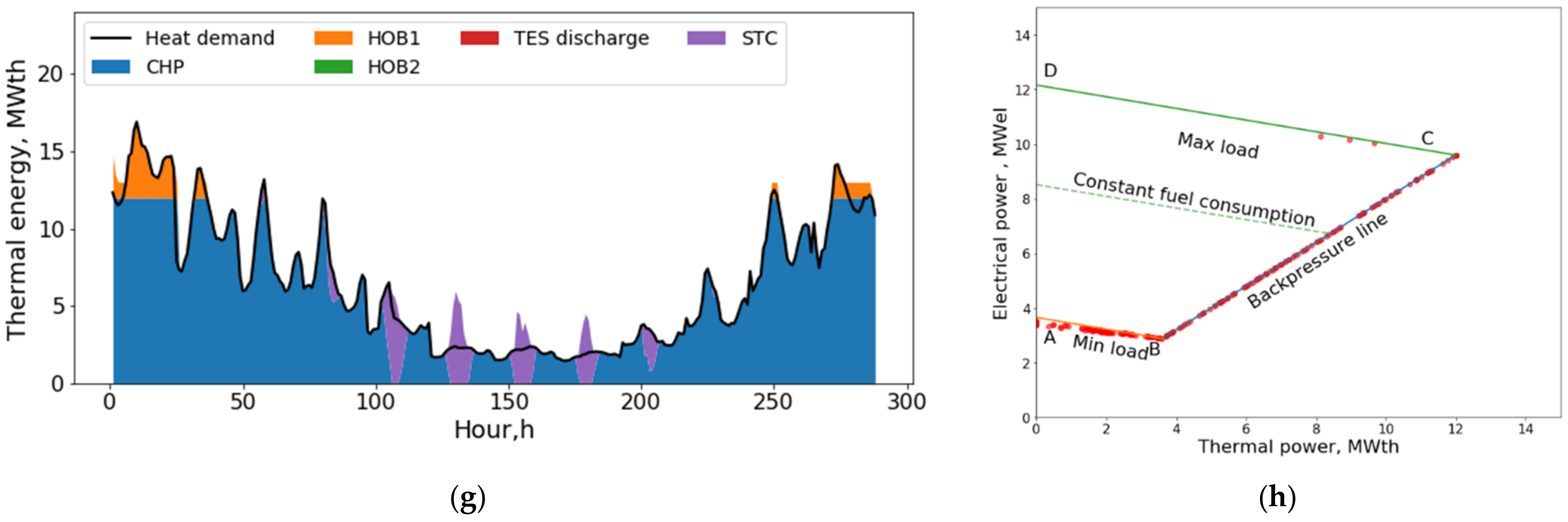
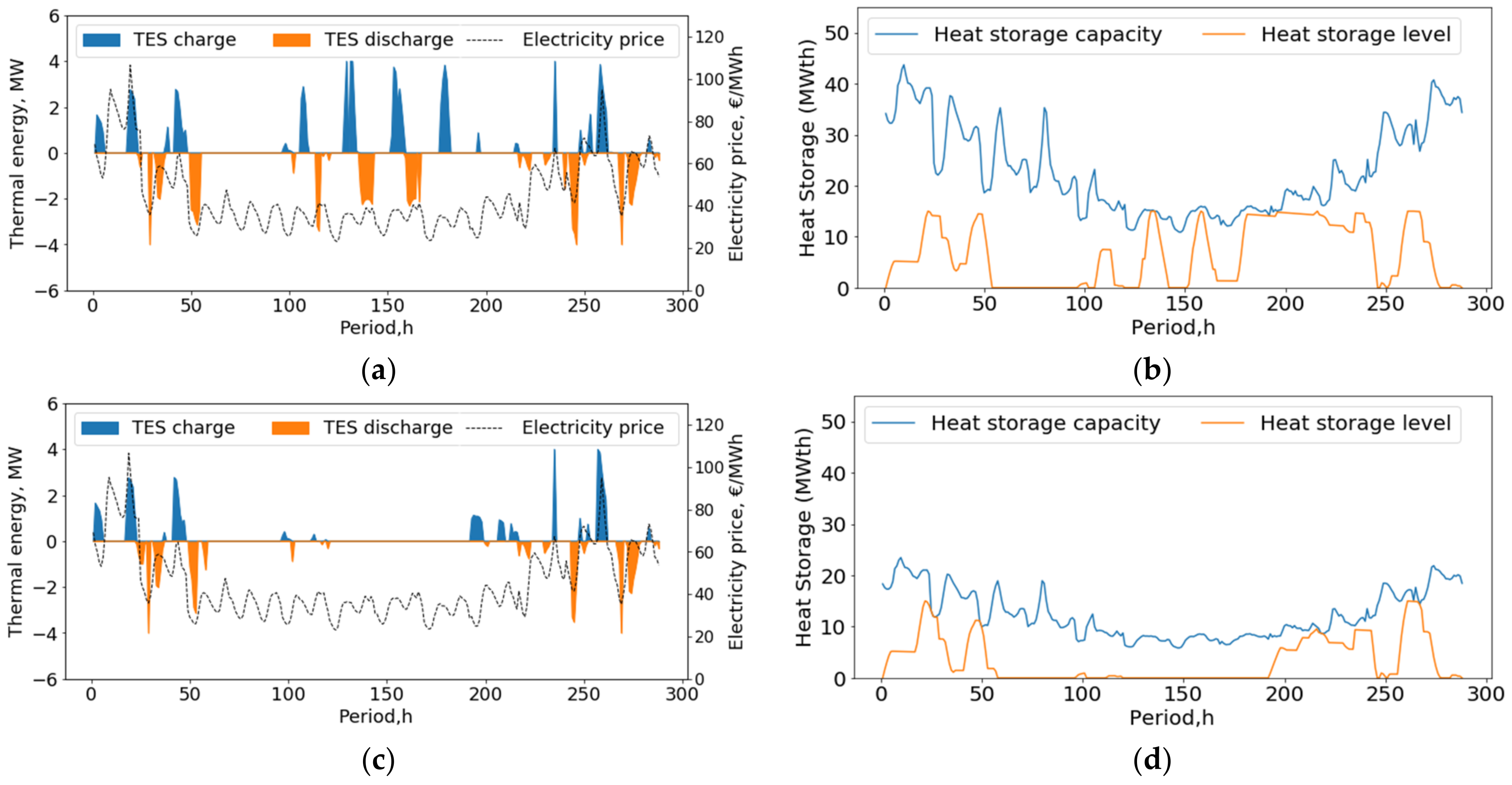
4.3. Hourly Operation Strategy

In this Section, the hourly operation of the optimal systems selected for the 4 scenarios during the typical days are presented and discussed. Figure 12 shows the hourly heat production per system and the hourly operation modes of the CHP on its operational map, over the 12 typical days in a row. It is obvious that integration of TES and STC significantly improve system operation flexibility and efficiency.

First, it can be observed that the TES and the STC systems play an important role in increasing the system flexibility. The system with TES is more flexible as it can achieve peak load shaving and load valley filling, which results in a decrease of the HOB operation [10]. The HOB’s are operated up to 52% less when TES is implemented (Scenarios 2 and 3), as shown in Table 5. In the winter period, the thermal energy supplied by HOB during peak load time in Scenarios 1 is replaced by TES in Scenarios 2 and 3. During the summer period, the daytime heat demand is covered by STC in Scenarios 2 and 4. As expected, the excess heat produced by STC in Scenario 2 is stored in TES and discharged later on when STC cannot meet the demand.

Secondly, the operational flexibility of the CHP unit is also increased by the integration of TES and STC. Figure 12 shows that the CHP operates more on the left-hand part of the A-B line (minimum fuel consumption) in Scenario 2 than in Scenario 1, which helps increasing the electrical power generation for the same fuel consumption and, hence, the same CO₂ emissions.

The detailed performances of the TES system are also shown in Figure 13. TES enables the operation of the system associated with electricity prices, to maximize the profits from selling electricity without affect heat supply safety. Furthermore, TES is more active in the summer period when used in combination with STC. The optimal TES size in Scenario 2 is therefore twice larger than for Scenario 3, see Table 5.

4.4. Sensitive Analysis

The input parameters used in the case study above are prone to uncertainty. To assess the impact of these uncertainties, a sensitivity analysis is carried out for the optimal solution of Scenario 2, for the following key input parameters [37]: heat demand, carbon price, electricity price, fuel price and interest rate.

Figure 14 shows the performance of the optimal solutions in terms of ATC, CO₂ emissions and size of TES and STC, with the variation of the inputs (±20%). It must be noted that each of these results corresponds to an optimal solution computed for the new set of input parameters, and not to the results obtained for the reference optimal solution for other input parameters.

Although they affect the optimal sizes of the TES and STC systems, the influence of economic parameters on the amount of CO₂ emitted in the optimal cases is negligible compared to the influence of the heat demand, see Figure 14a. As far as ATC is concerned (Figure 14b), heat demand and fuel price have a similar impact: ATC increased by 15% when the input parameter increases by 20%. The price of electricity exhibits the opposite trend: the ATC is 12.5% higher when it decreases with 20%, due to the lower revenues from the CHP unit. The price of CO₂ and the interest rate should not be neglected, although they have a lower impact on ATC.

In terms of impact on the systems design in Figure 14c,d, the TES volume is less sensitive to the uncertainties on the inputs than the STC area, which significantly varies with heat demand, fuel price and interest rate. Although this study showed that their combination with TES can result in a profitable reduction of CO₂ emissions, this shows that economic aspects can be a limiting factor in the implementation of STC.

5. Conclusions and Future Work

A framework for the multi-objective optimization of the integration of Solar Thermal Collectors (STC) and Thermal Energy Storage (TES) systems in existing fossil-fuel based heat and power production systems was presented. The proposed method was applied to the representative case of a medium-scale CHP system coupled to a District Heating network. As a comparison, the integration of TES or STC alone was also considered.

The proposed TOPSIS-entropy method has been proved to be efficient to select the optimal design in terms of trade-off between cost and CO₂ reduction. Our results show that, while the addition of TES or STC alone results in limited economic and environmental performances and exhibits a rapid increase of the cost with the targeted CO₂ emission reduction, the optimal combination of TES and STC can lead to a reduction of both the cost and the CO₂ emissions: respectively 3% and 10% in the studied case. For larger CO₂ emissions savings, beyond the optimal trade-off, the additional cost remains limited compared to the other solutions. The integration of TES and STC also significantly improves the system flexibility and efficiency. TES allows for peak load shaving and load valley filling, resulting in up to 52% less operation of peak units. For the optimal design, the total efficiency of the system increases from 87% to 92%. The share of renewable energy reaches 10% when both TES and STC are integrated, compared to 7% with STC alone.

The operational flexibility of the CHP unit itself is also increased by the integration of TES and STC, which helps increasing the electrical power generation.

A sensitivity analysis shows that only the heat demand has a significant impact on the environmental performance, while both the heat demand and the fuel price have a significant influence on the economic performances. Furthermore, the optimal TES volume is less sensitive to the uncertainties on the inputs than the STC surface, that is more impacted by the economic parameters.

In future works, the same methodology could be applied to the integration of more renewable energy sources such as heat pumps and power-to-X based on renewable electricity production. The case of a new CHP unit will also be investigated instead of a retrofit, taking into account the optimal sizing of this unit and the related investment costs. Moreover, the impact of the uncertainties on the input data could be studied using advanced Uncertainty Quantification and Robust Design techniques.

References

1. European Commission. Mapping and Analyses of the Current and Future (2020–2030). Heating/Cooling Fuel Deployment—Executive Summary. Available online: https://energy.ec.europa.eu/mapping-and-analyses-current-and-future-2020-2030-heatingcooling-fuel-deployment-fossilrenewables-1_en (accessed on 6 December 2021).
2. Eurostat. Renewable Energy Statistics. Available online: https://ec.europa.eu/eurostat/statistics-explained/index.php?title=Renewable_energy_statistics (accessed on 6 December 2021).
3. International Renewable Energy Agency. Renewable Energy in District Heating and Cooling. Available online: https://www.irena.org/publications/2017/Mar/Renewable-energy-in-district-heating-and-cooling (accessed on 6 December 2021).
4. Danish Energy Agency. Technology Data: Generation of Electricity and District Heating. Available online: https://ens.dk/sites/ens.dk/files/Analyser/technology_data_catalogue_for_el_and_dh.pdf (accessed on 6 December 2021).
5. Verkis Svartsengi. Power Plant. Available online: https://www.verkis.com/projects/energy-production/geothermal-energy/nr/936 (accessed on 6 December 2021).
6. International Energy Agency (IEA). Large Biomass CHP Plant in Stockholm, Sweden. Available online: https://www.ieabioenergy.com/wp-content/uploads/2018/02/8-LargeCHP-Va%CC%88rtaverket_SE_Final.pdf (accessed on 6 December 2021).
7. Lund, H.; Østergaard, P.A.; Connolly, D.; Ridjan, I.; Mathiesen, B.V.; Hvelplund, F.; Thellufsen, J.Z.; Sorknsæs, P. Energy Storage and Smart Energy Systems. Int. J. Sustain. Energy Plan. Manag. 2016, 11, 3–14. [Google Scholar] [CrossRef]
8. Lund, H.; Werner, S.; Wiltshire, R.; Svendsen, S.; Thorsen, J.E.; Hvelplund, F.; Mathiesen, B.V. 4th Generation District Heating (4GDH). Integrating Smart Thermal Grids into Future Sustainable Energy Systems. Energy 2014, 68, 1–11. [Google Scholar] [CrossRef]
9. Cabeza, L.F.; Miró, L.; Oró, E.; De Gracia, A.; Martin, V.; Krönauer, A.; Rathgeber, C.; Farid, M.M.; Paksoy, H.O.; Martínez, M.; et al. CO2 Mitigation Accounting for Thermal Energy Storage (TES) Case Studies. Appl. Energy 2015, 155, 365–377. [Google Scholar] [CrossRef] [Green Version]
10. Benalcazar, P. Optimal Sizing of Thermal Energy Storage Systems for CHP Plants Considering Specific Investment Costs: A Case Study. Energy 2021, 234, 121323. [Google Scholar] [CrossRef]
11. Mugnini, A.; Comodi, G.; Salvi, D.; Arteconi, A. Energy Flexible CHP-DHN Systems: Unlocking the Flexibility in a Real Plant. Energy Convers. Manag. X 2021, 12, 100110. [Google Scholar] [CrossRef]
12. Lai, F.; Wang, S.; Liu, M.; Yan, J. Operation Optimization on the Large-Scale CHP Station Composed of Multiple CHP Units and a Thermocline Heat Storage Tank. Energy Convers. Manag. 2020, 211, 112767. [Google Scholar] [CrossRef]
13. Savic, D. Single-Objective vs. Multiobjective Optimisation for Integrated Decision Support. In Proceedings of the First Biennial Meeting of the International Environmental Modelling and Software Society, Lugano, Switzerland, 24–27 June 2002; pp. 7–12. [Google Scholar]
14. Ren, H.; Zhou, W.; Nakagami, K.; Gao, W.; Wu, Q. Multi-Objective Optimization for the Operation of Distributed Energy Systems Considering Economic and Environmental Aspects. Appl. Energy 2010, 87, 3642–3651. [Google Scholar] [CrossRef]
15. Fazlollahi, S.; Becker, G.; Ashouri, A.; Maréchal, F. Multi-Objective, Multi-Period Optimization of District Energy Systems: IV—A Case Study. Energy 2015, 84, 365–381. [Google Scholar] [CrossRef]
16. Luo, Z.; Yang, S.; Xie, N.; Xie, W.; Liu, J.; Souley Agbodjan, Y.; Liu, Z. Multi-Objective Capacity Optimization of a Distributed Energy System Considering Economy, Environment and Energy. Energy Convers. Manag. 2019, 200, 112081. [Google Scholar] [CrossRef]
17. Karmellos, M.; Mavrotas, G. Multi-Objective Optimization and Comparison Framework for the Design of Distributed Energy Systems. Energy Convers. Manag. 2019, 180, 473–495. [Google Scholar] [CrossRef]
18. Franco, A.; Versace, M. Multi-Objective Optimization for the Maximization of the Operating Share of Cogeneration System in District Heating Network. Energy Convers. Manag. 2017, 139, 33–44. [Google Scholar] [CrossRef]
19. Wirtz, M.; Hahn, M.; Schreiber, T.; Müller, D. Design Optimization of Multi-Energy Systems Using Mixed-Integer Linear Programming: Which Model Complexity and Level of Detail Is Sufficient? Energy Convers. Manag. 2021, 240, 114249. [Google Scholar] [CrossRef]
20. Wu, Q.; Ren, H.; Gao, W.; Ren, J. Multi-Objective Optimization of a Distributed Energy Network Integrated with Heating Interchange. Energy 2016, 109, 353–364. [Google Scholar] [CrossRef]
21. Verbruggen, A.; Dewallef, P.; Quoilin, S.; Wiggin, M. Unveiling the Mystery of Combined Heat & Power (Cogeneration). Energy 2013, 61, 575–582. [Google Scholar] [CrossRef]
22. Mollenhauer, E.; Christidis, A.; Tsatsaronis, G. Evaluation of an Energy- and Exergy-Based Generic Modeling Approach of Combined Heat and Power Plants. Int. J. Energy Environ. Eng. 2016, 7, 167–176. [Google Scholar] [CrossRef] [Green Version]
23. Wang, H.; Yin, W.; Abdollahi, E.; Lahdelma, R.; Jiao, W. Modelling and Optimization of CHP Based District Heating System with Renewable Energy Production and Energy Storage. Appl. Energy 2015, 159, 401–421. [Google Scholar] [CrossRef]
24. Sveinbjörnsson, D.; Jensen, L.L.; Trier, D.; Bava, F.; Hassine, I.B.; Jobard, X. Fifth Generation, Low Temperature, High Exergy District Heating and Cooling Networks: D2.3 Large Storage Systems for DHC Networks. Available online: https://ec.europa.eu/research/participants/documents/downloadPublic?documentIds=080166e5c2089739&appId=PPGMS (accessed on 6 December 2021).
25. Schmidt, T.; Miedaner, O. Solar District Heating Guidelines. Available online: https://www.solarthermalworld.org/sites/default/files/story/2015-04-03/sdh-wp3-d31-d32_august2012_0.pdf (accessed on 6 December 2021).
26. Chen, P. Effects of the Entropy Weight on TOPSIS. Expert Syst. Appl. 2021, 168, 114186. [Google Scholar] [CrossRef]
27. Li, X.; Wang, K.; Liuz, L.; Xin, J.; Yang, H.; Gao, C. Application of the Entropy Weight and TOPSIS Method in Safety Evaluation of Coal Mines. Procedia Eng. 2011, 26, 2085–2091. [Google Scholar] [CrossRef] [Green Version]
28. Ding, L.; Shao, Z.; Zhang, H.; Xu, C.; Wu, D. A Comprehensive Evaluation of Urban Sustainable Development in China Based on the TOPSIS-Entropy Method. Sustainability 2016, 8, 746. [Google Scholar] [CrossRef] [Green Version]
29. Epexspot. EPEX SPOT 2021. Available online: https://www.epexspot.com/en (accessed on 6 December 2021).
30. European Commission. JRC Photovoltaic Geographical Information System (PVGIS)—Commission. Available online: https://re.jrc.ec.europa.eu/pvg_tools/en/#MR (accessed on 6 December 2021).
31. Benalcazar, P. Sizing and Optimizing the Operation of Thermal Energy Storage Units in Combined Heat and Power Plants: An Integrated Modeling Approach. Energy Convers. Manag. 2021, 242, 114255. [Google Scholar] [CrossRef]
32. Morvaj, B.; Evins, R.; Carmeliet, J. Optimising Urban Energy Systems: Simultaneous System Sizing, Operation and District Heating Network Layout. Energy 2016, 116, 619–636. [Google Scholar] [CrossRef]
33. Fazlollahi, S.; Becker, G.; Maréchal, F. Multi-Objectives, Multi-Period Optimization of District Energy Systems: II-Daily Thermal Storage. Comput. Chem. Eng. 2014, 71, 648–662. [Google Scholar] [CrossRef]
34. Limpens, G.; Moret, S.; Jeanmart, H.; Maréchal, F. EnergyScope TD: A Novel Open-Source Model for Regional Energy Systems. Appl. Energy 2019, 255, 113729. [Google Scholar] [CrossRef]
35. Quaschning, V. Understanding Renewable Energy Systems; Routledge: Abingdon, UK, 2005; Volume 67, ISBN 9781844071289. [Google Scholar]
36. Worldbank. Carbon Pricing Dashboard, Up-to-Date Overview of Carbon Pricing Initiatives. Available online: https://carbonpricingdashboard.worldbank.org/map_data (accessed on 6 December 2021).
37. Akbari, K.; Nasiri, M.M.; Jolai, F.; Ghaderi, S.F. Optimal Investment and Unit Sizing of Distributed Energy Systems under Uncertainty: A Robust Optimization Approach. Energy Build. 2014, 85, 275–286. [Google Scholar] [CrossRef]
Figure 1. Optimization Framework of hybrid energy system.
Energies 15 01942 g001
Figure 2. Schematic of Hybrid energy system.
Energies 15 01942 g002
Figure 3. Cogeneration of Power and heat extraction for EC based CHP plant.
Energies 15 01942 g003
Figure 4. Normalized efficiency for HOB, according to [19].
Energies 15 01942 g004
Figure 5. Investment costs for TES systems: (a) Specific investment cost according to [24]; (b) Cumulative investment cost.
Energies 15 01942 g005
Figure 6. Investment costs for STC: (a) Specific investment cost according to [25]; (b) Cumulative investment cost.
Energies 15 01942 g006
Figure 7. Flowchart of Decision-making process.
Energies 15 01942 g007
Figure 8. Heat Load in: (a) one year; (b) monthly typical days.
Energies 15 01942 g008
Figure 9. Electricity price in: (a) one year; (b) monthly typical days [29].
Energies 15 01942 g009
Figure 10. Hourly variation of ambient temperature and solar irradiance over the year [30].
Energies 15 01942 g010
Figure 11. Relative Pareto frontiers for Scenarios relative to Scenario 1.
Energies 15 01942 g011
Figure 12. Hourly heat production for all Scenarios over the 12 typical days in a row: (a) Hourly Heat production of Scenario 1; (b) CHP operation field of Scenario 1; (c) Hourly Heat production of Scenario 2; (d) CHP operation field of Scenario 2; (e) Hourly Heat production of Scenario 3; (f) CHP operation field of Scenario 3; (g) Hourly Heat production of Scenario 4; (h) CHP operation field of Scenario 4.
Energies 15 01942 g012aEnergies 15 01942 g012b
Figure 13. Charging or discharging load and heat storage levels of TES over the 12 typical days in a row: (a) TES charging and discharging load of Scenario 2; (b) TES heat storage levels of Scenario 2; (c) TES charging and discharging load of Scenario 3; (d) TES heat storage levels of Scenario 3.
Energies 15 01942 g013
Figure 14. Sensitivity of the main results to the variation of key input parameters: (a) CO2 generation; (b) ATC; (c) TES volume; (d) STC area.
Energies 15 01942 g014