A Technique of Hydrocarbon Potential Evaluation in Low Resistivity Gas-Saturated Mudstone Horizons in Miocene Deposits, South Poland

Abstract

The petrophysical properties of Miocene mudstones and gas bearing-heteroliths were the main scope of the work performed in one of the multihorizon gas fields in the Polish Carpathian Foredeep. Ten boreholes were the subject of petrophysical interpretation. The analyzed interval covered seven gas-bearing Miocene horizons belonging to Sarmatian and Badenian deposits. The water saturation in shaly sand and mudstone intervals was calculated using the Montaron connectivity theory approach and was compared with Simandoux water saturation. Additionally, the Kohonen neural network was used for qualitative interpretation of four PSUs (petrophysically similar units), which represent the deposits of comparable petrophysical parameters. This approach allowed us to identify the sediment group with the highest probability of hydrocarbon saturation. Then, the spatial distribution of PSUs and reservoir parameters was carried out in Petrel. The resolution of the model was selected to reflect the variability of log-derived parameters. The reconstruction of the spatial distribution of shale volume, porosity, and permeability was performed with standard parametric modeling procedures using the Gaussian random function simulation stochastic algorithm, while PSU distribution and hydrocarbon saturation (SH) required a separate approach. The distribution into PSU groups was carried out by facies classification. Predefined ranges of clay volume, effective porosity, and permeability were used as discriminators to achieve spatial distribution of the PSU groups. The spatial distribution of hydrocarbon saturation was performed by creating the meta-attribute of this parameter and then reducing the derived pseudo-saturation model to physical values. Results included the creation of maps of hydrocarbon saturation that show the preferable areas with the highest hydrocarbon saturation for each gas horizon.

1. Introduction

Research on hydrocarbons in Miocene sediments of the Carpathian Foredeep conducted in recent years has led to the discovery of many gas horizons located in thin-layer heteroliths, mudstones, and sandstones. Many geophysical and geological research has been performed to recognize the possibilities of hydrocarbon accumulation in Miocene sediments [1,2,3,4,5,6,7]. The main influence on the formation of gas accumulations was the structural and facies factors, which define the horizons lithological boundaries [1]. There are three main sedimentary complexes in the study area: deltaic deposits, submarine fan sediments and fine-rhytmic turbidyte sediments of basin plain. The lowest part of the upper Baden-Sarmatian is dominated by heterolithic deposits formed in the environment of the basin plain. They consist of claystones and siltstones covered with thin layers of fine and medium-grained sandstones, the thickness of these sediments can be up to about 200 m. Higher in the profile the turbidite sediments of submarine fans can be observed. They are spread under the Carpathian thrust and along its present border. The thickness of these sediments can reach several meters and are the result of sedimentation within the distribution channels of the upper fan. Finer turbidite sediments are associated with sedimentation along the riverbed shafts. These sediments are about 300 m thick. Towards the top of the profile, the series of submarine fans turbidite deposits are gradually replaced by deltaic deposits of rather constant thickness. Deltaic deposits are characterized by a clay-sandy lithology and generally high collateral continuity. The sandstones of deltaic sediments, especially occurring in thin-bed heterolithic and mudstone lithofacies, are characterized by low textural and mineral maturity. The sandstones grain skeleton is composed of a very fine to medium-grained fraction [1,2,3].

The interesting is that despite there is sandstones complex with thickness of even 250 m, formed as submarine fans sediments with the excellent porosity and permeability, the existing hydrocarbon horizons mainly occurs in sandstones up to 50 m of thickness. It is probably due to dispersion of hydrocarbons in layers of large thickness [1]. There are not enough sealing units to prevent migration of hydrocarbons. The morphology of Precambrian basement had the main impact for developing of the deepest located gas accumulations mainly within fine-rhytmic turbidyte heteroliths being the subject of the interpretation in the presented work. The detail recognition and reconstruction of sedimentary environment and building a proper structural model is a main task to predict the stratigraphic traps which constitute favorable areas for hydrocarbon accumulations [1]. Seismostratigraphic works performed in the area of Wielkie Oczy—Graben and Markowce-Lubliniec elevation allowed to subdivide the Machow formation into seven genetic sequences composed mostly of deltaic deposits. The work allowed to detect the upplaping pinchouts that constitute structural-stratigraphic traps for gas generated in front-prodelta heteroliths [6]. In the area seismic-scale deltaic clinoforms can be observed on the south, these forms developed a shelf-to-basin floor relief of over 300 m [3].

However, the detection of hydrocarbon-saturated intervals still remains the greatest challenge. Resistivity logs measured in shaly-sand intervals show low values, as the occurrence of clay minerals constitute additional conductive components apart from water present in the rock. Shaly-sand formations are usually related to the high content of capillary water occupying the matrix micropores. Due to the high volume of clay minerals, there are many intervals with ambiguous saturation characteristics. Thus, a novel approach is required to detect low-resistivity gas-saturated zones. Mudstones are “non-Archie rock”, where the saturation exponent (n) is not a constant, but its values change throughout the reservoir. It is expected that the saturation exponent in mudstones is low, as these sediments are likely to be wet. Thus, the Montaron equation [8] was adopted to calculate water saturation, where rock wettability is expressed through the water connectivity index (WCI). Additionally, the artificial neural network approach was used to identify the unit of the best gas accumulation properties and particularly to separate gas-saturated and water-saturated intervals. The process of water saturation estimation was supported by the modified qualitative Passey’s [9] and Bowman’s [10] methods primary dedicated the calculation of TOC content. A successful result of the analyses carried out in the profiles of the boreholes consequently raises the issue of the spatial distribution of these reservoir parameters. Thus, the authors attempt to reliably recreate the spatial continuity of the reservoir’s parameters obtained from well logs through the use of geostatistical analyzes, multiple linear regression and neural network techniques in the face of the availability of seismic data. As seismic data are available, the results were integrated into the spatial seismic response through the use of supervised neural network methods. Finally, an attempt was made to identify the areas preferable for planning future wells with high gas accumulation potential.

2. Materials and Methods

2.1. Study Area

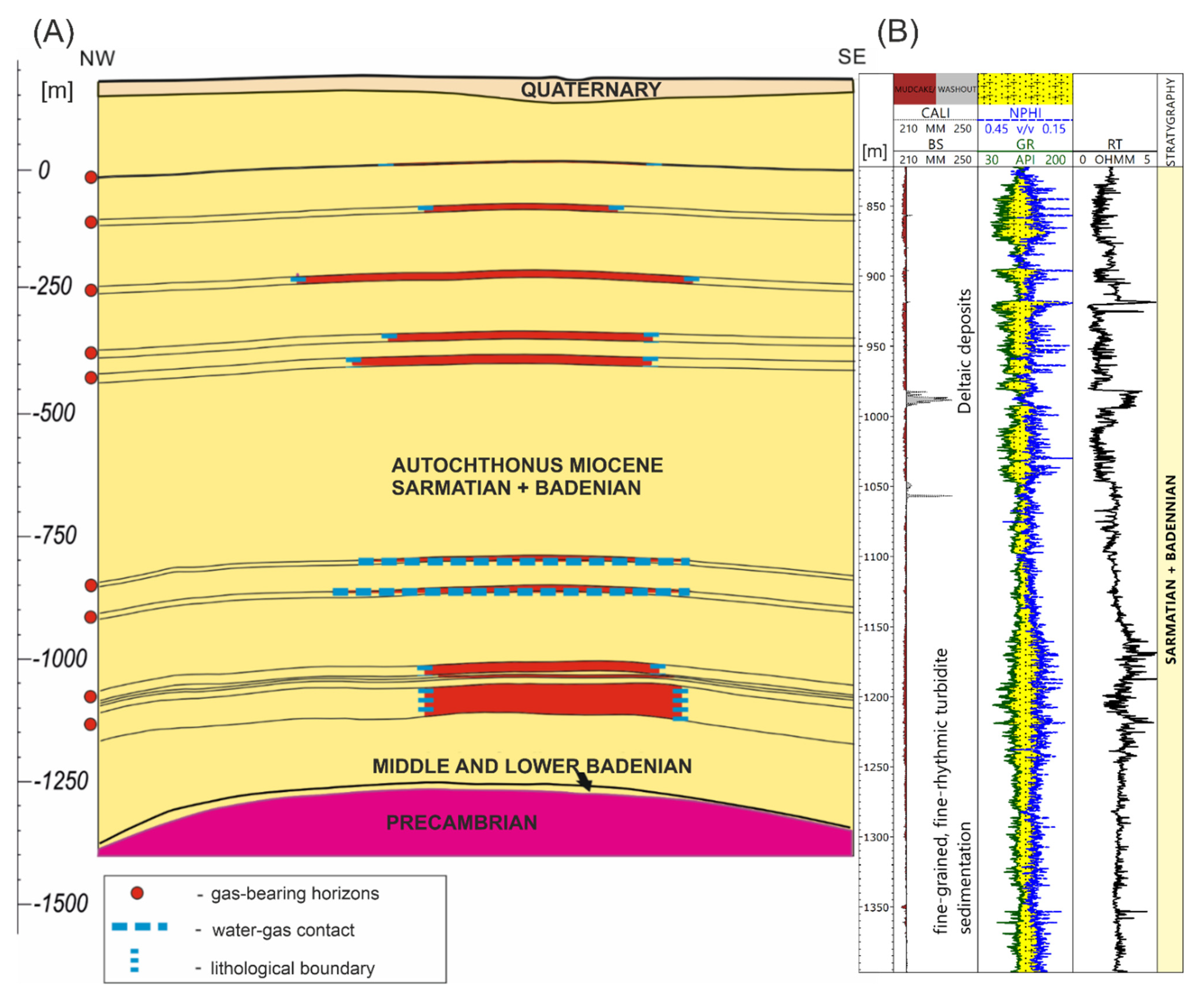
The location of the study is an area of multihorizon gas deposits typical of Miocene formations (Figure 1A). The analyzed area is in the central part of the Carpathian Foredeep, a short distance from the edge of the Carpathian overthrust, and is characterized by an uncomplicated geological structure, both in terms of stratigraphy and tectonics, which consists of three main complexes: (1) Precambrian basement with a strongly eroded morphological surface; (2) autochthonous Miocene sediments subdivided into Sarmatian and Badenian; and (3) Quaternary cover. Eroded Precambrian basement, consisting of quartzite sandstone and shales, is unconformably overlain by Badenian and Sarmatian sediments where many gas-bearing horizons were discovered. The Badenian formation consists of clays, marly clays, marls with thin laminas of mudstones, sandstones, and anhydrites. The Upper Badenian deposits are represented in the entire area by clay and clay–calcareous shales, sometimes interbedded with sandstone. The Sarmatian sediments consist of sandstone, mudstone, and claystone layers of similar thickness. The Sarmatian claystones are represented by gray, dark gray, and marly clayey shales with inserts and interlayers of light gray and gray fine-grained calcareous sandstones. The upper part of the Lower Sarmatian is associated with the presence of silty sands and claystones, while more sandstone layers are observed at greater depths. The Quaternary cover, up to 30 m, consists of clay, silt, sand, and gravel, from which gas exhalations from the underlying unsealed deposits or uninsulated boreholes were observed. This is related to the nature of hydrocarbon migration processes resulting from pressure differences, capillary forces, diffusion phenomena, etc. [11,12,13]. Gas-bearing horizons associated with the Lower Sarmatian are formed as sandstone and mudstone layers with good reservoir properties, which have an anticlinal structure. The series of sandstone and mudstone were also found to dip at small angles (1–2 degrees). Their average thickness is approximately 11 m (from 1 to 25 m effective thickness) with an average gas saturation of 63% (gas saturation from 52 to 83%). The average porosity and permeability of the gas horizons of this area are, respectively, 7.4% and 26 mD, with the maximum recorded values of these parameters equal to 30% and 2700 mD. Reservoir properties decrease due to compaction and the increase in calcite in the lithologic composition. The interbeds of claystones constitute an impervious barrier to the migration of gas, which is characterized by high methane content (not less than 95.77% CH₄) [14]. The individual gas accumulation is determined by the water–gas contact or lithological barrier related to changes in the sedimentary depositional environment. There are also gas accumulations related to fractures and cracks in the upper part of the Precambrian deposits, isolated by impervious anhydrite layers, but these gas occurrences are not a subject of this study.

2.2. Input Data

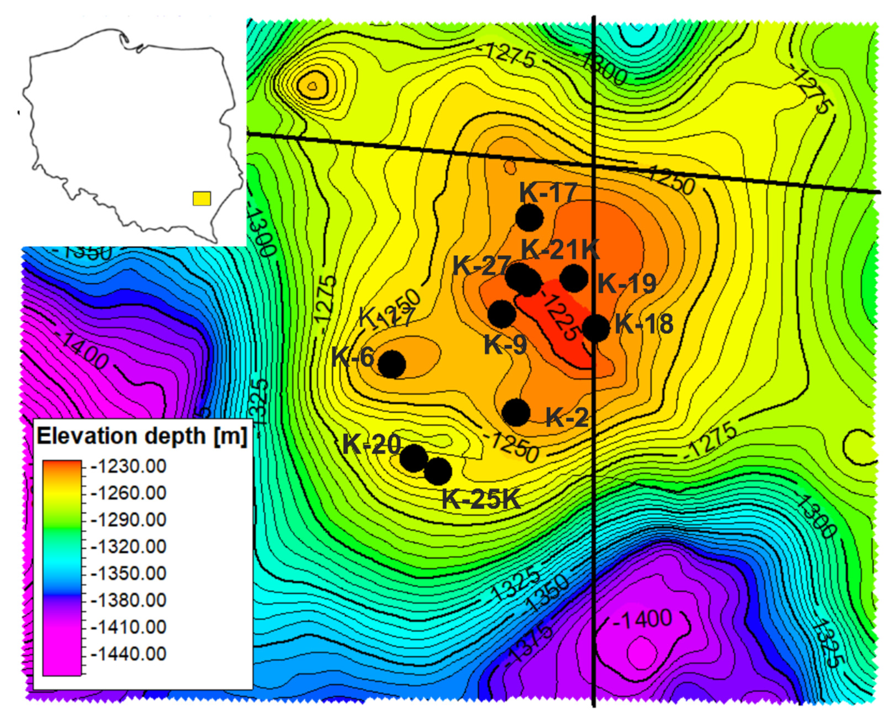
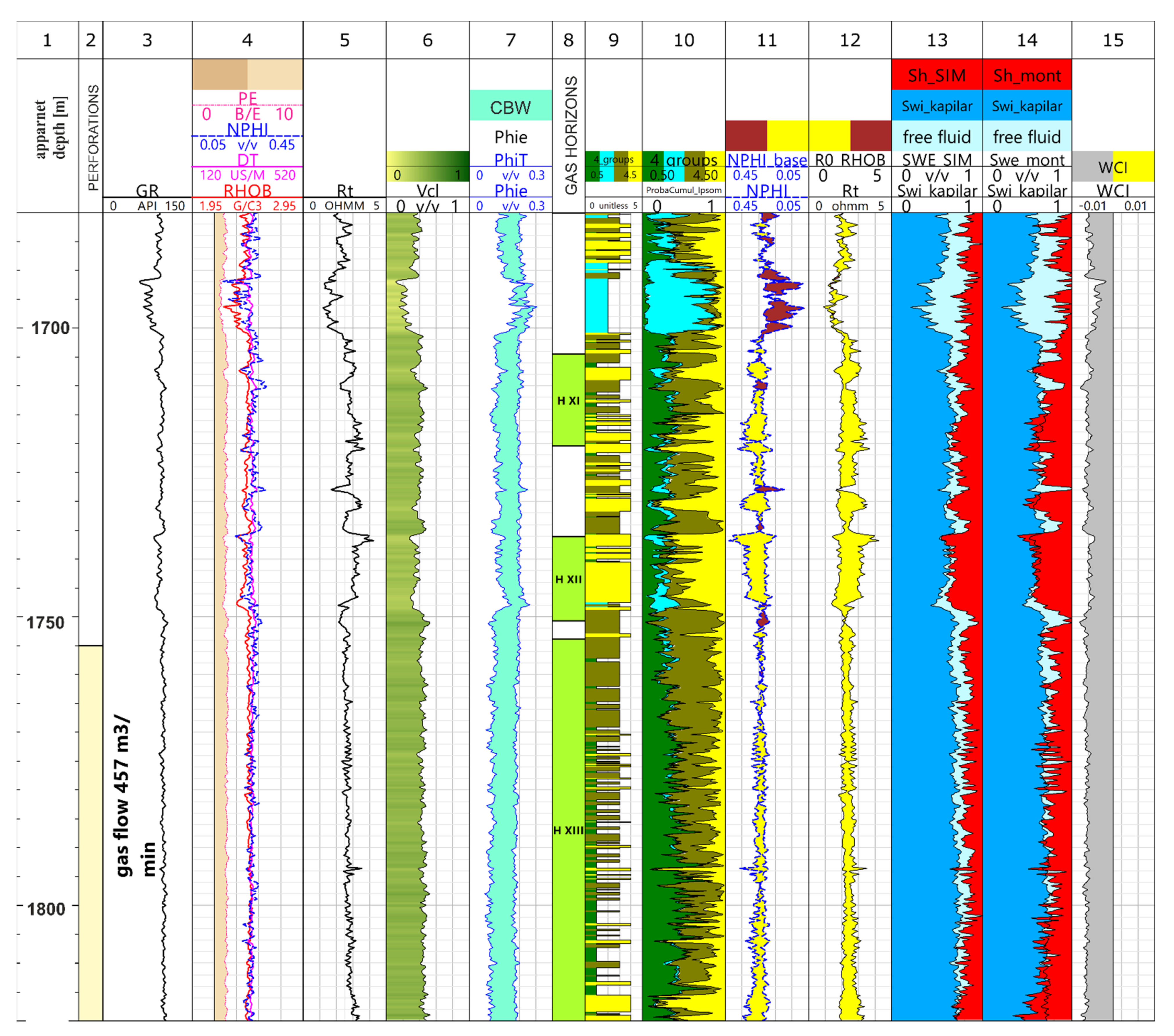
The petrophysical interpretation was carried out using data from 10 boreholes within several hundred meters of Miocene sediments covering 7 gas-bearing horizons. The gas deposit formed as anticline with the location of the wellbores is presented in Figure 2.

K-6, and K-9 wells, drilled in the 1970s and 1980s, represent a much lower technical level than the wells drilled in recent years (2011–2015). Thus, the analyzed wells differ significantly in quality, technical conditions, and available well log data. The standard dataset from the 1970s and 1980s included the following well logs: gamma ray (GR), neutron porosity (NPHI), resistivity logs (EN64, EN16, EL18), diameter (CALI), and spontaneous potential (PS).

The first stage of the work was to collect the available laboratory and stratigraphic data, core descriptions, reservoir test information, and well logs available from individual boreholes. For wells K-17, K-18, K-19, K-20, and K-21K, the following laboratory measurements were performed: porosity measurement by MIP (mercury injection porosimetry) method, permeability measurements, NMR, XRD, and measurement of the Archie parameter (cementation exponent (m)). These boreholes were used to establish the relationships between well logs and laboratory data. They were the basis for the interpretation of older wells characterized by inferior technical conditions and limited sets of well logs. Laboratory analyses carried out on the cores were the basis for the calibration of effective porosity (correlation between laboratory-measured bulk density and effective porosity), the definition of the relationship between porosity (PHIE) and permeability (K), and calculation of the irreducible water content (Swi_Kapilar) based on NMR data. Moreover, the XRD data enabled us to calibrate the calculated clay volume. Datasets of new boreholes additionally include the following logs: PE (photoelectric factor), DT (compressional slowness), bulk density (RHOB), and medium (ILM) and deep (ILD) induction resistivity logs.

Table 1. Well log data available for the interpreted wells.

Well Name	Available Well Logs	Laboratory Core Measurements
K-2	CALI, GR, SP, NPHI, EL18, EN16, EN64	PHIE, Perm., RHOB
K-6	CALI, GR, SP, NPHI, EL18, EN16, EN64	PHIE, Perm., RHOB
K-9	CALI, GR, SP, NPHI, EL18, EN16, EN64
K-17	CALI, GR, PE, NPHI, DT, RHOB, PE, ILM, ILD	PHIE, NMR, XRD
K-18	CALI, GR, PE, NPHI, DT, RHOB, PE, ILM, ILD	PHIE, NMR, XRD
K-19	CALI, GR, PE, NPHI, DT, RHOB, PE, ILM, ILD	PHIE, NMR, XRD
K-20	CALI, GR, PE, NPHI, DT, RHOB, PE, ILM, ILD	PHIE, NMR, XRD
K-21K	CALI, GR, PE, NPHI, DT, RHOB, PE, ILM, ILD, URAN, POTAS, THOR
K-25K	CALI, GR, PE, NPHI, DT, RHOB, PE, ILM, ILD, URAN, URAN, THOR
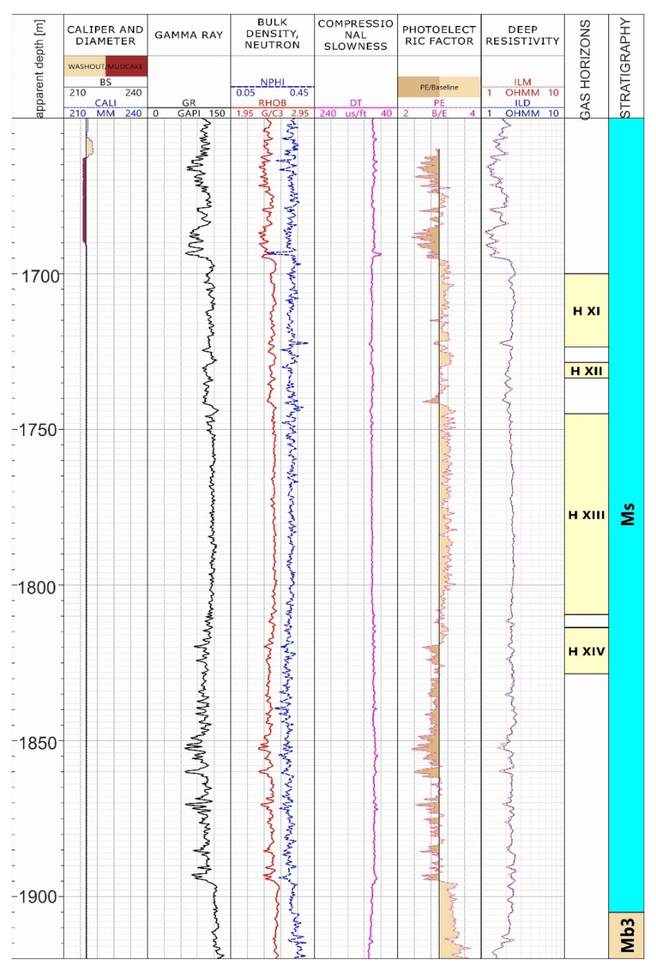
K-27	CALI, GR, PE, NPHI, DT, RHOB, PE, ILM, ILD

contains the input data used in the interpretation, and Figure 3 is a graphical presentation of the input data from the K-17 well. In boreholesK-25K and K-27, there were also available measurements of potassium (POTA), thorium (THOR), and uranium (URAN) concentration.

2.3. Evaluation of Reservoir Parameters from Well Logs (Vcl, Phie, Swi)

The shaly-sand reservoir, due to high clay volume content and rather low porosity, belongs to unconventional gas accumulation, and the applied methodology of water saturation differs from the classical methods used in the analysis of conventional deposits. The approach to calculate other reservoir parameters such as clay volume (Vcl), effective porosity (Phie), and irreducible water saturation (capillary-bound water) (Swi_kapilar) was based on well logging and laboratory measurements from cored intervals together with the results of well tests. In order to evaluate the key reservoir parameters, a simple petrophysical model was built. The results of X-ray diffraction laboratory measurement and crossplots of Potassium and Thorium concentration indicate show that the dominant clay minerals are: illite and montmorillonite, while rock matrix consists of quartz with admixtures of K-Feldspar, Plagioclase, Calcite and Dolomite.

clay volume + matrix + porosity

The best calibration of the volumetric content of clay minerals with the results of laboratory measurements of total clay mineral content using the X-ray diffraction method was obtained using the Stieber model for Miocene and Pliocene deposits in the form of Equation (1).

$$\mathrm{Vcl}=\frac{\mathrm{GRindex}}{3-2\times \mathrm{GRindex} }$$

(1)

where

$$\mathrm{GRindex} =\frac{\mathrm{GR}-\mathrm{GRmatrix}}{\mathrm{GRcl}-\mathrm{GRmatrix}},$$

and GRcl is the gamma ray for clay, and GRmatrix is the gamma ray value for the sandstones.

The calculations assumed values of GR, namely, 30–40 API for sandstones and 120–160 API for claystones. These values were determined during optimization procedures. Moreover, the correlation between GR and laboratory XRD measurements of total clay mineral content was also performed. The following relationship was obtained Equation (2):

Vcl = 0.455 × GR − 29.95

(2)

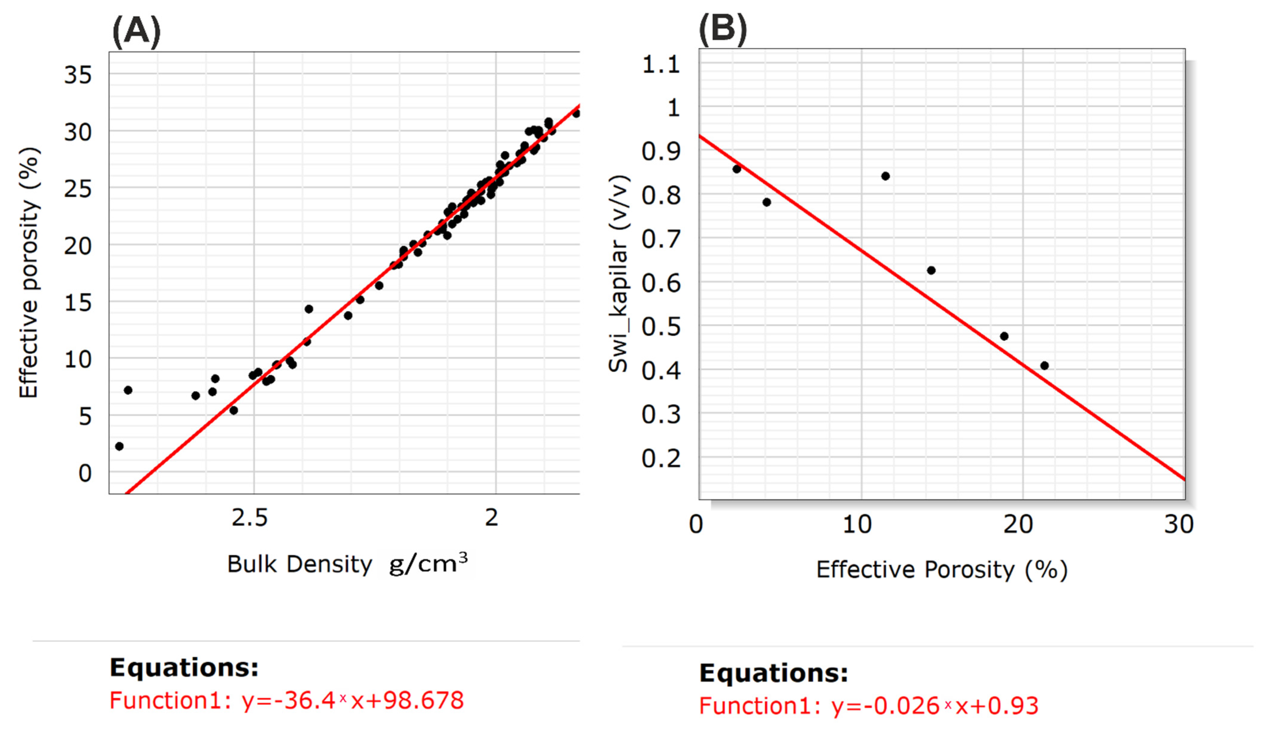
This dependence was used to estimate the clay volume in individual wells. The effective porosity values (Phie) were calculated using two approaches from neutron density log crossplots and using laboratory-measured effective porosity (PHIE) and bulk density (RHOB) (Figure 4A). The neutron porosity of clay, NPHI_Vcl = 0.4, and bulk density of clay, RHOB_Vcl = 2.45, were empirically derived. The total porosity was estimated on the assumption that the clay porosity was Phie_cl = 0.2. The assumption of clay porosity was based on the relationship between total clay volume obtained from the X-ray diffraction analysis technique (XRD) and clay-bound water saturation from NMR data.

PhiT = Phie + Vcl × Phi_cl

(3)

Calculation of capillary water content (Swi_Kapilar), water bound in small pores in the matrix, was also performed with the use of NMR laboratory measurements. A trend line was determined between capillary water saturation and effective porosity (NMR) (Figure 4B), and based on this relationship, Swi_Kapilar was calculated. Each equation based on the use of well logs required the assumptions of certain coefficients; some of these parameters are often unknown and challenging to calculate, especially in shaly-sand or mudstone formations. Errors during the stage of calculating the effective porosity undoubtedly have a large effect on errors in gas resource estimation. More particularly, if the reservoir has moderate to low effective porosity, then much attention should be given to the precise estimation of this parameter.

2.4. Qualitative and Quantitative Methods of Identifying Perspective Gas-Saturated Zones

The most important step during petrophysical interpretation is detection of perspective gas-saturated intervals (qualitative methods), which is followed by calculation of water saturation. Interpretation of gas accumulation present in mudstones is difficult due to high clay volume, which, due to high conductivity, lowers the values of recorded resistivities. Clays, similar to water, are additional conductive media in the formation. This usually leads to underestimation of gas resources.

According to Archie’s assumption [15], the presence of hydrocarbons in rock is related to the difference between the resistivity of the unflushed zone (Rt) and the water-saturated zone (R0). Then, knowing the values of the saturation coefficient (n), one can determine the values of Sw. However, when the interpretation of water saturation is carried out through a formation with a thickness of several hundred meters, consisting of thin layers of sandstone, mudstones, and claystones, proper determination of the saturation exponent (n) is very difficult. The values of this parameter are closely related to the irreducible water content, size of the pores, and wettability of the rock. The resistivity of the water-saturated zone (R0) can be calculated based on formation water resistivity (R_w) and Archie parameters: cementation exponent (m), and saturation exponent (n). Calculation of R_w values requires information about the temperature in the borehole and the salinity. While the temperature in the borehole can be determined based on the results of temperature logs performed in some boreholes in evaluated gas fields or calculated based on temperature gradients for a given area, the salinity/mineralization of water is often unknown. Even the laboratory-measured mineralization of a water sample collected from the evaluated borehole does not guarantee that this sample is not a mixture of mud filtrate and formation water. A more reliable method to determine R0 could be based on well logs measured in situ that reflect the reservoir conditions. The analyzed interval consists of gas-saturated sandstones/mudstones and water-saturated sandstones/mudstones. On the crossplot of bulk density (RHOB) and formation resistivity (Rt), the separation between the gas-saturated zone and the water-saturated zone is clearly visible, especially in the intervals with low clay volume. Thus, the resistivity of the water-saturated zone R0 can be calculated with the use of exponential Equation (4):

$$\mathrm{R}0=\mathrm{a}\times {\mathrm{RHOB}}^{\mathrm{b}}$$

(4)

where a and b are empirically derived constants; for this study, a = 0.0008 and b = 8.8554.

If the bulk density log is not available, the neutron porosity log can also be used.

The presence of hydrocarbons can be defined by the RI (resistivity index) Equation (5):

$$\mathrm{RI}=\frac{\mathrm{Rt}}{\mathrm{R}0}=\frac{\mathrm{Rt}}{\mathrm{a}\times {\mathrm{RHOB}}^{\mathrm{b}}}$$

(5)

Then, the RI obtained can be calibrated with laboratory-measured Sw values, determined, for example, by the Dean–Stark method. During Dean–Stark extraction, a fresh core sample is weighed and subjected to fluid extraction by boiling solvent. Then water is condensed and collected. These laboratory measurements are highly recommended for this type of formation in order to calibrate the water saturation. Unfortunately, there were no laboratory water saturation data available in the evaluated gas field. In this case, the values of Sw were calculated with the use of the generalized connectivity Equation (6) [16,17]:

$$\mathrm{RI}={\left(\frac{1-\mathrm{Sc}}{\mathrm{Sw}-\mathrm{Sc}}\right)}^{\mathsf{\mu }}$$

(6)

where Sc is critical water saturation.

Assuming as a conductive medium: irreducible water bound in clay minerals (CBW), irreducible capillary water held by capillary forces in matrix micropores (KBW) and free water (FFW), and with the assumption that CBW has different resistivity than KBW and free water (FFW), the following equations can be derived [18]:

$$\mathsf{\sigma }={\left[\left(\mathrm{CBW}+\mathrm{KBW}+\mathrm{FFW}\right)\times \mathrm{PhiT}-\mathrm{WCIsh}\right]}^{\frac{1}{\mathsf{\mu }}}$$

(7)

$$\begin{array}{c}{\mathrm{WCI}}_{\mathrm{sh}}\hfill \\ =\left(\mathrm{CBW}+\mathrm{KBW}+\mathrm{FFW}\right)\times \mathrm{PhiT}\hfill \\ -\left[\frac{\mathrm{CBW}\times \mathrm{PhiT}\times {\mathsf{\sigma }}_{\mathrm{cw}}{}^{\frac{1}{\mathsf{\mu }}}+\mathrm{KBW}\times \mathrm{PhiT}\times {\mathsf{\sigma }}_{\mathrm{w}}{}^{\frac{1}{\mathsf{\mu }}}+\mathrm{FFW}\times \mathrm{PhiT}\times {\mathsf{\sigma }}_{\mathrm{w}}{}^{\frac{1}{\mathsf{\mu }}}}{{\mathsf{\sigma }}_{\mathrm{w}}{}^{\frac{1}{\mathsf{\mu }}}}\right]\hfill \end{array}$$

(8)

$$\begin{array}{c}{\mathrm{WCI}}_{\mathrm{sh}}=\left(\mathrm{CBW}+\mathrm{KBW}+\mathrm{FFW}\right)\times \mathrm{PhiT}\hfill \\ \hspace{1em}\hspace{1em}\hspace{1em}\hspace{1em}\hspace{1em}\hspace{1em}\hspace{1em}-\left[\frac{\mathrm{CBW}\times \mathrm{PhiT}\times {\mathsf{\sigma }}_{\mathrm{cw}}{}^{\frac{1}{\mathsf{\mu }}}}{{\mathsf{\sigma }}_{\mathrm{w}}{}^{1/\mathsf{\mu }}}+\frac{\mathrm{KBW}\times \mathrm{PhiT}\times {\mathsf{\sigma }}_{\mathrm{w}}{}^{\frac{1}{\mathsf{\mu }}}}{{\mathsf{\sigma }}_{\mathrm{w}}{}^{1/\mathsf{\mu }}}+\frac{\mathrm{FFW}\times \mathrm{PhiT}\times {\mathsf{\sigma }}_{\mathrm{w}}{}^{\frac{1}{\mathsf{\mu }}}}{{\mathsf{\sigma }}_{\mathrm{w}}{}^{1/\mathsf{\mu }}}\right]\hfill \end{array}$$

Then,

$${ \mathrm{WCI}}_{\mathrm{sh}}=\mathrm{CBW}\times \mathrm{PhiT}\left[1-{(\frac{{\mathsf{\sigma }}_{\mathrm{cw}}}{{\mathsf{\sigma }}_{\mathrm{w}}})}^{1/\mathsf{\mu }}\right]$$

$${\mathrm{WCI}}_{\mathrm{sh}}=\mathrm{CBW}\times \mathrm{PhiT}\left[1-{(\frac{{\mathrm{R}}_{\mathrm{w}}}{{\mathrm{R}}_{\mathrm{cw}}})}^{1/\mathsf{\mu }}\right]$$

$$\mathrm{Sc}=\frac{\mathrm{WCI}}{\mathrm{PhiT}}$$

$$\mathrm{Sc}=-\mathrm{CBW}\times \left[{\left(\frac{{\mathrm{R}}_{\mathrm{w}}}{{\mathrm{R}}_{\mathrm{cw}}}\right)}^{\frac{1}{\mathsf{\mu }}}-1\right]$$

(9)

• WCI—water connectivity index
• CBW—clay-bound water, water bound in clay minerals
• KBW—capillary-bound water, water bound in the micropores of the rock matrix
• FFW—free fluid water, moveable water
• ${\mathsf{\sigma }}_{\mathrm{w}}$—conductivity of free water and KBW
• ${\mathsf{\sigma }}_{\mathrm{cw}}$—conductivity of CBW
• R_w—free fluid water (FFW) and capillary-bound water (KBW) resistivity
• R_cw—clay-bound water resistivity
• μ—conductivity exponent
• Swir = CBW × PhiT and Swi_Kapilar = KBW × Phie

Thus, the final water saturation (Sw) can be calculated as

$$\mathrm{Sw}=\frac{\left(1-\mathrm{Sc}\right)+\sqrt[\mathsf{\mu }]{\mathrm{RI}}\times \mathrm{Sc}}{\sqrt[\mathsf{\mu }]{\mathrm{RI}}}$$

(10)

The values of the conductivity coefficient μ are generally constant, and their range of variation is small (1.6–2).

2.5. Determination of Critical Water Saturation (Sc)

Although RI index can be calculated based on in situ measurement, the estimation of Sc values may require the values of R_w and R_cw. Thus, formation/free water resistivity (R_w) was calculated on the basis of the salinity of the water measured in the laboratory and the temperature measured in the borehole. The (R_w) values decreased with depth. In the interval below 1000 m, the R_w values ranged from 0.02 to 0.058 ohm. Resistivity of clay-bound water was calculated as follows Equation (11):

$${\mathrm{R}}_{\mathrm{cw}}=\frac{\mathrm{CBW}\times \mathrm{PhiT}}{\mathrm{m}}\times \frac{\mathrm{Rvcl}}{\mathrm{a}}$$

(11)

The cementation exponent (m) was calculated based on the relationship between laboratory-measured values of m and measured porosity, performed in well K-17 (12).

m = 0.089 × log (Phie) + 1.952

(12)

However, if there are difficulties in cementation exponent calculation, no measurements of m are performed in the evaluated gas field. The simple equation proposed by Peeters &Holmes [19] can be used to calculate conductivity (C_cw) and resistivity (R_cw) of clay-bound water (CBW) Equation (13):

$${\mathrm{C}}_{\mathrm{cw}}=\frac{{\mathrm{C}}_{\mathrm{cl}}}{{\mathrm{Phi}}_{\mathrm{cl}}^2},\hspace{1em}{\mathrm{R}}_{\mathrm{cw}}=\frac{1000}{{\mathrm{C}}_{\mathrm{cw}}}$$

(13)

where ${ \mathrm{C}}_{\mathrm{cl}}$ is conductivity of clay, and ${\mathrm{Phi}}_{\mathrm{cl}}$ is clay porosity.

The calculated water saturation values are SwT, which represents water saturation in total porosity. The following equation can be used to calculate effective water saturation (Sw) Equation (14):

$$\mathrm{Sw}=1-\left[\frac{\mathrm{PhiT}}{\mathrm{Phie}}\times \left(1-\mathrm{SwT}\right)\right]$$

(14)

2.6. The Use of Artificial Neural Networks

Artificial neural networks are often used when conventional methods of analysis fail. In qualitative analyses of the presence of hydrocarbons in rock, appropriate sets of measured data are often used that allow one to observe so-called crossover, for example on a neutron–acoustic or density–neutron crossplot. This allows qualitative analysis to be performed and perspective zones to be distinguished [20,21,22,23,24]. There are two types of neural network: supervised and unsupervised. This research used unsupervised self-organizing maps (SOMs) [25] which are especially suitable for data surveys. This method creates a set of vectors to represent the input data and carries out topology preserving projection of the prototypes from the input space onto a low-dimensional grid [26]. The neurons and connections that transfer information are the basic elements. In this study, the input was the well logging measurements, and the output was the lithological classification in the form of PSU units. During the learning phase, an input–output correlation is established. The SOM is a fully connected neural network, where the output is generally organized into a 2D arrangement of neurons. SOMs are based on soft competition between neurons in the output layer. Training of the network is about finding similarities among input data and can be performed without a priori information, which is called unsupervised learning. Kohonen [25] described three complimentary processes—competition, cooperation, and synaptic adaptation—that are involved in the SOM algorithm. Neurons in the SOM are connected to adjacent neurons by neighborhood relations. In the training phase, vector x from the input is chosen, and the activation function is used to activate each unit. Usually, the activation function is expressed by the Euclidian distance between the weight vector (w_i) and input vector (x) [25]. If assumed that M is the size of SOM array, the unit number i ranges from 1 to M and adjacent units on the grid are celled neighbours; the neuron with the weight vector closest to the input vector x is called the best-matching unit (BMU). It has the smallest Euclidian distance and is described by Equation (15).

$${\mathrm{c}}_{\mathrm{k}}=\arg \min \parallel {\mathrm{x}}_{\mathrm{k}}-{\mathrm{w}}_{\mathrm{i}}\parallel$$

(15)

where:

c_k is a winner index on the SOM for a data snapshot k, and c ranges from 1 to M. The “arg” states for “index”. The weight vector of the winner is moved toward the presented input data as indicated by a time-decreasing learning rate α. While function h modifies the weight vectors of the neighboring units [27]. The rule of the learning is described by Equation (16) [28].

$${\mathrm{w}}_{\mathrm{i}}\left(\mathrm{t}+1\right)={ \mathrm{w}}_{\mathrm{i}}\left(\mathrm{t}\right)+ \mathsf{\alpha }\left(\mathrm{t}\right){\mathrm{h}}_{\mathrm{ci}}\left(\mathrm{t}\right)\left[\mathrm{x}\left(\mathrm{t}\right)-{ \mathrm{w}}_{\mathrm{i}}\left(\mathrm{t}\right)\right]$$

(16)

where:

• t—is learning iteration
• x—states for an input pattern
• w_i(t) is the weight vector indicating the output unit’s location in the data space at time t;
• x(t) is an input vector drawn from the input dataset at time t;
• α(t) is the learning rate at time t;
• h—spatial-temporal neighborhood function
• h_ci(t) is the neighborhood kernel around the ‘winner’ unit c.

In this study, the calculations were performed using Techlog Schlumberger software with the ISPOM module, which enables electrofacies detection based on Kohonen SOMs.

The presence of hydrocarbons, especially gas, affects not only resistivity logs but also porosity logs, such as RHOB, DT, and NPHI. Thus, the presence of hydrocarbons causes an increase in the interval time (DT) and a decrease in the values of bulk density and neutron porosity. While the presence of hydrocarbons in sandstone intervals significantly affects the recorded values of porosity logs, changes might be slight and not always unambiguous in mudstones. The decrease in neutron porosity and the increase in resistivity may also be associated with a higher content of calcite or dolomite in a given interval; however, in this case, we also observe an increase in bulk density values and a decrease in compressional slowness values.

Neural networks were used to classify data into PSUs (petrophysically similar units). They did not constitute a facies classification, but indicated intervals with similar petrophysical properties. Based on the knowledge of the geology in a given area and information concerning the influence of individual minerals on the different well logs, it indicates the hydrocarbon potential of each group and constitutes an alternative tool for qualitative identification of water-saturated and gas-saturated intervals. In the research area selected, the variability of the input data was small, related to the rather monotonous structure of Miocene sediments constituting a series of interspersed layers, namely sandstones, mudstones, and claystones of various thicknesses and variable carbonate content. These sediments were characterized by the lack of evident differentiation on gamma rays, causing significant difficulties in the interpretation of these types of deposits, which are the result of fine-grained, fine-rhythmic turbidite sedimentation [1] (Figure 1B). All curves used as input were normalized. The classification into petrophysically similar units (PSUs) was made in 10 wells covering the interval of seven gas-bearing horizons. The selected interval lies at a depth of about 1000–1500 m and includes mostly thin-layer sediments. In seven of ten interpreted wells, six well logs were used as input: gamma ray (GR), compressional slowness (DT), bulk density (RHOB), neutron porosity (NPHI), photoelectric factor (PE), and deep induction resistivity log ILD (Rt). 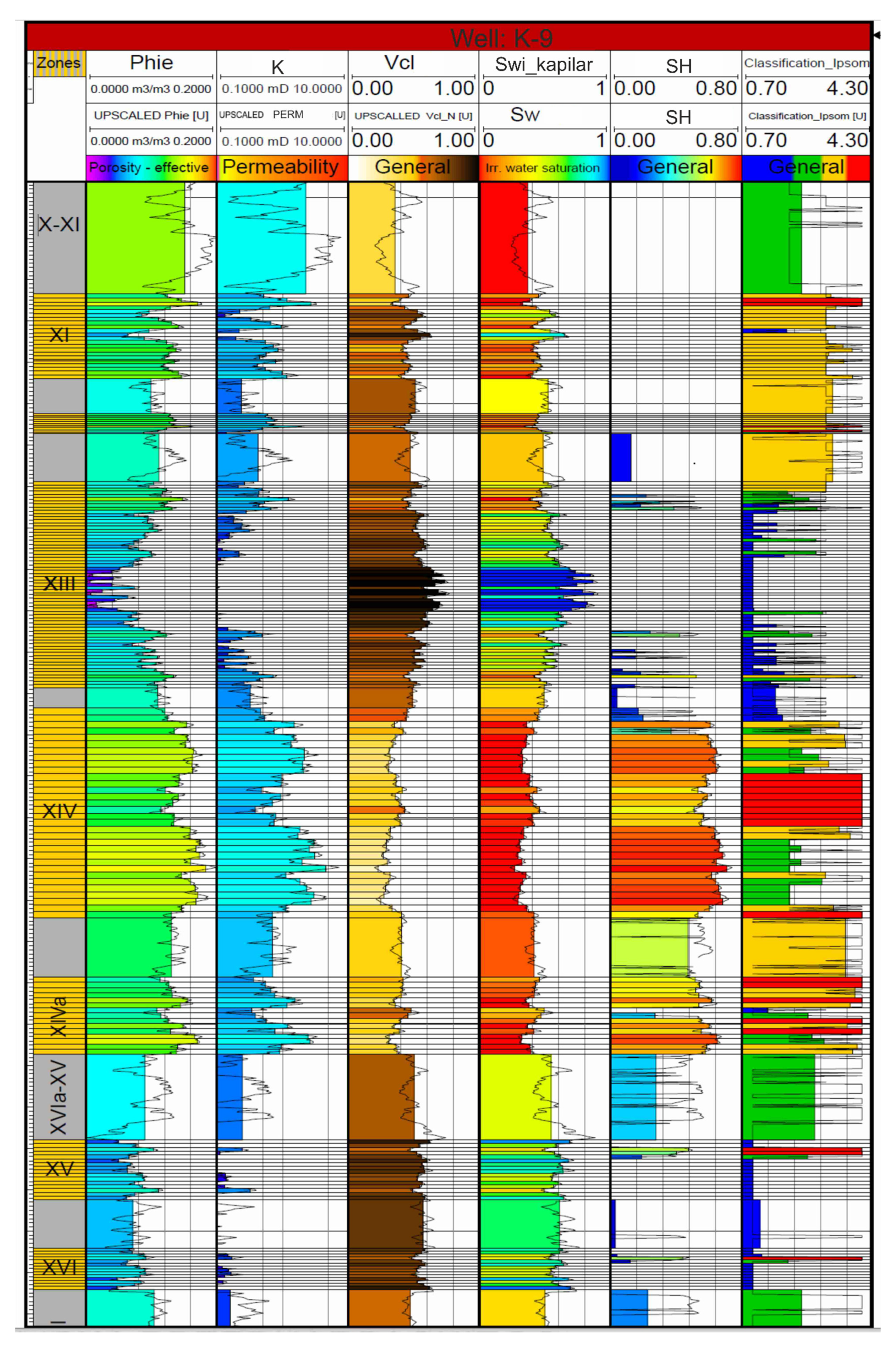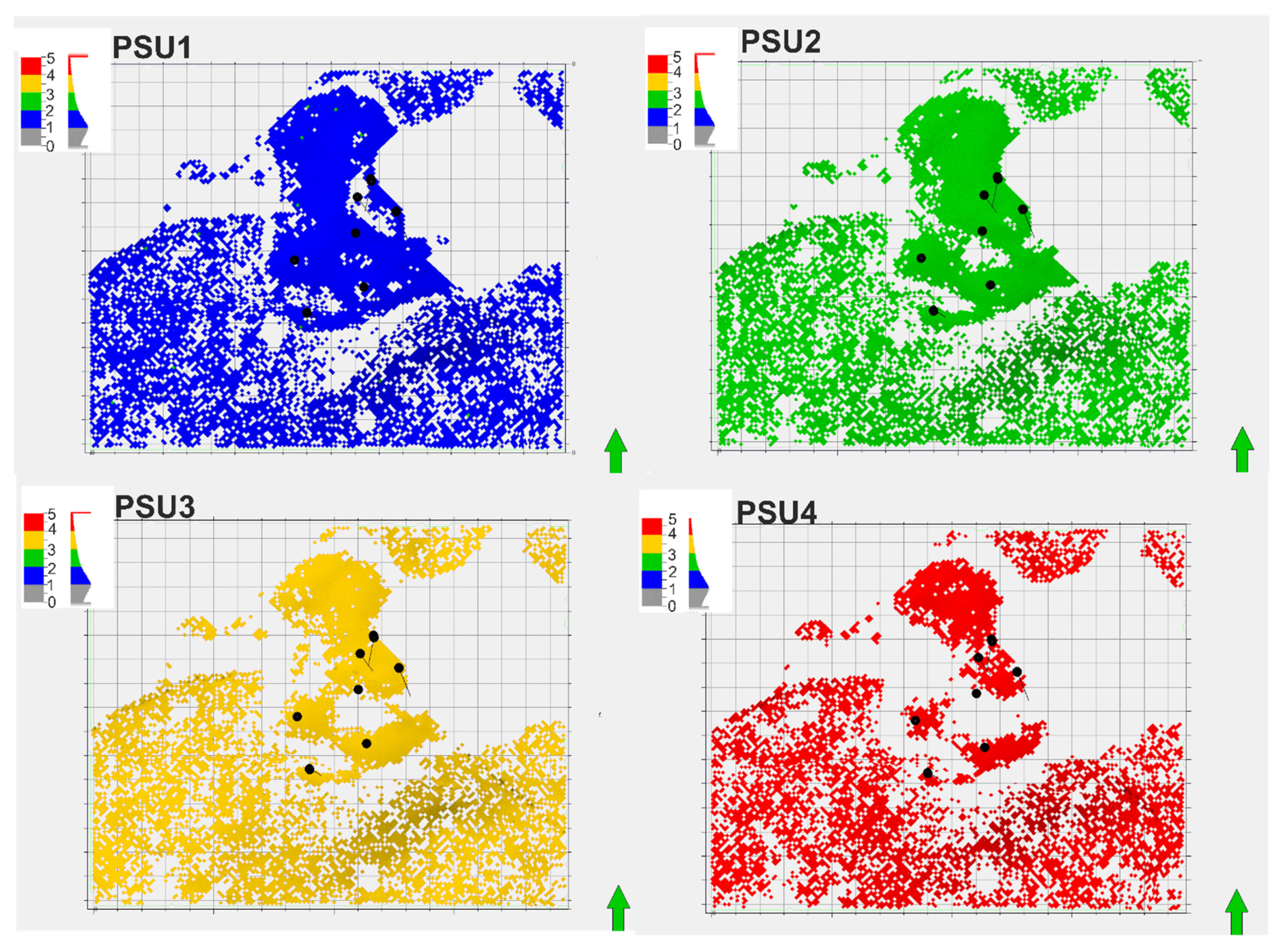Artificial neural networks based on the Kohonen [29] algorithm available in Techlog Schlumberger software were used for data classification. The fuzzy logic classification method was chosen. The network was trained on data from the K-19 well and the results validated for K-17. The network dimension of 10 × 10 was assumed. The trained network was applied to the wellbores K-17, K-18, K-20, K-21K, K-25K, and K-27.

In three archival wells where only three well logs (GR, NPHI, and Rt) were available, the supervised neural network method was used, with the reference to PSUs from well K-19. Despite that fact, the identified PSU groups corresponded to these from new wells, where six input data were used.

Table 2. Average values of petrophysical parameters for individual groups.

	Units	PSU 1. Mudstone/Claystone with Higher Carbonate Content		PSU 2. Porous Sandstone, Mostly Water Saturated		PSU 3. Mudstones Mostly Water-Saturated		PSU 4. Gas-Saturated Shaly-Sands/ Mudstones
Variables		Mean	Variance	Mean	Variance	Mean	Variance	Mean	Variance
Compressional Slowness	μs/m	326.329	28.985	322.360	36.055	339.215	24.054	323.570	51.090
Bulk Density	g/cm3	2.495	0.000	2.362	0.001	2.455	0.001	2.444	0.001
Gamma Ray	API	106.158	8.848	83.506	43.401	104.500	20.555	96.040	17.988
Formation Resistivity	ohm.m	3.661	0.012	2.870	0.583	3.248	0.069	3.973	0.084
Neutron Porosity		0.263	0.000	0.243	0.001	0.283	0.000	0.243	0.000
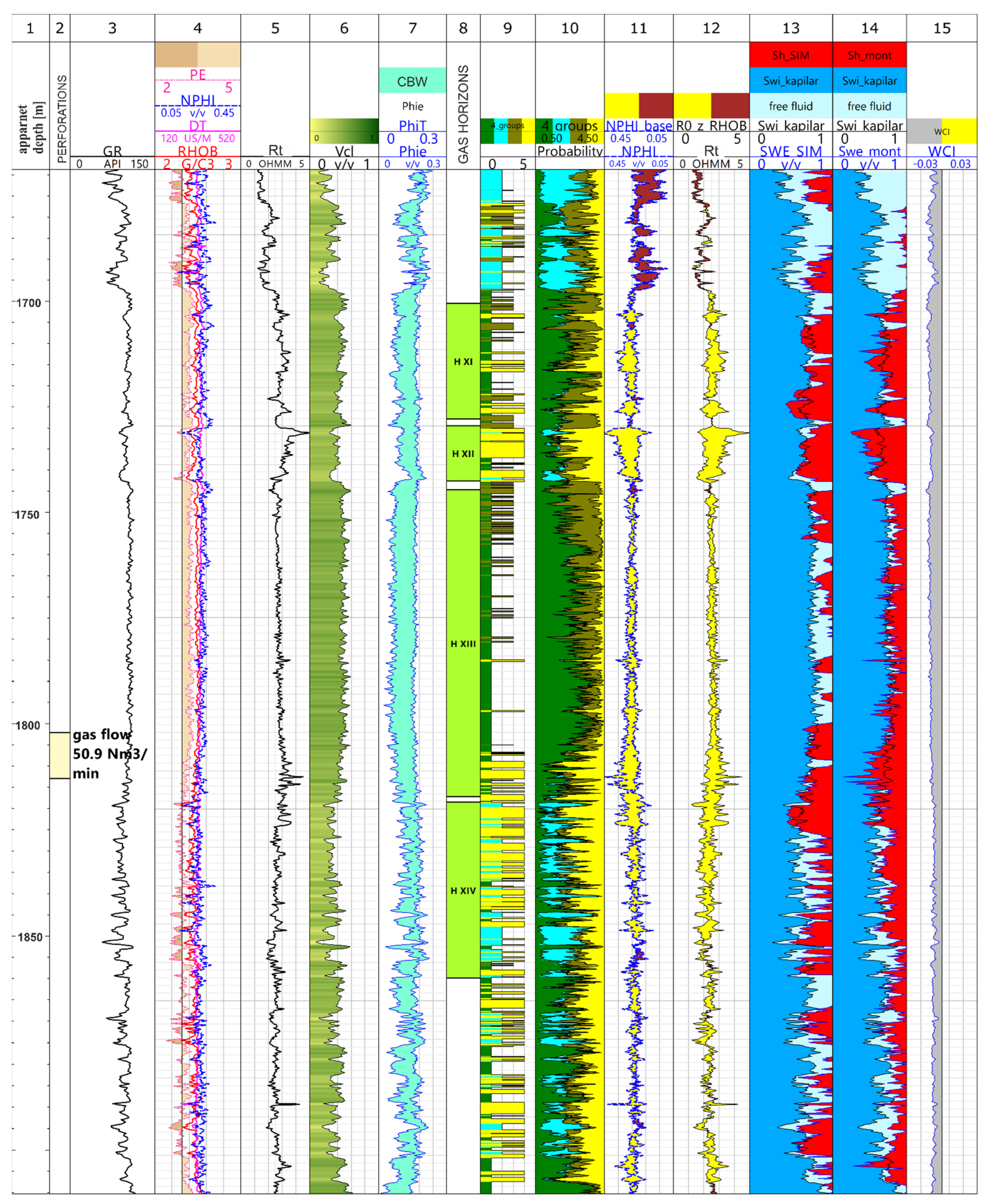
Photoelectric Factor	b/elec	3.182	0.009	2.711	0.009	3.127	0.008	2.971	0.006

presents the mean values of the input data within the four PSUs and descriptions of their petrophysical properties.

PSU 1 represents claystone and mudstones with carbonates, sediments with high clay-bound water content, and an average bulk density of 2.5 g/cm³. This group was comparable to PSU 3 (mudstone); however, the values of neutron porosity for the first group were lower, and the bulk density and resistivity were higher. This was due to the admixture of carbonates present in this electrofacies. XRD measurements indicated between 20 and 30% of carbonates (calcite and dolomite) for this group, which is a group of sediments that constitute sealing layers; it has low effective porosity and is almost impermeable. However, the analysis of high resolution microresistivity logs from well K-19 showed several-meters-thick interbeds of gas-saturated sandstones present within this group of sediments. Unfortunately, these layers were too thin to be properly resolved by conventional well logs. A petrophysical approach to interpretation of this thin-bed formation required the use of high-resolution logs [30,31,32,33,34,35]. At this stage of interpretation, PSU 1 was treated as a sealing unit, as applied methods of interpretation did not allow the hydrocarbon potential of this unit to be properly estimated. The photoelectric factor values were the highest for this group, on average 3.18 b/elec. PSU 2 corresponded to porous sandstone or sandstone/mudstone heterolites. The average gamma ray value for this group was 83.5 API. The bulk density values in this group were the lowest, on average 2.36 g/cm³. The average value of the photoelectric factor was equal to 2.71 b/elec. Average neutron porosity was 0.24. However, the resistivity of this group was very low at 2.87 ohm.m, which suggests that sandstones were mostly water saturated or were in the transition zone with the presence of both gas and water. This unit does not constitute the dominant group associated with gas accumulation. Effective porosity of sandstone layers was high and reached up to 23%. PSU 3 consisted of siltstones/mudstone with the highest neutron porosity of 0.28, compressional slowness value of 339 us/m, and an average resistivity equal to 3.2 ohm.m. These features may suggest that mudstones are organic-rich. However, the uranium content measurements available in the K-25K and K-21K wells were very low and generally did not exceed 4 ppm. The increase in uranium content did not show a relationship with PSU 3. In that case, this group probably is related to mudstones with high irreducible water content; it also might consist of higher volumes of swelling clays such as smectite [36] and low carbonate content. PSU 4 corresponded to layers with the highest hydrocarbon potential. It was characterized by the highest resistivity values of 3.97 ohm.m; the average value of neutron porosity was 0.24 and was similar to that of sandstones of PSU 2. The average gamma ray was 96 API, higher than for sandstones (83.5 API) and lower than for mudstones PSU 3 (104.5 API). The intervals corresponding to PSU 4 coincided with the intervals where calculated water saturation was low. PSU 3 and 4 showed similar parameters, both representing mudstones, but low values of neutron porosity and high values of formation resistivity definitely indicate gas saturation in PSU 4. These petrophysical interpretation results were used in Petrel to model the spatial distribution of clay volume, effective porosity, and hydrocarbon saturation (SH_FIN) within defined PSUs.

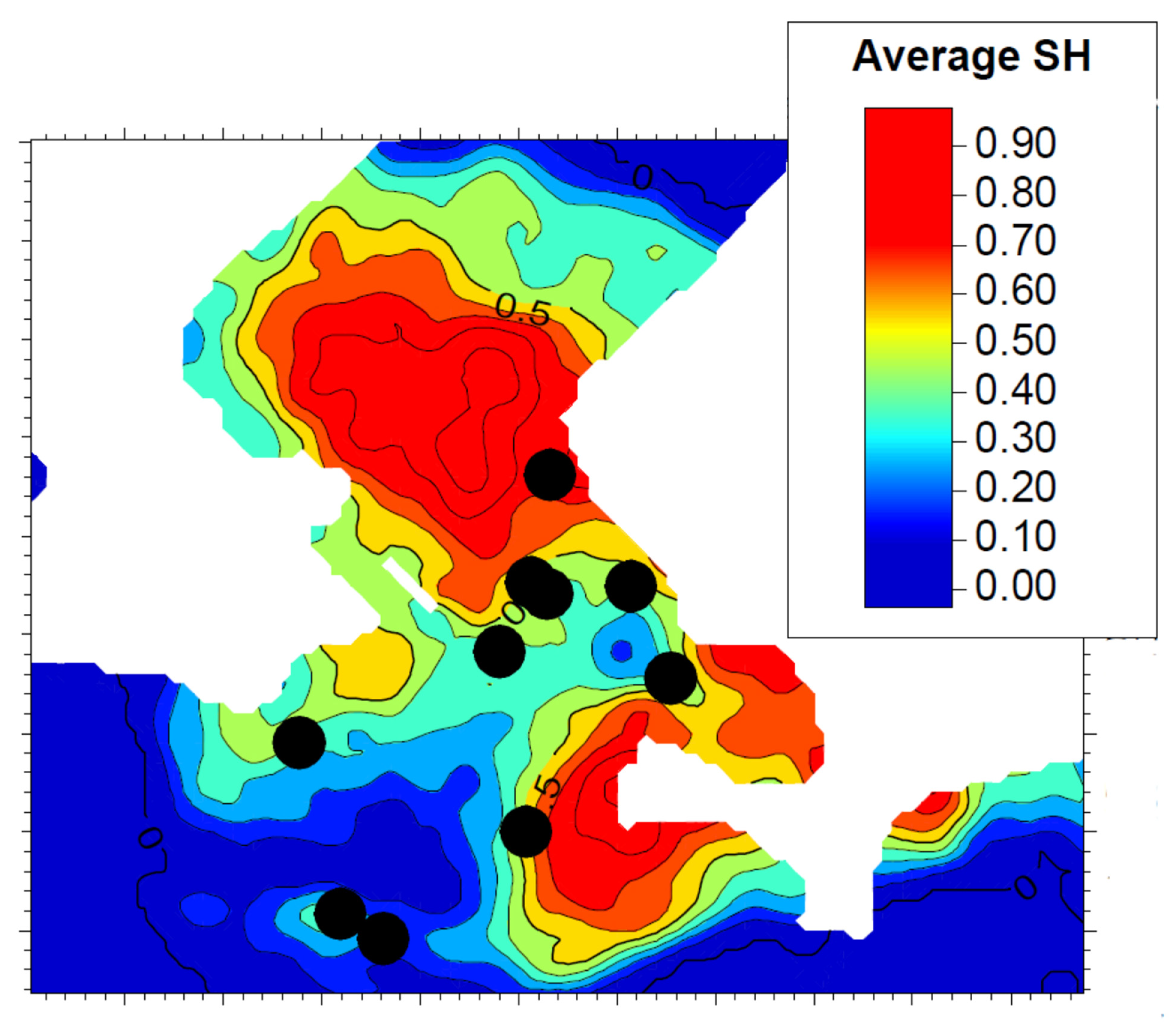
2.7. Spatial Distribution of Petrophysical Parameters

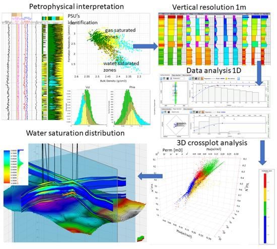
The spatial distribution of facies or petrophysical (clay volume, porosity, permeability, hydrocarbon saturation), geomechanical, and geochemical parameters can be presented through 3D models. Recognition of the variability of reservoir properties within the research area (e.g., a gas field) is an important part of hydrocarbon exploration. On the basis of spatial distributions or maps of individual parameters, one can make a decision that helps to minimize the exploitation costs and maximize production. The maps of the reservoir properties in the gas field, in addition to the structural model, are the basic elements of planning the exploration works, carrying out the calculations of resources, and preparing development projects for the discovered hydrocarbon accumulation. In addition to planning the location of boreholes, the spatial form of mapping the parametric variability of the analyzed reservoir also permits the selection of the well-type (vertical, horizontal). In order to spatially distribute the results of the PSU classification obtained in the profiles of the analyzed boreholes, a number of realizations were generated to reduce the geological uncertainty of the model assessment for the petrophysical PSUs, porosity, and hydrocarbon saturation model. The first stage of work was related to the construction of the structural model. The authors used the structural model created by K. Sowiżdzał. In the next step, definition of the vertical cell size based on the vertical heterogeneity of the log resolution was established. High resolution increased the probability of capturing important changes in reservoir parameters. Applying modern methods of data grouping also allowed us to capture details related to the reservoir and variability of petrophysical properties revealed in the wellbore profiles.

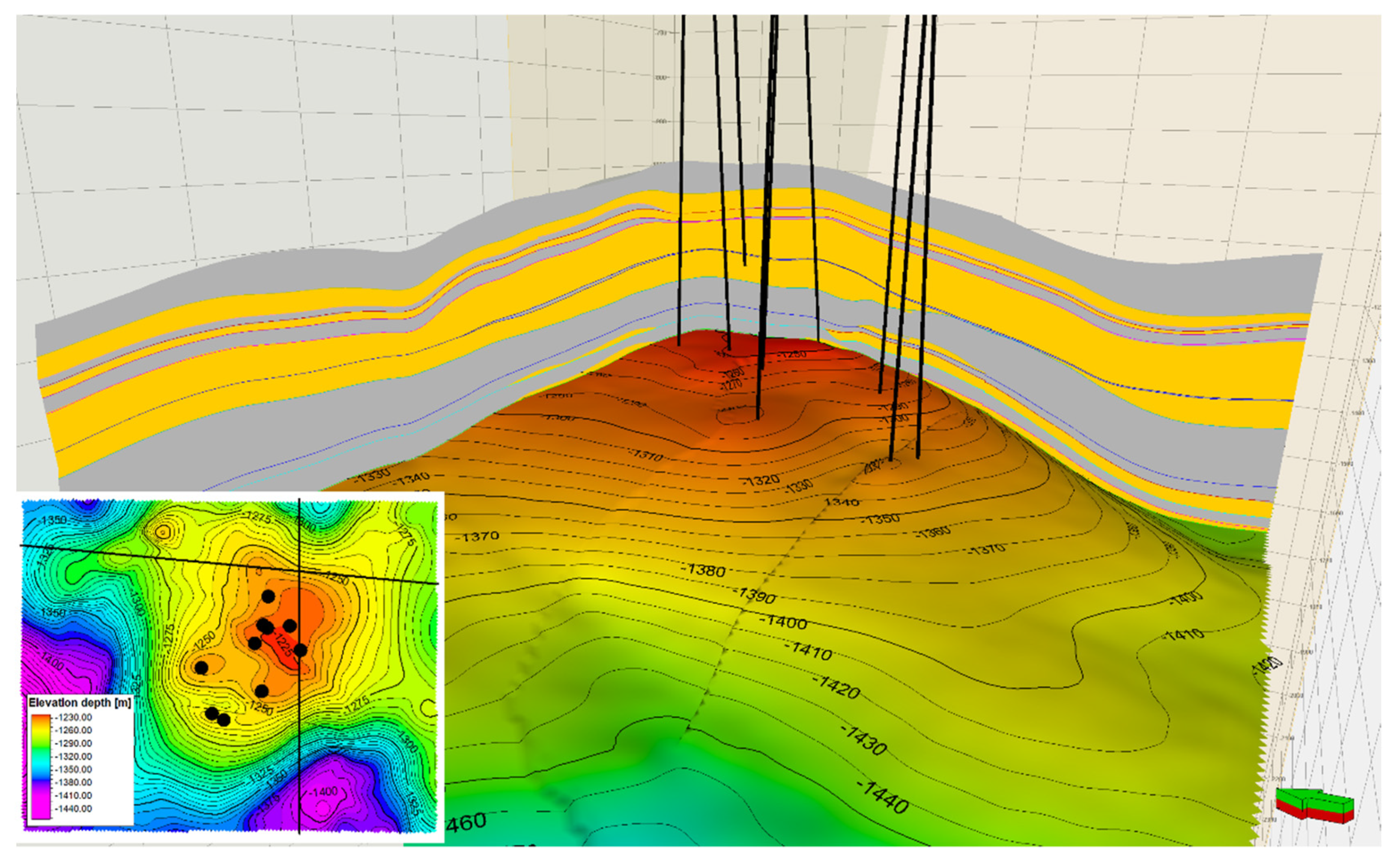
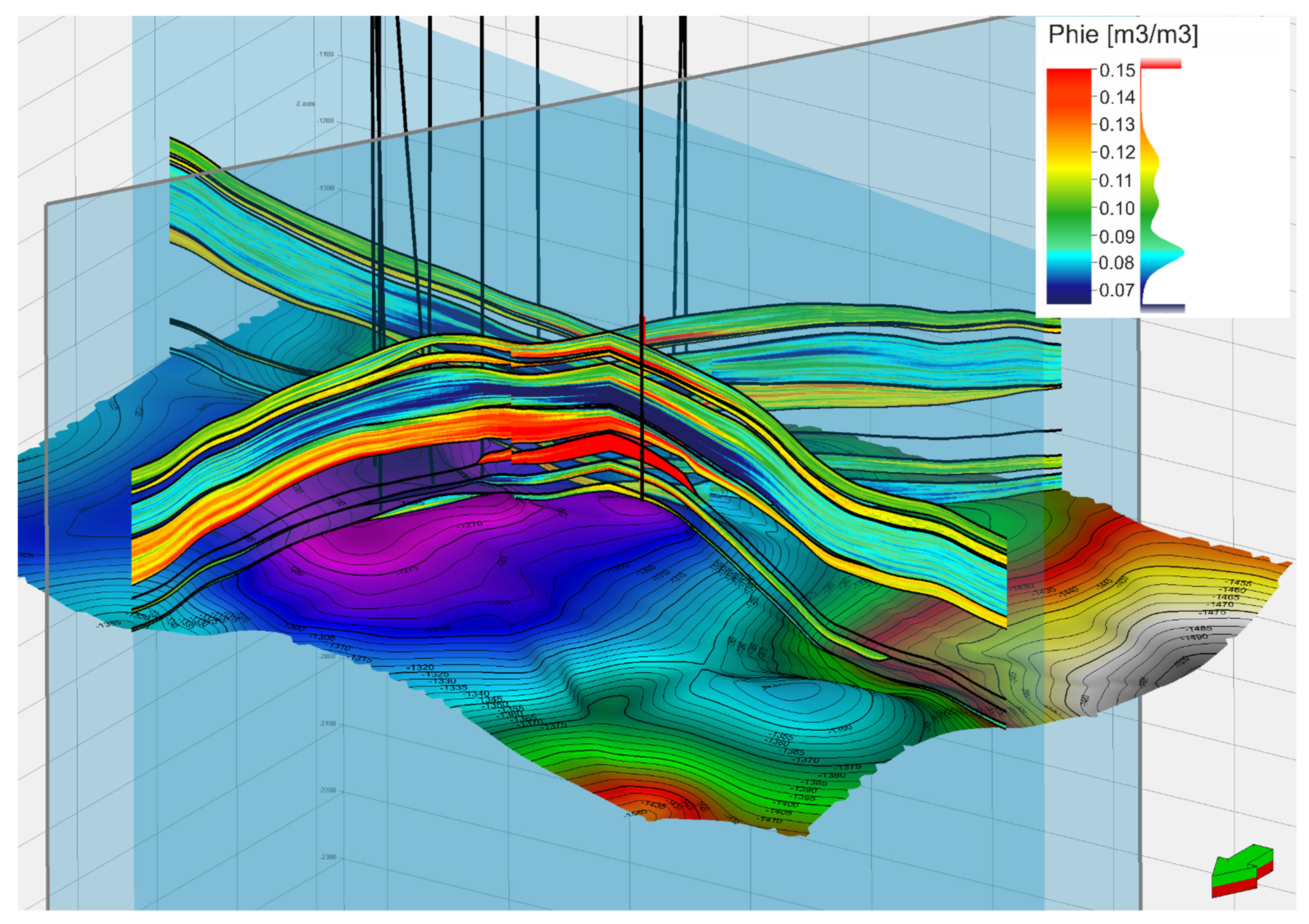
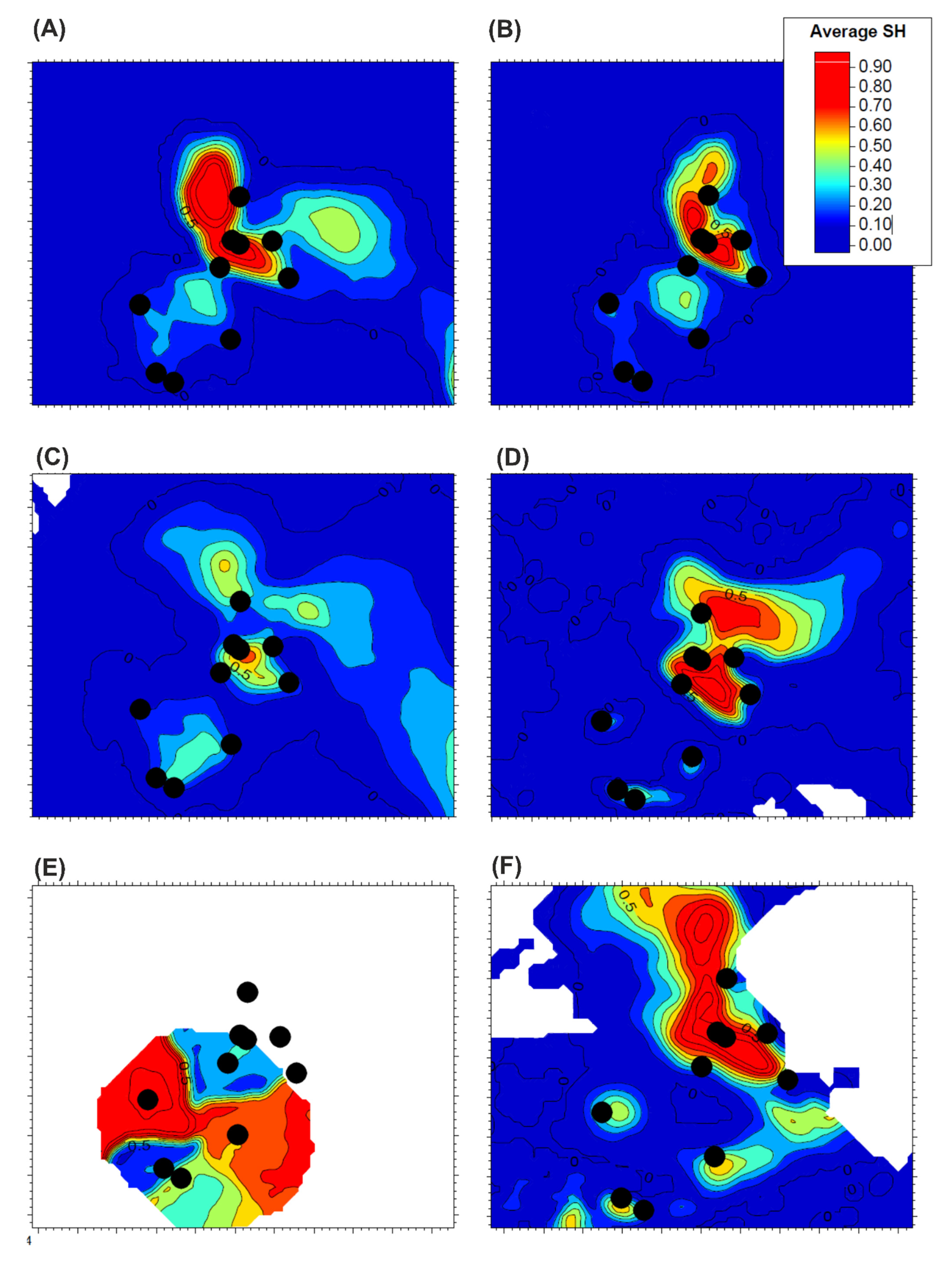
The final structural model consisted of seven gas-bearing horizons (marked in yellow) separated by layers that had not been subjected to the spatial modeling process (gray layers) (Figure 5). Due to the thin-bed nature of the Miocene deposits, the individual gas-bearing horizons, being the subject of the analysis, had an average vertical resolution of the grid of about 1 m (Figure 6). The total number of model cells in the intervals covered by the analysis was 6,925,200 (

Table 3. Quantitative characteristics of the individual intervals that were the subject of the research.

Horizon	Average Thickness (m)	Number of Grid Cells
XI	22.2	875,600
XII	9.6	398,000
XIII	64.5	2,587,000
XIV	31.8	1,273,600
XIVa	14	597,000
XV	15.4	636,800
XVI	13.5	557,200

).

The final model showed the spatial distribution of individual petrophysical groups through the variability of reservoir parameters in each PSU group. The range of variability for reservoir parameters in each PSU group was defined based on the interpretation performed for the boreholes (

Table 4. The range of variability of the most important reservoir properties for each PSU group.

PSU	Vcl (v/v)	Phie (v/v)	K (mD)	Swi_Kapilar (v/v)	SH-Hydrocarbon Saturation (1-Sw)
1	0.55–0.7	0.03–0.05	0.01–0.1	0.8–0.9	1—sealing unit
2	0.1–0.35	0.15–0.23	10–20	0.3–0.4	SH
3	0.4–0.5	0.05–0.12	0.05–1	0.4–0.6	SH
4	0.35–0.45	0.08–0.15	0.1–10	0.4–0.5	SH

).

For hydrocarbon saturation, no predefined values for each group were applied (except PSU1, which was treated as a sealing unit), but the continuous curve of SH was used. First, the data analysis was carried out (defining the physical values of the modeled parameter) and the parametric modeling process itself.

2.8. Defining the Direction and Extent of Variograms

The analysis of the semivariogram function was carried out on the basis of a graph in which the x-axis showed the distance between the tested locations of the analyzed variable, the y-axis corresponded to 12 variances (i.e., semivariances), and the points were the values of the experimental variogram. Variogram analysis consists of adjusting the type of theoretical model to the nature of the variability observed in the data population, represented by the points of the experimental variogram by determining a number of parameters. The results are applied at the stage of parametric modeling of individual parameters

2.9. Parametric Modeling

At the parametric modeling stage, for each gas-bearing horizon, the results of data analyses carried out in the previous step were applied, and a computational algorithm was selected. For clay volume, effective porosity, and permeability, a stochastic Gaussian random function simulation algorithm was selected.

For each of the modeled parameters, 25 equally probable realizations of the spatial distribution were generated, which were finally subjected to the averaging process.

Parametric modeling results were verified by comparison of the histograms of the input data (well logs) with the data averaged in the resolution of the grid (upscaled logs) and models.

Based on the parametric models constructed in the previous step (Phie, Vcl), the reconstruction of the spatial distribution of reservoir parameters within the analyzed gas-bearing horizons was carried out. The procedure of spatial electrofacies classification consisted of the application of parametric models and the classifier formula in the form of an interpretation of electrofacies (the results of the PSU classification carried out with the use of the IPSOM module on well log data). The classification algorithm defined the membership of each grid cell to the PSU showing the highest degree of probability, also showing the value of this probability.

Finally, reconstruction of the spatial distribution of hydrocarbon saturation (SH) was performed. Neural networks were used to recreate the meta-attributes (pseudo-attributes) of this parameter (parameter with nonphysical values). Even so, pseudo-attributes can still be valuable information of a qualitative nature. The quantitative nature of the data was ensured by the procedure related to data analysis. At this stage, ranges of values (minimum, average, maximum) and a distribution curve for the value of a given parameter were defined based on information from the borehole.

3. Results

The results of well log data interpretation of the selected wells and spatial distribution of reservoir properties and PSUs in the form of property maps are presented below.

Table 5. Description of mnemonics and interpretation results of individual paths from Figure 6 and Figure 7.

Track Number	Mnemonic	Description
1	MD	Measured depth
2	perforations	Perforated interval
3	GR	Normalized gamma ray
4	PE, NPHI, DT, RHOB	Normalized: photoelectric factor, neutron porosity, compressional slowness, bulk density
5	Rt	Normalized formation resistivity
6	Vcl	Clay volume
7	Phie, PhiT, PHIE	Effective porosity, total porosity, and laboratory-measured porosity (PHIE)
8	XI, XII, XII, XIV	Horizon names
9	PSU groups	1—claystones/mudstones, 2—sandstones, 3—mudstones, 4—mudstones with high hydrocarbon potential
10	probability	Probability of occurrence of each facie at a specific depth
11	NPHI_base, NPHI	Qualitative method of detection of gas-saturated zones based on modified Passey’s method: yellow—gas-saturated zones; brown—water saturated zones
12	Rt, R0_RHOB	Qualitative method of detection of gas-saturated zones based on difference between RT and R0
13	Swe_SIM, Swi_kapilar	Effective water saturation calculated from the Simandoux [37] formula (Swe_SIM), irreducible water saturation—Swi_kapilar
14	Swe_mont, Swi_kapilar	Effective water saturation calculated from the modified Montaron equation (Swe_mont), irreducible water saturation—Swi_kapilar
15	WCI	Water connectivity index

is a detailed description of each column’s contents from Figure 7 and Figure 8.

Calculated water saturation from the modified Montaron method indicates higher gas saturation in sandstones intervals comparing to Simandoux results. Simandoux model is basically dedicated shaly formations but if there is high variability of shale volume content as it is in heteroliths reservoirs there will be a necessity to subdivide reservoir into high number of thin beds and use different saturation model in each kind of facie, which may be confused and will lead to discontinuity, rapid changes in water saturation profile. Additionally, Simandoux method is only resistivity sensitive, it does not account for i.e., neutron porosity or bulk density changes, which may lead to underestimating water saturation in intervals where increasing resistivity is not related to the presence of hydrocarbon, for example, higher calcite content. Moreover, if there is little contrast or no contrast between gas saturated and water saturated zone Simandoux model will consequently show gas saturation through the whole interpreted interval or water saturation depending on assumed claystone resistivity. Involving RHOB or NPHI logs at stage of Sw calculation will give extra indicator that may confirm or not the presence of gas. The more input data taken into account, the lower the uncertainty of the calculated Sw. The advantage of Montaron model is also the fact of using measured “in situ” well logs as an input. The method does not rely on calculated parameters as Vcl or Phie that may have a high level of uncertainty. Via spatial propagation of petrophysical properties from boreholes, one can determine the favorable areas potentially gas saturated. The distribution of reservoir parameters was performed within the defined PSU’s. Moreover, even the sole spatial propagation of PSU’s might be a good qualitative hydrocarbon indicator, as PSU 4 is highly related to existing gas accumulations. This may give a first look at the perspective of the area before petrophysical interpretation is carried out.

High resolution of the model allowed for more reliable spatial variability of the individual layers that constitute the Miocene formation. Figure 9 present the effective porosity within the modeled horizons while Figure 10 show the spatial distribution of PSUs in horizon XV.

Figure 11 and Figure 12 present the distribution of the hydrocarbon saturation (SH) in individual gas-bearing horizons. Finally, the works presented in this paper allowed for reconstruction of hydrocarbon saturation in the analyzed area and the generation of maps of average values of this parameter for each of the analyzed gas horizons.

The analyses of the results presented in the form of maps of average hydrocarbon saturation indicate best perspectivity for horizons XV and XVI showed high hydrocarbon saturation in the north-west part of the anticline; in addition, the thickness of several dozen meters make these horizons attractive for the future exploitation. Additionally, the morphology of Precambrian basement constitutes the traps which preserve hydrocarbons from migration. In turn horizon XIVa showed high hydrocarbon saturation in the central and south part of the evaluated gas field, but the coverage of this horizon was significantly limited by the lithological changes, the increase in clay volume, and decrease in effective porosity. In addition, horizons XI and XIV indicate gas saturation in the northern and north-east part of the anticline that pointing out that area favorable for the exploration and drilling works. Horizon XIII was dominated by PSU 1 with low porosity and permeability. Detail interpretation of perspectives of this horizon requires the availability of high resolution well logs and much higher vertical resolution of the model.

4. Discussion

The interpretation of the Miocene multihorizons gas field allowed us to characterize the reservoir parameters of sandy-clay and silt sediments, in which most gas accumulation can be observed. Simultaneously, qualitative methods of detecting gas-saturated intervals were proposed based on well log data. An alternative modified connectivity equation for shaly-sands was applied to calculate water saturation. The model enabled us to calculate the value of Sw in the deposits formed as mudstones or sandstones with clay content higher than 35%, without the need to determine Archie’s saturation exponent (n). This method is mainly based on the results of well log data that reflect the reservoir properties. The results of the Sw estimation are consistent; water saturation based on the Montaron method shows correlation with the Sw obtained from the Simandoux equation and clearly indicates intervals with high hydrocarbon potential. However, the Montaron method, which also uses the porosity logs (RHOB or NPHI) in the intervals with low resistivity contrast (LRC) zones, shows lower values of water saturation compared to Sw from the Simandoux equation. This indicates that porosity logs (RHOB, NPHI, DT) could constitute valuable additional input at the stage of water saturation calculation in formations of high clay content. On the basis of the interpretation, it is possible to define the properties of the sediments in which most of the gas accumulation is observed. The effective porosity of shaly gas horizons ranges from 5 to 15%, and the water saturation ranges from 26 to 50%. The effective porosity of these sediments is reduced by the irreducible water, the capillary water (Swi_kapilar), the content of which ranges from 40 to 70%. The qualitative analysis of mudstone and claystone heteroliths classified as PSU 1 did not clearly show the possibility of gas saturation in these formations, as the water saturation coefficient is very high, at 80–90%. However, the detailed analysis of high-resolution microresistivity measurements in the K-19 well confirmed the presence of thin layers of gas-saturated sandstones within these sediments (horizon XI and XIII). Proper calculation of the reservoir parameters within these rare sandstone inserts due to their thin-layer nature requires a separate interpretation approach based on high-resolution microresistivity logs. Moreover, spatial modeling of reservoir parameters within this group of sediments requires a significant increase in the resolution of the model.

Propagation of the petrophysical properties of individual PSU groups was carried out based on the well log interpretation and predefined ranges of variability of reservoir parameter for the individual group. The reconstruction of the spatial distribution of clay volume and porosity was performed with standard parametric modeling procedures using the Gaussian random function simulation stochastic algorithm, while for the two key parameters for this study, PSU grouping and SH hydrocarbon saturation, different approaches were used. The distribution of the classification into PSU groups was carried out by the facies classification procedure, which enabled us to define the membership of each grid cell to the group (1, 2, 3, 4) showing the highest degree of probability of its occurrence. The spatial distribution of hydrocarbon saturation was based on the use of the SH parameter calculated on the basis of the Montaron method and the petrophysical classification of PSU. The results of petrophysical interpretation indicate the presence of hydrocarbons, including those beyond predefined gas horizons. Thus arises the necessity of verification and redefinition of horizon boundaries.

5. Conclusions

Presented work confirmed the nature of gas deposits developed in the Miocene formation. As was noted in the previous works, the favorable conditions for gas accumulations provide the thin layers of sandstones and mudstones sealing by the laminas of impermeable claystones with admixtures of calcite and dolomite. The thick massive sandstones with effective porosity of 25–29% usually cannot keep hydrocarbons as there are not enough thick impermeable layers that will prevent the hydrocarbons from migration. Although the existing gas accumulation in the heteroliths of basin plain deposits have moderate reservoir properties porosity of several percent and higher level of clay volume, their thickness can reach even 100 m. That makes these multihorizons, consist of thin laminas of gas saturated mudstones and sandstones layered by impermeable claystone, economically important. The perforations documented the gas flow from these horizons of several dozen cubic meters per minute. Unfortunately, we still suffer from the small amount of laboratory measurements performed on core samples. There is need for an accurate recognition of lithological composition of these horizons that may be provide both by the X-ray diffraction tomography measurements of core sample and new well logging profiling. The most important from exploration point of view become the accurate calculation and core calibration of irreducible and free fluid volume. Miocene deposits are often thin-bedded thus new well logging technology should be used to collect data with higher resolution. Very useful in pay zone detection could be measurements of vertical (Rv) and horizonal (Rh) resistivities. Xaminer Multicomponent Induction (MCI) is dedicated to evaluation anisotropic thin-bedded formations and is a tool that measures formation resistivity both vertically and horizontally at different depths of investigation. When run with a directional tool, it also provides structural dip and azimuth. However, horizontal microresistivity can also be measured with the use of imagers of borehole walls (XRMI). The paper shows that even using basic well logs we can roughly assess the potential of Miocene heteroliths. New looks at conventional well log data in combination with laboratory measurements and propagation within the reservoir allowed indication of potentially gas saturated areas. We can deal with low resistivity contrast between gas and water saturated intervals by involving other available logs, usually dedicated porosity calculation (NPHI, DT, RHOB), at the stage of water saturation calculation.

References

1. Dziadzio, P.; Liszka, B.; Maksym, A.; Stryszak, G. Środowisko sedymentacji utworów miocenu autochtonicznego w brzeżnej strefie Karpat, a interpretacja geologiczno-złożowa w obszarze Husów–Albigowa–Krasne. Nafta-Gaz 1997, 53, 407–414. (In Polish) [Google Scholar]
2. Dziadzio, P. Depositional sequences in Badenian and Sarmatian deposits in the SE parts of the Carpathian Foredeep (SE Poland). Przegląd Geol. 2000, 48, 1124–1138. (In Polish) [Google Scholar]
3. Porębski, S.J.; Pietach, K.; Hodiak, R.; Steel, R.J. Origin and sequential development of Upper Badenian-Sarmatian clinoforms in the Carpathian Foredeep Ba sin, SE Poland. Geol. Carpathica 2002, 54, 119–136. [Google Scholar]
4. Kurovets, I.; Prytulka, G.; Shpot, Y.; Peryt, T.M. Middle Miocene Dashava Formation sandstones, Carpathian Foredeep. Ukr. J. Pet. Geol. 2004, 27, 373–388. [Google Scholar] [CrossRef]
5. Mastalerz, K.; Wysocka, A.; Krzywiec, P.; Kasiński, J.; Aleksandrowski, P.; Papiernik, B.; Ryzer-Siupik, J. Miocene succession at the Ryszkowa Wola High (Sieniawa-Rudka area), Carpathian Foredeep Basin: Facies and stratigraphic interpretation of wellbore and 3D seismic data. Przegląd Geol. 2006, 54, 333–342. (In Polish) [Google Scholar]
6. Pietsch, K.; Porębski, S.J.; Marzec, P. The use of seismostratigraphy for exploration of Miocene gas-geaing reservoirs in the NE part of the Carpathian Foreland Basin (Poland). Geologia 2010, 36, 173–186. (In Polish) [Google Scholar]
7. Oszczypko, N.; Krzywiec, P.; Popadyuk, I.; Peryt, T. Carpathian Foredeep Basin (Poland and Ukraine): Its sedimentary, structural, and geodynamic evolution. In The Carpathians and Their Fore Land: Geology and Hydrocarbon Resources; Golonka, J., Picha, F.J., Eds.; American Association of Petroleum Geologists: Tusla, OK, USA, 2006. [Google Scholar]
8. Montaron, B. Connectivity Theory—A new approach to modeling Non-Archie rocks. Petrophysics 2009, 50, 102–115. [Google Scholar]
9. Passey, Q.; Creaney, S.; Kulla, J.; Moretti, F.; Stroud, J. A pratical model for organic richness from porosity and resistivity logs. Am. Assoc. Pet. Geol. Bull. 1990, 74, 1777–1794. [Google Scholar]
10. Bowman, T. Direct Method for Determining Organic Shale Potential from Porosity and Resistivity Logs to Identify Possible Resource Plays Mantle Oil & Gas; LLC AAPG Annual Convention & Exhibition: New Orleans, LA, USA, 2010. [Google Scholar]
11. Dudek, J.; Dudek, L.; Klimek, P. Badania ekshalacji gazu w rejonie złoża Przeworsk. In Proceedings of the Geopetrol 2004: Konferencja Naukowo-Techniczna nt. Efektywne Technologie Poszukiwania i Eksploatacji Złóż Węglowodorów, Zakopane, Polish, 20–23 September 2004. [Google Scholar]
12. Dudek, J.; Zaleska-Bartosz, J. Ocena Możliwości Realizacji Inwestycji Budowlanych na Terenie Złoża Przeworsk, w Kontekście Występowania Zagrożeń Ekshalacji Gazu Ziemnego. Nafta-Gaz 2011, 7, 463–466. [Google Scholar]
13. Kołodziejak, G. Ocena Możliwości Minimalizacji Zagrożeń Powodowanych Ekshalacjami Gazu Ziemnego na Terenie Miasta Przeworsk. Nafta-Gaz 2010, 66, 591–596. [Google Scholar]
14. Myśliwiec, M. Exploration for gas accumulations in the Miocene deposits of the Carpathian Foredeep using direct hydrocarbon indicators—Verification of anomalies (southern Poland). Prz. Geol. 2004, 52, 307–314. [Google Scholar]
15. Archie, G.E. The electrical resistivity log as an aid in determining some reservoir characteristics. J. Pet. Technol. 1942, 1, 55–62. [Google Scholar] [CrossRef]
16. Montaron, B. A Quantitative Model for the Effect of Wettability on the Conductivity of Porous Rocks SPE. In Proceedings of the SPE Middle East Oil and Gas Show and Conference, Manama, Bahrain, 11–14 March 2007. [Google Scholar] [CrossRef]
17. Jarzyna, J.; Krakowska, P. Dobór Parametrów Petrofizycznych Węglanowych Skał Zbiornikowych w Celu Podwyższenia Dokładności Wyznaczenia Współczynnika Nasycenia Wodą. Nafta-Gaz 2010, 7, 547–556. [Google Scholar]
18. Lee Myung, W. Connectivity Equation and Shaly-Sand Correction for Electrical Resistivity; Scientific Investigations Report 2011-5005; Unites States Geological Survey: Liston, VA, USA, 2011.
19. Peeters, M.; Holmes, A. Review of Existing Shaly-Sand Models and Introduction of a New Method Based on Dry-Clay Parameters. Petrophysics 2014, 55, 543–553. [Google Scholar]
20. Puskarczyk, E.; Jarzyna, J.; Porębski, S.J. Application of multivariate statistical methods for characterizing heterolithic reservoirs based on wireline logs—Example from the Carpathian Foredeep Basin (Middle Miocene, SE Poland). Geol. Q. 2015, 59, 157–168. [Google Scholar]
21. Puskarczyk, E. Artificial neural networks as a tool for pattern recognition and electrofacies analysis in PolishPalaeozoic shale gas formations. Acta Geophys. 2019, 67, 1991–2003. [Google Scholar] [CrossRef] [Green Version]
22. Moss, B.; Seheult, A. Does principal component analysis have a role in the interpretation of petrophysical data? In Proceedings of the 28th Annual Logging Symposium Transactions, Society Professional Well Log Analysts, London, UK, 29 June–2 July 1987. [Google Scholar]
23. Szabó, N.P.; Dobroka, M.; Kavanda, R. Cluster analysis assisted float-encoded genetic algorithm for a moreautomated characterization of hydro-carbon reservoirs. Intell. Control Autom. 2013, 4, 362–370. [Google Scholar] [CrossRef] [Green Version]
24. Wawrzyniak-Guz, K.; Puskarczyk, E.; Krakowska, P.I.; Jarzyna, J.A. Classification of Polish shale gas formations from Baltic Basin, Poland based on well logging data by statistical methods. In Proceedings of the International Multidisciplinary Scientific GeoConference SGEM, Albena, Bulgaria, 30 June–6 July 2016; pp. 761–768, ISSN 1314-2704. ISBN 978-619-7105-57-5. [Google Scholar]
25. Kohonen, T. Self-Organizing Maps; Springer: Berlin/Heidelberg, Germany, 2001. [Google Scholar] [CrossRef]
26. Odesanya, I.; Ogbamikhumi, A.; Azi, O.S. Well Log Analysis for Lithology Identification Using Self-Organizing Map (SOM). Int. J. Res. Appl. Phys. 2016, 2, 25–32. [Google Scholar]
27. Liu, Y.; Weisberg, H.R.; Mooers, N.K.C. Performance evaluation of the self-organizing map for feature extraction. J. Geophys. Res. Ocean. 2006, 111, 1–14. [Google Scholar] [CrossRef]
28. Thomson, E.R.; Emery, W.J. Data Analysis Methods in Physical Oceanography, 3th ed.; Elsevier: Amsterdam, The Netherlands, 2014; ISBN 978-0-12-387782-6. [Google Scholar]
29. Kohonen, T. Self-Organized Formation of Topologically Correct Feature Maps. Biol. Cybern. 1982, 43, 59–69. [Google Scholar] [CrossRef]
30. Nooh, A.Z.; Moustafa, E.A.A. Comparison of Quantitative Analysis of Image Logs for Shale Volume and Net to Gross Calculation of a Thinly Laminated Reservoir between VNG-NERGE and LAGIA-EGYPT. Egypt. J. Pet. 2017, 26, 619–625. [Google Scholar] [CrossRef]
31. Eshimokhai, S.; Akhirevbulu, O.E.; Osueni, L. Evaluation of Thin Bed Using Resistivity Borehole and NMR Imaging Techniques. Ethiop. J. Environ. Stud. Manag. 2012, 4, 96–102. [Google Scholar] [CrossRef] [Green Version]
32. Ruhovets, N.; Rau, R.; Samuel, M.; Smith, H.; Smith, M., Jr. Evaluating Thinly Laminated Reservoirs Using Logs with Different Vertical Resolution Halliburton Logging Services; Pennsylvania State University: State College, PA, USA, 2016; Available online: http://sp.lyellcollection.org/ (accessed on 1 March 2021).
33. Saxena, K.; Tyagi, A.; Klimentos, T.; Morriss, C.; Mathew, A. Evaluating Deepwater Thin-Bedded Reservoirs with Rt Scanner; Petromin: Kuala Lumpur, Malaysia, 2006. [Google Scholar]
34. Kusuma, D.P.; Audinno, R.T.; Pratama, I.P.; Halim, A. Integrated Analysis of The-Low Resistivity Hydrocarbon Reservoir in the “S” Field. In Proceedings of the Conference: Indonesian Petroleum Association, Fortieth Annual Convention & Exhibition, Jakarta, Indonesia, 25–27 May 2016. [Google Scholar] [CrossRef]
35. Lis-Śledziona, A. Multiscale evaluation of a thin-bed reservoir. Geol. Geophys. Environ. 2021, 47, 5–20. [Google Scholar] [CrossRef]
36. Przelaskowska, A.; Łykowska, G.; Klaja, J.; Kowalska, S.; Gąsior, I. Application of the cation exchange capacity parameter (CEC) to the characterization of the swelling capacity of lower Paleozoic, Carpathian Flysch and Miocene Carpathian Foredeep clay rocks. Nafta-Gaz 2015, 6, 384–389. [Google Scholar]
37. Simandoux, P. Dielectric measurements in porous media and applications in Shaly formations. In Revue de L’institute Francais de Petrole-SPWLA English Translation Volume Shaly Sand; SPWLA: Huston, TX, USA, 1982. [Google Scholar]
Figure 1. (A) Scheme of a typical deposit complex in the Miocene formations of the Carpathian Foredeep. (B) Well log identification of different Miocene sedimentary environments.
Energies 15 01890 g001
Figure 2. Interpreted gas deposit formed as anticline with the location of wellbores.
Energies 15 01890 g002
Figure 3. Well log data used in the interpretation of the K-17 well.
Energies 15 01890 g003
Figure 4. (A) Correlation of the measured effective porosity and the bulk density; (B) correlation of laboratory-measured porosity and capillary water content measured by NMR.
Energies 15 01890 g004
Figure 5. Cross-section through the structural model of the analyzed deposit complex (view from the west side) with a location map of the wells and cross-sectional lines.
Energies 15 01890 g005
Figure 6. Well log data (solid black line) averaged at the vertical resolution of the grid.
Energies 15 01890 g006
Figure 7. The results of petrophysical well log interpretation for well K-21K.
Energies 15 01890 g007
Figure 8. The results of petrophysical well log interpretation for well K-27.
Energies 15 01890 g008
Figure 9. Final spatial distribution of effective porosity.
Energies 15 01890 g009
Figure 10. Spatial distribution of PSUs in gas horizon XV.
Energies 15 01890 g010
Figure 11. Maps of average hydrocarbon saturation in gas-bearing horizons: (A) XI, (B) XII, (C) XIII, (D) XIV, (E) XIVa, and (F) XV. White represents areas beyond the lithological barrier of the horizon.
Energies 15 01890 g011
Figure 12. Maps of average hydrocarbon saturation in gas-bearing horizon XVI. White represents areas, beyond the lithological barrier of the horizon (Precambrian basement).
Energies 15 01890 g012