Optimal Placement of Renewable Energy Generators Using Grid-Oriented Genetic Algorithm for Loss Reduction and Flexibility Improvement

Abstract

Optimal planning of renewable energy generator (REG) units helps to meet future power demand with improved flexibility. Hence, this paper proposes a grid-oriented genetic algorithm (GOGA) based on a hybrid combination of a genetic algorithm (GA) and a solution using analytical power flow equations for optimal sizing and placement of REG units in a power system network. The objective of the GOGA is system loss minimization and flexibility improvement. The objective function expresses the system losses as a function of the power generated by different generators, using the Kron equation. A flexibility index (FI) is proposed to evaluate the improvement in the flexibility, based on the voltage deviations and system losses. A power flow run is performed after placement of REGs at various buses of the test system, and system losses are computed, which are considered as chromosome fitness values. The GOGA searches for the lowest value of the fitness function by changing the location of REG units. Crossover, mutation, and replacement operators are used by the GOGA to generate new chromosomes until the optimal solution is obtained in terms of size and location of REGs. A study is performed on a part of the practical transmission network of Rajasthan Rajya Vidyut Prasaran Nigam Ltd. (RVPN), India for the base year 2021 and the projected year 2031. Load forecasting for the 10-year time horizon is computed using a linear fit mathematical model. A cost–benefit analysis is performed, and it is established that the proposed GOGA provides a financially viable solution with improved flexibility. It is established that GOGA ensures high convergence speed and good solution accuracy. Further, the performance of the GOGA is superior compared to a conventional GA.

1. Introduction

An international focus on a cleaner environment has forced utilities to meet increased demand with renewable energy (RE) sources. It is expected that renewable energy sources will contribute almost 50% of the total electrical power generated by 2050. Power generation from RE sources is intermittent in nature [1]. As a result, conventional generators, energy storage systems (ESS), optimal placement of renewable energy generators (REGs), and restructuring of transmission and distribution networks must compensate for this intermittency in order to stabilize utility electricity grids. Recently, mathematical and heuristic techniques have been used for optimal placement of REG units, transmission expansion planning (TEP), and generation expansion planning (GEP) to improve the power system flexibility (PSF). A detailed study compiling 104 methods for optimal sizing and placement of ESS in the transmission and distribution networks for improvement of power quality (PQ), power supply flexibility (PSF), and grid stability is reported in [2]. A systematic procedure for ESS selection, evaluation criteria for the capacity of ESS, and modelling and solution methods for key points in optimal ESS sizing and placement are discussed, considering the merits and demerits of each technique. The authors of [3] introduced an optimization algorithm supported by a modification of the traditional firefly approach and implemented for optimal sizing and placement of voltage-controlled REG units in distribution systems under balanced and unbalanced loading scenarios. This is an efficient and fast-converging algorithm which was implemented on the 69-bus feeder system, the IEEE 37-node feeder, and the IEEE 123-node feeder, with the objective of loss minimization. In ref. [4], the authors presented electrical energy management in an unbalanced distribution network using a virtual power plant concept by integrating different optimization algorithms based on modification of the big bang–big crunch method. This goal is attained by optimal placement of renewable distributed generators, optimal scheduling of the controllable loads, and optimal operation of energy storage elements. In ref. [5], the authors utilized an improved equilibrium optimization algorithm combined with a recycling strategy for network reconfiguration and optimal distributed generation allocation in power systems. The effectiveness of the proposed algorithm was tested on 23 standard benchmark functions. In ref. [6], the authors proposed an insufficient ramping resource expectation (IRRE) metric to measure the PSF for use in long-term planning. The IRRE metric is derived from traditional generation adequacy metrics and is more data-intensive than the existing generation adequacy metrics. The proposed IRRE metric is effective for identifying the time intervals over which a system is most likely to face a shortage of flexible resources. Further, it also effectively measures the relative impacts of changing operational policies and incorporation of flexible resources. An algorithm designed by hybridization of the particle swarm optimization (PSO) and Newton–Raphson power flow (NRPF) methods for optimal allocation of REG units for minimization of real power loss, reactive power loss, reactive power generation, and voltage deviation in utility networks was proposed by the authors in [7]. The four objective functions are combined to form a single objective function through the use of weight factors. This hybrid strategy used the global searching capability and derivative-free nature of PSO and the ability of the NRPF method to find a global optimal solution by the selection of initial points. In ref. [8], the authors proposed a method for assessment of the PSF for a power system network, considering the limitations of the transmission network such as transmission constraints. The PSF of the IEEE reliability test system was assessed using two metrics, and it was established that the transmission system has a significant effect on the availability of flexibility and the risk posed to the system by ramps of net load. The PSF is also dependent on the variability of the net load and the distribution of online resources. India has set a target to install 175 GW of RE projects by 2022 and 275 GW by 2027. This has created twin challenges for the Indian power sector. Firstly, increased flexibility in the system is required to manage the PSF. Secondly, there will be under-utilization of existing coal-based plants, which will stress the economics of the power sector. This creates a need to explore the conversion of existing base-load coal plants into flexible resources. Hence, a detailed study aimed at meeting the PSF requirements in India using coal-based power plants is presented in [9]. This study indicates that the incremental costs for converting base-load coal plants to flexible ones would be only 5–10% of the total cost of base-load plants in net present value terms or 8–22% in levelized terms. Flexible coal might be the most cost-effective flexible solution compared to EES. The authors proposed an artificial bee colony algorithm for optimal placement of distributed EES in a distribution network, which resulted in lower power losses, lower line loading, reduced peak network demand, an improved voltage profile, and increased PSF [10]. The authors proposed an approach based on energy cyber-physical systems for improving the flexibility of fuel sources and energy products in [11]. A detailed study assessing the requirements of flexibility technologies in decarbonized power systems using a new model applied to Central Europe is presented by the authors in [12]. It is established that decarbonized power systems entail a cost shift from the operational to the investment phase, and total normalized costs could be higher than power market prices. Detailed studies related to improvement of the PSF are available in [13,14,15]. In ref. [16], the authors designed an optimized scheduling of REGs and electric vehicles (EVs) to improve power system flexibility. A system flexibility evaluation index was designed considering the generation of REGs and the charging load of EVs to assess flexibility. A unit commitment model for a large-scale wind power system considering demand response (DR) to improve flexibility on a multi-time scale is designed by the authors in [17]. Multi-time scale scheduling is used to improve the flexibility of the power network. This method considered the wind power forecasting error, supply from a flexible source, and the demand model on a multi-time scale. In ref. [18], the authors designed a day-ahead stochastic optimal dispatch method for an energy storage system (ESS), using a Hodrick–Prescott filter to improve the flexibility of a sending end power network of line-commutated-converter-based high-voltage direct current (LCC-HVDC) transmission lines.

After a detailed review of the methods and techniques discussed in the above paragraph, it was observed that conventional methods such as the ramping up and down of thermal generators, pumped storage, and ESS are used for flexibility improvement in utility grids with a high share of RE generation. Furthermore, the recent trend is to use optimization techniques for optimal use of the available resources to improve the flexibility of power networks with minimum investment. These include unit commitment, scheduling of power, demand forecasting, network restructuring, optimal placement of REG units, and optimal reactive compensation. However, these techniques are at the development stage. It is also observed that heuristic techniques have a slow convergence speed and may not lead to an accurate solution. Further, analytical methods ensure high convergence speed and high solution accuracy but are complex as well as nonlinear in nature. Hence, the combination of heuristic methods with analytical methods will improve the performance of algorithms. Therefore, this paper considers the optimal placement of REG units using a hybrid combination of a heuristic technique and analytical methods as a key point in investigations to improve the PSF. The following are the main contributions of the paper:

• This paper introduces a grid-oriented genetic algorithm (GOGA) which uses a hybrid combination of a genetic algorithm (GA) and analytical power flow solution equations for optimal placement of REG units in practical transmission networks for loss reduction and flexibility improvement.
• Due to the wide margin of REG units, the GA has a slow convergence speed and may not lead to an accurate solution. The GOGA uses a combination of a GA and analytical methods, which ensures high convergence speed and high accuracy of solutions. The use of analytical formulations only, which are complex and nonlinear in nature, would not give an accurate solution for the placement of REG units because discrete parameters are used. Hence, the combination of a heuristic method (GA) with an analytical method will improve the performance of the GOGA.
• The proposed GOGA effectively decided the optimal sizing and placement of REG units and improved the flexibility of the power network.
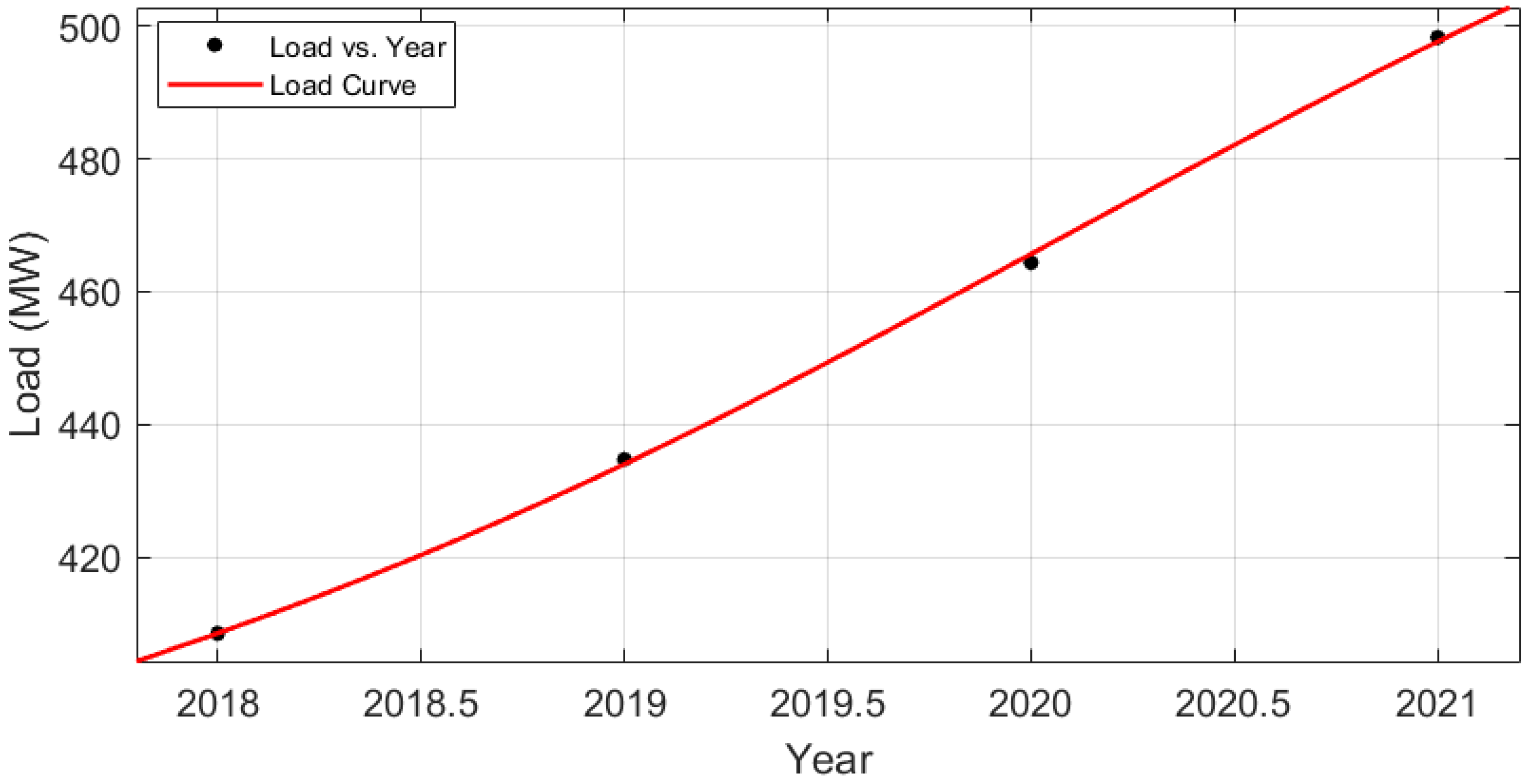
• A linear fit mathematical model is designed for load forecasting corresponding to the projected years, considering the practical data recorded for four consecutive years.
• A study is performed on a part of the RVPN transmission network for the base year (2021) and the projected year (2031).
• A cost–benefit analysis is performed, and it is established that the proposed GOGA provides a financially viable solution with improved flexibility.
• The performance of GOGA is superior compared to a conventional GA-based algorithm.

The paper is arranged into eight sections. Section 1 introduces and discusses reported research related to flexibility and optimization techniques used for optimal placement of REG units in the networks of utility grids. Descriptions of the RVPN transmission network in the Sirohi region considered in the study and the technical parameters are included in Section 2. Load projection for a time horizon of ten years is discussed in Section 3. The proposed GOGA methodology used in the study is described in Section 4. Section 5 details and discusses the simulation results. A cost–benefit analysis is included in Section 6. A comparative performance study of the proposed GOGA and the conventional GA technique is discussed in Section 7. Conclusions are given in Section 8 of the paper.

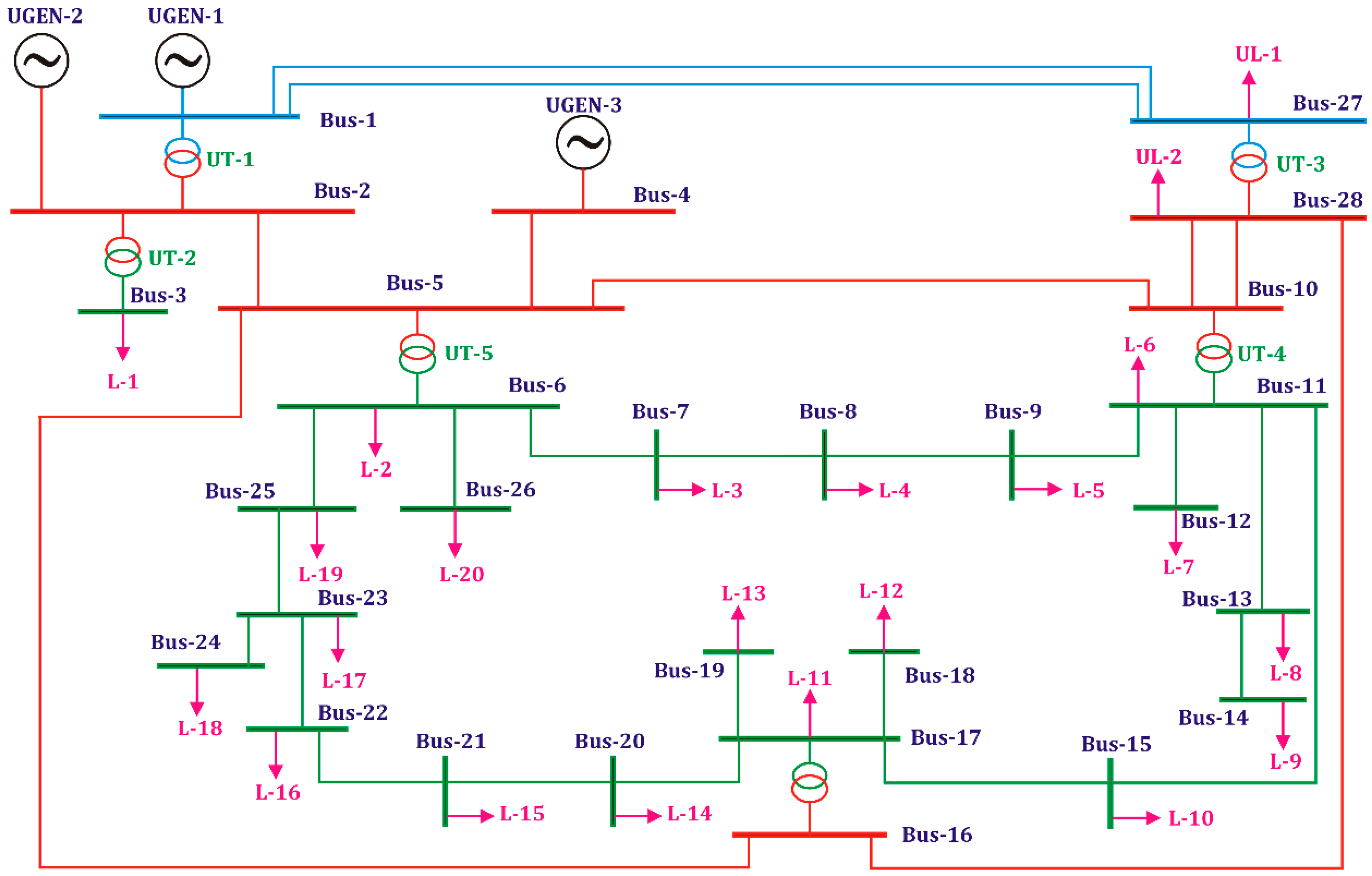
2. Description of Practical Utility Network Used for Study

The RVPN transmission network in the Sirohi region considered in this study is illustrated in Figure 1. RVPN is a State Transmission Utility (STU) in Rajasthan State, India. RVPN plans, designs, builds, maintains, and operates the high-voltage electric transmission system at 132 kV, 220 kV, 400 kV, and 765 kV voltage levels [19]. Details such as total circuit lengths of transmission lines operated at different voltages and the generation and transformer capacities of RVPN are available in [19,20]. The RVPN transmission network considered in the study consists of a total of 28 buses, of which 2 are operated at 400 kV, 6 are operated at 220 kV, and 20 are operated at 132 kV voltage levels. Details of the buses (names and numbers) in the test network and the loads reflected at these buses are provided in

Table 1. Details of buses and base-year loads of test system.

Bus No.	Bus Name	Voltage (kV)	Load Symbol	Peak Load		Average Load		Shunt Reactive Compensation (MVAR)
				P (MW)	Q (MW)	P (MW)	Q (MW)
1	400 kV Barmer	400 kV	-	-	-	-	-	-
2	220 kV Barmer	220 kV	-	-	-	-	-	-
3	132 kV Barmer	132 kV	L-1	-	-	103	29	50
4	220 kV Rajwest	220 kV	-	-	-	-	-	-
5	220 kV Dhaurimanna	220 kV	-	-	-	-	-	-
6	132 kV Dhaurimanna	132 kV	L-2	59.64	15.67	41.748	10.969	10.86
7	132 kV Gudamalani	132 kV	L-3	33.43	10.16	23.401	7.112	10.86
8	132 kV Bagora	132 kV	L-4	59.94	10.9	41.958	7.63	10.86
9	132 kV Jeran	132 kV	L-5	15	7.26	10.5	5.082	5.43
10	220 kV Bhinmal (RVPN)	220 kV	-	-	-	-	-	-
11	132 kV Bhinmal (RVPN)	132 kV	L-6	105.85	33.13	74.095	23.191	16.29
12	132 kV Poonasa	132 kV	L-7	51.56	13.8	36.092	9.66	10.86
13	132 kV Raniwara	132 kV	L-8	35.88	21.32	25.116	14.924	10.86
14	132 kV Sangad	132 kV	L-9	45	26.69	31.5	18.683	10.86
15	132 kV Bhadroona	132 kV	L-10	45.72	11.46	32.004	8.022	10.86
16	220 kV Sanchore	220 kV	-	-	-	-	-	-
17	132 kV Sanchore (220 kV GSS)	132 kV	L-11	8.2	3.97	5.74	2.779	5.43
18	132 kV Sanchore	132 kV	L-12	39.55	13	27.685	9.1	10.86
19	132 kV Paladar	132 kV	L-13	23.83	9.42	16.681	6.594	10.86
20	132 kV Galifa	132 kV	L-14	12.47	1.13	8.729	0.791	5.43
21	132 kV Sata	132 kV	L-15	30.53	12.07	21.371	8.449	10.86
22	132 kV Sedwa	132 kV	L-16	38.66	15.28	27.062	10.696	10.86
23	132 kV Sawa	132 kV	L-17	43.01	21.93	30.107	15.351	10.86
24	132 kV Chohtan	132 kV	L-18	19.5	9.44	13.65	6.608	5.43
25	132 kV Ranasar	132 kV	L-19	29.13	12.41	20.391	8.687	10.86
26	132 kV Ramjiki Gol	132 kV	L-20	15	7.26	10.5	5.082	5.43
27	400 kV Bhinmal (CTU)	400 kV	UL-1	-	-	759	103	150
28	220 kV Bhinmal (CTU)	220 kV	UL-2	-	-	261	22	100

. All loads are considered to be PQ types and are reflected at 132 kV voltage level buses. Loads L1 to L20 indicate the loads supplied to consumers in the region. Actual peak loads recorded on the grid sub-stations (GSSs) were collected. Simultaneous peaking of all the loads was not observed at any of the sub-stations under the actual power operating conditions. Hence, 70% of the peak loads were the values considered in the study to indicate an average load scenario, which was equal to 498.33 MW for the base year of 2021. Furthermore, power export from the study network was equal to 1123 MW, which was mainly handled by the 400 kV D/C transmission line between bus 1 and bus 27. The utility loads UL-1 and UL-2 indicate the power that flows out of the test network through the transmission lines during the average loading scenario.

Details of the generators considered in the study are provided in

Table 2. Generator details.

Bus No.	Symbol of Generator	Voltage (kV)	Pgen (MW)	Qgen (MVAR)
1	UGEN-1	400 kV	1320	264
2	UGEN-2	220 kV	228	44
4	UGEN-3	220 kV	177	35

. These are considered as utility generators (UGEN) and indicate the power that is being fed to the test region. RVPN’s transmission network was created in the MiPower software and simulated using the fast decoupled load flow method. Power flowing to the test network from rest of the network is considered as generation. This power is realized by the utility generators (UGEN-1, UGEN-2, and UGEN-3) in the study. Power flowing out of the test network is represented by the utility loads UL-1 and UL-2. The utility generators used in this study are modelled as thermal power plants because there are lignite-based thermal power plants at Rajwest and Giral that feed power to Sirohi region. Further details of the REGs integrated with the RVPN transmission system in September 2021 are provided in

Table 3. Details of REGs integrated with RVPN transmission system.

Bus No.	Details of REG	Installed Capacity (MW)
1	Solar energy (ground-mounted)	7738
2	Wind energy	4438
3	Biomass	120.38
4	Solar roof-top under net metering scheme	545
Total		12,741.45

. REGs considered for optimal placement in the RVPN transmission system include solar energy, wind energy, and biomass energy [21].

Details of the transmission lines of the test network indicating the emanating and terminating buses, voltage levels, type of conductor, type of circuit (single circuit (S/C) or double circuit (D/C)), and length of the transmission line are included in

Table 4. Details of transmission lines.

Element No.	From Bus No.	To Bus No.	Voltage Level (kV)	Line Length (km)	Type of Conductor	Type of Circuit
1	1	27	400 kV	143.79	Twin Moose	D/C
2	2	5	220 kV	72	ACSR Zebra	S/C
3	4	5	220 kV	90	ACSR Zebra	S/C
4	5	10	220 kV	92.48	ACSR Zebra	S/C
5	5	16	220 kV	64.83	ACSR Zebra	S/C
6	28	10	220 kV	10.37	ACSR Zebra	D/C
7	28	16	220 kV	18.08	ACSR Zebra	S/C
8	6	7	132 kV	67.35	ACSR Panther	S/C
9	7	8	132 kV	32.3	ACSR Panther	S/C
10	8	9	132 kV	21.33	ACSR Panther	S/C
11	9	11	132 kV	21.33	ACSR Panther	S/C
12	11	12	132 kV	26.32	ACSR Panther	S/C
13	11	13	132 kV	51.04	ACSR Panther	S/C
14	13	14	132 kV	26.37	ACSR Panther	S/C
15	11	15	132 kV	22.14	ACSR Panther	S/C
16	15	17	132 kV	51.04	ACSR Panther	S/C
17	17	18	132 kV	35.32	ACSR Panther	S/C
18	17	19	132 kV	6.6	ACSR Panther	S/C
19	17	20	132 kV	18.5	ACSR Panther	S/C
20	20	21	132 kV	50	ACSR Panther	S/C
21	21	22	132 kV	25.4	ACSR Panther	S/C
22	22	23	132 kV	25	ACSR Panther	S/C
23	23	24	132 kV	24	ACSR Panther	S/C
24	24	25	132 kV	19.33	ACSR Panther	S/C
25	25	6	132 kV	21.06	ACSR Panther	S/C
26	6	26	132 kV	25	ACSR Panther	S/C

. There are 27 transmission lines in total, of which 1, 7, and 19 are operated at 400 kV, 220 kV, and 132 kV voltage levels, respectively. Aluminium conductor steel reinforced (ACSR) equivalent Twin Moose, Zebra, and Panther conductors are used on the 400 kV, 220 kV, and 132 kV transmission lines, respectively. Details of these conductors used on the transmission lines are included in

Table 5. Details of transmission-line conductors.

S. No.	Description of Technical Parameters	Numerical Values of Technical Parameter for Various Conductors
		Twin Moose	ACSR Zebra	ACSR Panther
1	Positive sequence resistance	0.0298 Ω/km/circuit	0.0749 Ω/km/circuit	0.1622 Ω/km/circuit
2	Positive sequence reactance	0.332 Ω/km/circuit	0.3992 Ω/km/circuit	0.3861 Ω/km/circuit
3	Positive sequence susceptance (B/2)	1.7344 × 10−6 Ʊ/km/circuit	1.4670 × 10−6 Ʊ/km/circuit	1.4635 × 10−6 Ʊ/km/circuit
4	Zero sequence resistance	0.1619 Ω/km/circuit	0.2200 Ω/km/circuit	0.4056 Ω/km/circuit
5	Zero sequence reactance	1.24 Ω/km/circuit	1.3392 Ω/km/circuit	1.6222 Ω/km/circuit
6	Zero sequence susceptance	1.12 × 10−6 Ʊ/km/circuit	9.2004 × 10−7 Ʊ/km/circuit	1.3171 Ʊ/km/circuit
7	Thermal rating	515 MVA	176 MVA	71 MVA

[22].

Details of transformers installed in the test network, such as interconnecting buses, voltage ratio of transformers, MVA rating of transformers, positive sequence impedance (Z₁), zero sequence impedance (Z₀), ratio of positive sequence reactance (X₁) to positive sequence resistance (R₁), and ratio of zero sequence reactance (X₀) to zero sequence resistance (R₀) are provided in

Table 6. Details of transformers.

From Bus No.	To Bus No.	Voltage Ratio	MVAR Capacity	Transformer Parameters
1	2	400/220 kV	2 × 315 MVA	Z1 = 0.14 pu; (X1/R1) = 20; Z0 = 0.14 pu; (X0/R0) = 20
2	3	220/132 kV	2 × 100 MVA	Z1 = 0.12 pu; (X1/R1) = 20; Z0 = 0.12 pu; (X0/R0) = 20
5	6	220/132 kV	260 MVA	Z1 = 0.12 pu; (X1/R1) = 20; Z0 = 0.12 pu; (X0/R0) = 20
10	11	220/132 kV	2 × 100 MVA	Z1 = 0.12 pu; (X1/R1) = 20; Z0 = 0.12 pu; (X0/R0) = 20
16	17	220/132 kV	100 MVA	Z1 = 0.12 pu; (X1/R1) = 20; Z0 = 0.12 pu; (X0/R0) = 20
27	28	400/220 kV	2 × 315 MVA	Z1 = 0.14 pu; (X1/R1) = 20; Z0 = 0.14 pu; (X0/R0) = 20

.

3. Load Projection

The maximum loads recorded for the test network during four consecutive years are provided in

Table 7. Maximum loads recorded in the test network during the last four financial years.

S. No.	Particulars	Year
		2018	2019	2020	2021
1	Recorded maximum load (MW)	408.47	434.69	464.38	498.33
2	Rate of annual load growth (%)	-	6.42%	6.83%	7.31%

. It can be observed that load was continuously increasing and the rate of annual load growth (RALG) was also increasing. The recorded maximum loads and the RALG were used to forecast the load for next ten-year time horizon (up to the year 2031) using the least-square approximation method. The curve-fitting tool of the MATLAB software was used to find the best-fitting linear model using the least-square approximation technique to forecast the load. A load versus year fitted load curve is plotted in Figure 2. A detailed description of the least-square approximation method is available in [23,24]. The linear fit mathematical model used to compute the projected load (PL) is described by Equation (1), and was used for load projections up to the year 2031.

$$PL\left(x\right)=a\times \left(sin\left(x-\pi \right)\right)+b\times \left({\left(x-10\right)}^2\right)+c$$

(1)

where, x is the year for which the load is computed, a is 7.783, b is 0.006296, and c is −2.497 × 10⁴. The coefficients a, b, and c are computed with 95% confidence bounds. The sum of squared estimates of errors (SSE) was equal to 2.58 and the root mean square error (RMSE) was 1.606. R-squared was equal to 0.9994. Values of R-squared nearly equal to unity indicate the perfect prediction capability of the proposed model. Lower values of the RMSE and SSE indicate a better fit of the data. Hence, the model proposed in Equation (1) will provide a load projection for the test system corresponding to the years up to 2031. The projected loads of the test network for a 10-year time horizon computed using Equation (1) are provided in

Table 8. Projected loads of test network for 10-year time horizon.

Particulars	Year
	2022	2023	2024	2025	2026	2027	2028	2029	2030	2031
Projected Load (MW)	524.335	543.89	562.15	585.62	616.05	648.80	677.09	698.29	716.26	737.86

. Further, the reflection of the projected loads at individual load buses of the test network corresponding to the projected year 2031 are shown in

Table 9. Details of projected loads on network buses corresponding to projected year 2031.

Bus No.	Bus Name	Voltage (kV)	Load Symbol	Average Load
				P (MW)	Q (MW)
3	132 kV Barmer	132 kV	L-1	103	29
6	132 kV Dhaurimanna	132 kV	L-2	61.81482	16.24142
7	132 kV Gudamalani	132 kV	L-3	34.64905	10.53049
8	132 kV Bagora	132 kV	L-4	62.12576	11.29748
9	132 kV Jeran	132 kV	L-5	15.54699	7.524742
11	132 kV Bhinmal (RVPN)	132 kV	L-6	109.7099	34.33811
12	132 kV Poonasa	132 kV	L-7	53.44018	14.30323
13	132 kV Raniwara	132 kV	L-8	37.18839	22.09745
14	132 kV Sangad	132 kV	L-9	46.64096	27.66327
15	132 kV Bhadroona	132 kV	L-10	47.38722	11.8779
17	132 kV Sanchore (220 kV GSS)	132 kV	L-11	8.49902	4.114769
18	132 kV Sanchore	132 kV	L-12	40.99222	13.47406
19	132 kV Paladar	132 kV	L-13	24.69898	9.763508
20	132 kV Galifa	132 kV	L-14	12.92473	1.171206
21	132 kV Sata	132 kV	L-15	31.6433	12.51014
22	132 kV Sedwa	132 kV	L-16	40.06977	15.8372
23	132 kV Sawa	132 kV	L-17	44.57839	22.72969
24	132 kV Chohtan	132 kV	L-18	20.21108	9.784237
25	132 kV Ranasar	132 kV	L-19	30.19225	12.86254
26	132 kV Ramjiki Gol	132 kV	L-20	15.54699	7.524742
27	400 kV Bhinmal (CTU)	400 kV	UL-1	759	103
28	220 kV Bhinmal (CTU)	220 kV	UL-2	261	22

.

4. Proposed Method

The proposed methodology used for the study is illustrated in Figure 3. A part of the RVPN transmission system in the Sirohi region of India was considered in the study as a test network. Furthermore, technical data for all transmission lines, transformers, and generation sources for this test network were collected. For the years 2018, 2019, 2020, and 2021, the recorded peak loads on all the grid sub-stations (GSS) of the test network were collected. Projections of the loads were computed for the next 10 years using the methodology detailed in Section 3. The test network was modelled in MATLAB software and simulated without renewable energy generators (REGs) for the base year (2021) and the projected year (2031) using the Newton–Raphson load flow technique to compute power flows in transmission elements, voltage profiles at all test network buses, system losses, and losses in all transmission lines. Optimal sizing and placement of the REGs using the proposed grid-oriented genetic algorithm (GOGA) is described in the following sub-sections. Furthermore, the proposed approach can also be used effectively for standard test systems such as the IEEE 39-bus system and the New England 68-bus system because the RVPN transmission system is a practical utility network and has more issues/constraints than standard test systems such as the IEEE 39-bus system and the New England 68-bus system, in terms of loading of lines, voltage variations, system stability, power system protection, power quality, etc. Hence, the proposed GOGA will work effectively on standard test systems also.

4.1. Formulation of Objective Function

Optimal sizing and placement of REGs using the GOGA was achieved with the objective of loss minimization. Active power losses (P_L) in the test network are expressed as a function of the power generated by different units and expressed using the Kron equation [25], as detailed below.

$$P_L={\displaystyle {{\displaystyle \sum }}_{i=1}^{ng}}{\displaystyle {{\displaystyle \sum }}_{i=1}^{ng}}{b}_{ij}{P}_i{P}_j+{\displaystyle {{\displaystyle \sum }}_{i=1}^{ng}}{b}_{i0}{P}_i+b_{00}$$

(2)

A simplified form of the above equation is detailed below, which is used by the grid-oriented genetic algorithm (GOGA) for loss computation.

$$P_L=P_g^{T}B{P}_g+P_g^T{B}_0+B_{00}$$

(3)

Here, B = [b_ij], B₀ = [b_i0], B₀₀ = [b₀₀], and P_g^T = [p₁ p₂… p_ng]. In addition, n_g is the number of REG units, and P_i and P_j are the active power values generated at the ith and jth buses, respectively. The matrices B, B₀, and B₀₀ are loss coefficients and are computed by adopting the method described in [25]. These coefficients are dependent on the system loads and generation.

4.2. Optimal Sizing of REGs

To determine the optimal sizing and location of REG units, it is assumed that n_g REG units are installed on buses k_n1, k_n2, …, k_ng. Further, it is also assumed that all REG units are operating at a power factor of unity. Bus 1 of the test system is considered as a slack bus, and two conventional generators are also considered in the test system. Hence, there are ng + 3 generation units in the test network. Further, it is also assumed that the REG units are installed on buses 5, 6, …, N. Here, N is the total number of buses in the test system, which is equal to 28 in this study. Because conventional generators are installed on buses 1, 2, and 4, buses 1–4 are exempted from the installation of REG units. Network losses are at a minimum when the derivative of the expression for P_L with respect to P_i is zero. P5 to P28 are considered as the power generated by the REG units on buses 5 to N, respectively. This generated power is independent of the power generated by the slack bus and the conventional generation units. The sum of the system losses (P_L) and the total system demand (P_D) is equal to the power generated by the slack bus, conventional generators, and REG units, as detailed below, where the network demand (P_D) is assumed to be constant.

$$P_L+P_D=P_1+P_2+P_4+{\displaystyle {{\displaystyle \sum }}_{j=5}^N}{P}_j$$

(4)

Differentiating Equation (4) yields

$$\frac{\partial P_L}{\partial P_i}+\frac{\partial P_D}{\partial P_i}=\frac{\partial P_1}{\partial P_i}+\frac{\partial P_2}{\partial P_i}+\frac{\partial P_4}{\partial P_i}+{\displaystyle {{\displaystyle \sum }}_{j=5}^N}\frac{\partial P_j}{\partial P_i}$$

(5)

At the optimum solution point, the partial derivative of the constant terms is zero. The power generated by the slack bus (P₁) is dependent on the power generated by the different REG units. For the condition of minimum system losses, the ratio of active power changes generated by the slack bus to those generated by the REG units is equal to −1. This is achieved when the last term of Equation (5) is zero, because here the condition of j = i will be satisfied and the partial derivative will be equal to 1. For this condition, the terms for network loss and total demand $\partial P_L/\partial P_i$ and $\partial P_D/\partial P_i$ in Equation (5) will be zero. Further, the power generated by the REGs is at a maximum at the optimal solution point, which ensures that the terms $P_1/\partial P_i,$ $\partial P_2/\partial P_i$, and $\partial P_4/\partial P_i$ are also zero. Hence, at the optimal solution point, Equation (5) will take the form shown below.

$$\frac{\partial P_1}{\partial P_i}=-1$$

(6)

The condition specified by Equation (6) will give the optimum solution with the highest generation from the REGs and the minimum network loss. To minimize Equation (2), provided that the condition of Equation (6) is satisfied, the Lagrangian relaxation method as described in [25] was used to find the optimal sizing of the REG units. In the RVPN transmission system, generators are operated at near-unity power factors. Reactive power exchange between the utility network and the generator is kept to minimum, and active power is exchange is kept to a maximum at the point of grid integration of generators. Hence, reactive power is not considered in the above equations. Furthermore, reactive compensation in the RVPN transmission system is achieved using the shunt capacitor banks and the reactor at the GSS to maintain the voltage profile. This also keeps the reactive power flow in the transmission lines to a minimum and the active power flow to a maximum.

4.3. GOGA for Optimal Allocation of REG Units

A grid-oriented genetic algorithm (GOGA) was applied to determine the optimal locations of the REG units for minimum system losses. A genetic algorithm (GA) is an optimization method and is used to solve different optimization problems. The GA proceeds in several steps, as described in [26]. In this study, two grid parameter variables were considered in an optimization problem for each REG unit in the GA, which is considered to be a GOGA. These variables were the active power generated by the REG units and the location of the REG unit on a particular bus of the test network. The active power of the REG unit was computed using the mathematical formulation described in Section 4.2. In the GOGA, the location of REG units is considered a problem of variable chromosomes. Hence, considering the number of REG units, the length of the chromosomes will be ng, considering ng genes for the location of REG units (R5, R6, …, RN). The GOGA is implemented in the following steps:

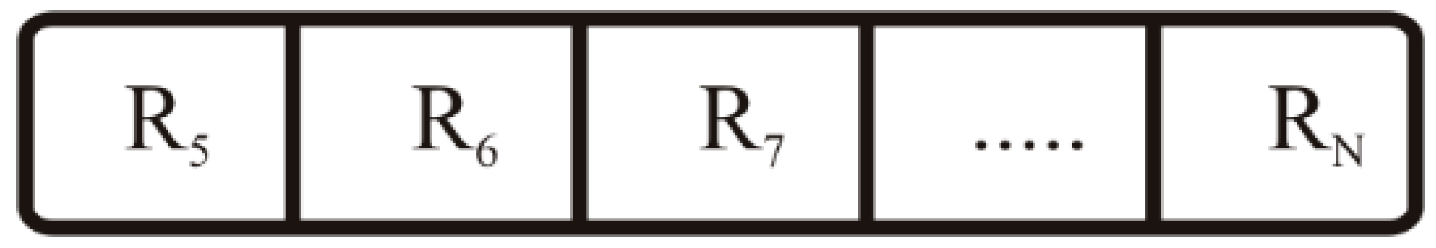
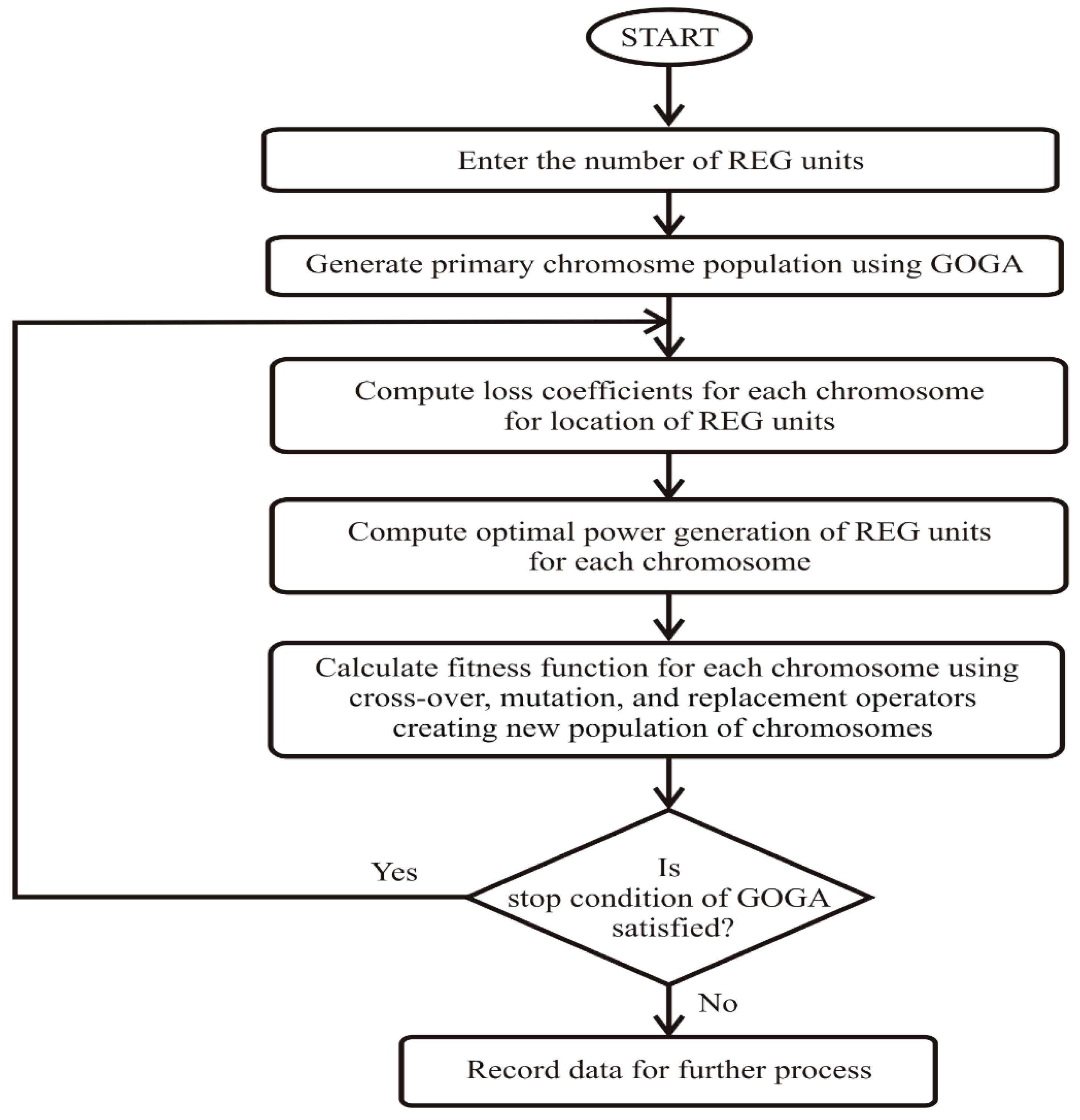
• A set of chromosomes is randomly produced, which indicates the possible solutions for REG location. The form of the chromosomes considered in the study is shown in Figure 4.
• A number is allocated to every chromosome with respect to its fitness, to find a possible solution. This indicates the number determined by the fitness function, which will be optimized by the GOGA.
• To compute the fitness function corresponding to a chromosome, the network loss is computed using Equation (3), and the optimal power generation of the REG units computed in Section 4.2 is considered.
• A power flow run is performed, and the system losses are computed using Equation (2) and assigned to a chromosome as a fitness value. The GOGA searches for the lowest value of the fitness function by changing the location of the REG units. The lower boundary of the fitness function is zero, and an upper boundary is not required because the objective is to reduce the loss. However, the actual system losses without placement of REG units are considered as the upper-boundary values. These losses were 62.185 MW and 139.224 MW for the base year without REG placement, in the base year (2021) and the projected year (2031).

  $$fitness=P_{loss}$$

  (7)
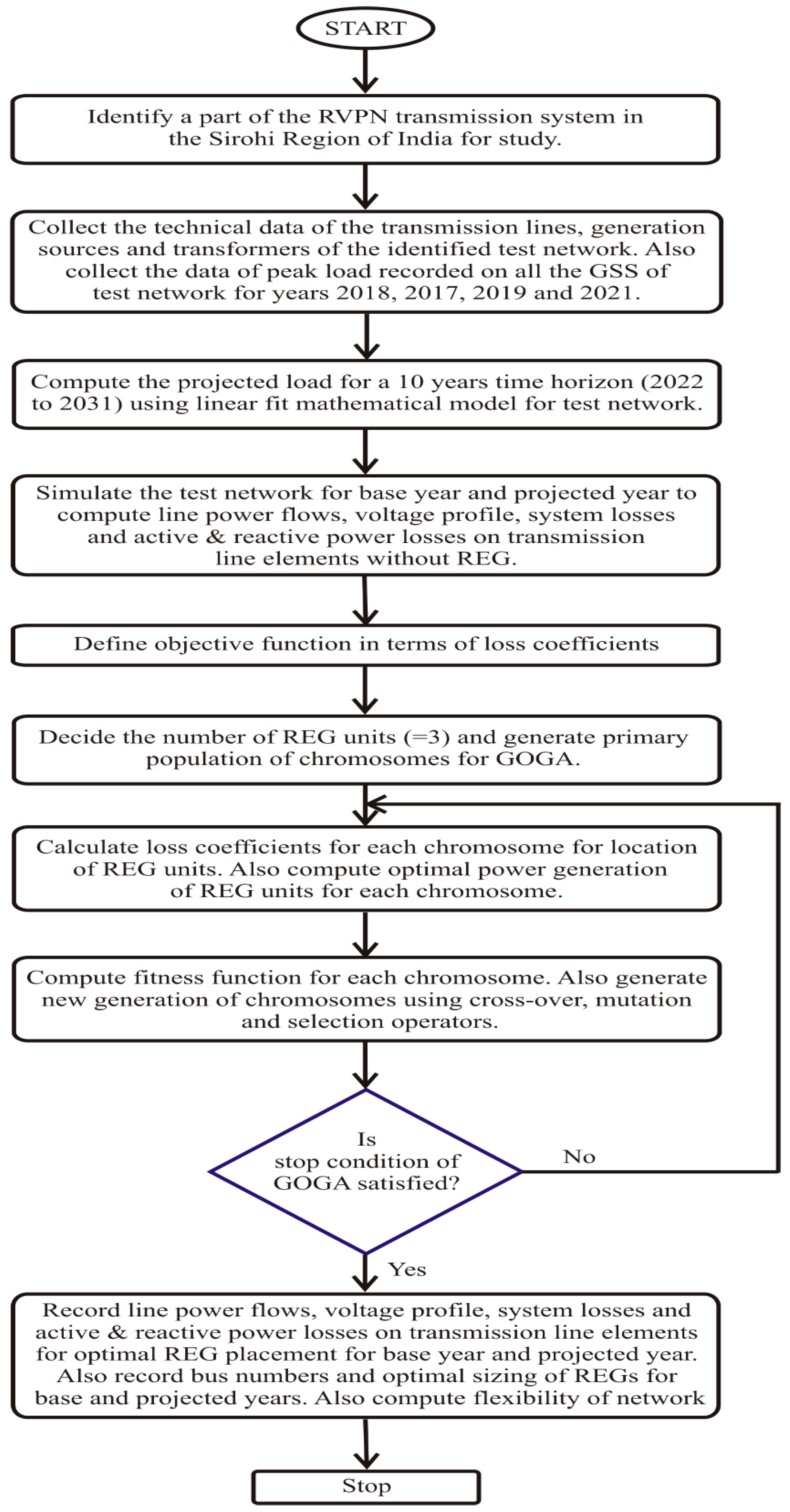
• The GOGA selects some chromosomes for crossover, mutation, and replacement operators using selection operators, with respect to the fitness of the chromosomes. These operators generate a new chromosome, and the process is repeated until the stop condition is satisfied. A schematic diagram of the GOGA optimization approach for optimal placement and sizing of REG units is depicted in Figure 5.

4.4. Computation of Flexibility

A flexibility index (FI) is proposed to assess the flexibility of the test network for supplying quality power to consumers. It is based on deviations of the voltages at all buses in the test network and the total system losses of the test network. The FI is computed using the following expression:

$$FI=\left(\frac{1}{\frac{\Delta V}{V}+\frac{P_L}{P_G}}\right)\times 100$$

(8)

where ΔV indicates the sum of the voltage deviations at each bus of the test network and P_G is the sum of the power generated by all the generators and REG units in the test system. For the purpose of calculating voltage deviations, the nominal voltage at each bus is considered to be unity. Higher values of the FI indicate higher flexibility, and lower values of the FI indicate low flexibility of the test network for meeting consumer demand.

5. Simulation Results and Discussion

Results were obtained for the base year (2021) and projected year (2031) without renewable energy generators (REGs) and considering the optimal placement of REGs using the proposed GOGA. The Newton (NR) method was used for load flow analysis for all four conditions. The convergence characteristic of the GOGA for optimal placement of REGs for the conditions corresponding to the base year is illustrated in Figure 6. It can be observed that optimal REG placement results were achieved in 42 iterations, indicating fast convergence. Similarly, the convergence characteristic of the GOGA for optimal placement of REGs for conditions corresponding to the projected year is illustrated in Figure 7. It can be observed that optimal REG placement results were achieved in 26 iterations, indicating fast convergence.

Table 10. Optimal sizes of REGs for base year and projected year.

Bus No.	Optimal Size of REGs Using GOGA		Proposed REG Capacity
	Base Year	Projected Year
6	150 MW	120 MW	150 MW
14	0	22 MW	25 MW
22	15 MW	6 MW	15 MW

shows the sizes of the REGs and the corresponding number of placements computed using the GOGA, for the base year and the projected year. After considering the scenarios of the base year and the projected year, the sizes of the REGs were also suggested for installation in the test network, as shown in Table 10. If the proposed REGs were installed in the recent scenario, then network expansion would not be required for the next 10 years.

The profiles of the voltages recorded on all the network buses for the base year and the projected year without REGs and with optimal placement of the REGs using the GOGA is illustrated in Figure 8. It can be observed that for conditions corresponding to the base year, the voltages on all buses were maintained within the permissible limits. However, optimal placement of the REGs using the GOGA further improved the voltage profile. For the projected year, voltages decreased drastically, violating the voltage limits. This was due to increased bus loads and overloading on the transmission lines and transformers. Optimal placement of the REGs on buses 6, 14, and 32 improved the voltage profiles on all buses for the projected year 2031, and the voltages on all buses were within the permissible limits.

Power flows in all the transmission line elements of the test network for the conditions corresponding to the base year and the projected year are included in

Table 11. Power flows in transmission lines and transformers for base year and projected year.

From Bus No.	To Bus No.	Line Power Flows for Year 2021				Line Power Flows for Year 2031
		Without REG		With REG		Without REG		With REG
		MW	MVAR	MW	MVAR	MW	MVAR	MW	MVAR
17	19	16.727	−13.131	18.137	2.126	24.807	−7.085	23.468	6.185
1	27	1068.068	56.464	1060.089	125.235	1206.448	318.476	1190.243	182.079
2	5	331.545	−57.869	338.539	−33.514	502.469	148.01	443.225	50.554
4	5	177	−45.963	187.837	−24.555	177	112.376	179.272	40.714
5	10	126.932	−14.563	145.557	4.647	140.364	60.281	136.305	26.018
5	16	152.326	−41.896	168.398	−8.240	190.496	41.847	176.604	24.903
28	10	52.475	−50.422	39.834	6.652	148.982	−52.598	131.174	30.530
28	16	−24.331	−32.163	−32.261	−9.328	1.356	−50.231	2.535	−5.130
6	7	74.59	−38.933	84.472	−15.796	105.798	−1.994	96.740	1.793
7	8	49.416	21.346	57.281	−8.701	67.099	1.914	60.195	1.543
8	9	6.973	−7.363	11.967	−4.632	3.799	6.905	2.483	−1.700
9	11	−3.537	4.838	0.688	3.658	−11.787	12.714	−11.636	1.333
11	12	36.686	−2.554	37.586	9.082	55.532	6.646	47.936	14.993
11	13	57.573	−12.043	59.045	16.402	87.475	20.476	75.396	36.605
13	14	31.697	−3.566	31.734	13.376	47.432	11.579	39.515	22.737
11	15	2.186	−14.261	2.064	−5.535	9.232	−17.734	9.959	−5.436
15	17	−29.892	−8.758	−32.349	0.529	−38.403	−17.44	−33.953	−8.086
17	18	27.728	−5.431	30.041	7.240	41.122	0.29	39.009	12.039
17	20	43.467	−31.551	45.400	−4.038	69.237	−15.041	63.737	9.854
20	21	34.343	−17.389	34.324	1.933	55.24	−5.977	52.269	12.288
21	22	12.382	−12.27	12.051	1.711	21.749	−6.158	20.141	7.114
22	23	−14.718	2.095	−16.260	4.819	−18.368	−2.164	−14.739	1.475
23	24	−44.889	11.483	−47.922	3.379	−63.169	−5.143	−54.304	−9.755
24	25	−59.015	22.638	−63.226	9.373	−84.613	−3.406	−74.648	−9.473
25	6	−80.104	33.997	−86.176	13.424	−116.514	−1.896	−106.331	−11.072
6	26	10.515	−12.781	11.555	−1.452	15.582	−7.303	15.294	2.014
2	3	104.073	11.983	93.430	21.210	104.073	11.983	93.430	21.210
1	2	210.447	11.564	181.776	11.540	388.526	74.409	295.626	40.583
5	6	213.755	−104.504	73.239	−142.534	314.952	1.893	162.296	−61.111
27	28	294.95	18.391	281.078	33.947	427.75	212.486	385.793	122.513
10	11	177.315	−42.104	48.061	−51.903	285.193	9.928	159.791	159.791
16	17	125.688	−65.138	−2.954	−88.519	187.278	−17.198	66.596	−38.742

. It can be observed that optimal placement of REGs of optimal sizes helps to reduce loading on the critically overloaded transmission elements for both the base-year scenario and the projected-year scenario. Loading on all transmission lines is within permissible limits, even for the next 10 years.

5.1. Losses in the Network

The active power losses on the individual transmission line elements for the base year and the projected year without REGs, which are considered as distributed generators (DG), and with optimal placement of REGs using the GOGA are illustrated in Figure 9. It can be observed that line losses for the conditions corresponding to the base year were small. Similarly, these losses were reduced slightly after the optimal placement of the REGs on buses 6, 14, and 22 for the base-year scenario. Further, it can be observed that for the projected year, losses in individual transmission line elements increased significantly due to overloading of these transmission elements. The optimal placement of the REGs on buses 6, 14, and 22 for the projected-year scenario significantly reduced the transmission line losses.

The reactive power losses in individual transmission line elements for the base year and the projected year without the REGs and with optimal placement of the REGs using the GOGA are illustrated in Figure 10. It can be observed that the reactive power line losses for the conditions corresponding to the base year were small. Similarly, these losses were reduced slightly after the optimal placement of the REGs on buses 6, 14, and 22 for the base-year scenario. Further, it can be observed that for the projected year, losses in individual transmission line elements increased significantly due to overloading of these transmission elements. The optimal placement of the REGs on buses 6, 14, and 22 for the projected-year scenario significantly reduced the transmission line losses.

The total system losses for the test network corresponding to the base year and the projected year are provided in

Table 12. Network losses and loss savings due to optimal placement of REG units.

Bus No.	Particulars	Network Losses
		Without REG Placement		With Optimal REG Units Placement
		2021	2031	2021	2031
1	Active power loss (MW)	62.185	139.224	55.733	86.894
2	Loss saving due to optimal REG placement (MW)	--		6.452	52.33

. It can be observed that the system losses increased from 62.185 MW in the base year to 139.224 MW in the projected year. The losses in the base year were reduced from 62.185 MW (3.83%) to 55.733 MW (3.44%) after optimal placement of the REGs at buses 6, 14, and 22. Similarly, for the projected year, the losses were reduced from 139.224 MW (7.48%) to 86.894 MW (4.67%) after optimal placement of the REGs at buses 6, 14, and 22. Hence, it is established that optimal placement of the REGs helps to reduce the system losses significantly, simultaneously reducing overloading of the transmission elements.

5.2. Computation of Flexibility

A flexibility index (FI) was computed to evaluate the flexibility of the test network to feed power to consumers for the base year and the projected year, considering the scenarios with and without REG units. The magnitudes of the flexibility index for the base year without REG units (FI2021), the flexibility index for the base year with REG units (FI2021REG), the flexibility index for the projected year without REG units (FI2031), and the flexibility index for the projected year with REG units (FI2031REG) computed using Equation (8) are included in

Table 13. Details of flexibility index.

Flexibility Index	Magnitude of FI
FI2021	74.84
FI2021REG	99.01
FI2031	30.94
FI2031REG	78.81

. It can be observed that the network is more flexible for supplying power to the consumers with optimal placement of the REG units during the base year, because the flexibility index (FI) increased from 74.84 without REG units to 99.01 in the presence of REG units. The flexibility of the network decreased drastically during the projected year compared to the base year, as indicated by the magnitude of the FI, which was 74.84 in the base year and 30.94 in the projected year. Optimal placement of the REG units during the projected year improved the flexibility significantly, to a value better than that of the base year without REG units. The FI magnitude in the projected year increased from 30.94 without REG units to 78.81 with REG units. Hence, the optimal placement of REG units improved the flexibility of the test network for feeding power to the consumers.

6. Cost–Benefit Analysis

A cost–benefit analysis was carried out to compute the payback period for the installation costs of the REG units. The electricity tariff in Indian rupees (INR) was INR 7.65/kWh [27]. The total cost for the installation of a renewable energy generator with a capacity of 10 kW, including wiring charges, operation costs, and maintenance costs, was INR 82,000 [28]. The total loss saving for the base year due to the REG units was equal to 6.452 MW, as detailed in Table 11. Hence, the total annual cost savings due to the placement of REG units during the base year (CS2021) is described by the following expression.

$$CS2021=\left(6.452\mathrm{MW}\right)\times 1000\times \left(\frac{\mathrm{INR}7.65}{\mathrm{kWh}}\right)\times 8760=\mathrm{432,374,328}\frac{\mathrm{INR}}{\mathrm{year}}$$

(9)

The total investment cost for the placement of REG units (CREG2021) of capacity 165 MW is computed by the following expression.

$$CREG2021=\frac{\mathrm{82,000}\times 190\times 1000}{10}=\mathrm{1,558,000,000}\frac{\mathrm{INR}}{\mathrm{year}}$$

(10)

The payback period (PBP) is expressed as the ratio of capital cost to the total saving cost and is computed using the following expression [29].

$$BP=\frac{\mathrm{1,558,000,000}}{\mathrm{432,347,328}}=3.603\mathrm{year}$$

(11)

The cost of installation of the REG units will be recovered over a time period of 3.603 years if installation is considered to be in the base year. Similarly, if installation is considered to be in the projected year, then the payback period is only 0.37 years. Hence, it is recommended that installation of REG units should be considered in the base year to obtain maximum benefit.

7. Performance Comparison Study

The performance of the proposed GOGA was compared with the results of the GA reported in [30] by applying both approaches to the RVPN transmission system considered in this study. The total capacity of the REG units using the GA was computed to be equal to 230 MW in the base year, compared to 55.733 MW using the GOGA. Furthermore, the loss saving using the GA algorithm was found to be equal to 4.321 MW, whereas the loss saving using the GOGA was 6.452 MW. Accordingly, the payback period using the GA was found to be 6.513 years for the base year, compared to 3.603 years using the GOGA. Hence, the GOGA gives a more optimal solution compared to the GA for placement and sizing of REG units in the RVPN transmission system for loss minimization and flexibility improvement.

8. Conclusions

This paper presented a detailed study of a practical transmission network and proposed a grid-oriented genetic algorithm for optimal placement of REG units to improve the power system flexibility. The GOGA was based on a hybrid combination of a genetic algorithm and solutions using analytical power flow equations for optimal sizing and placement of REG units. Power system network loss minimization, reduced voltage deviations, and flexibility improvements were achieved on a part of the practical transmission network of RVPN in the Sirohi region of India for the base year (2021) and the projected year (2031). A linear fit mathematical model was effectively used to forecast the load of the test network for a 10-year time horizon. It was established that the GOGA provides a financially viable solution with improved flexibility through optimal placement of REG units. The voltages on all buses in the test network were recorded as within permissible limits after optimal placement and sizing of the REG units. It was also established that the GOGA ensures high convergence speed and good solution accuracy. Loss savings of 6.452 MW and 52.33 MW were achieved for the base year and the projected year, respectively, via optimal REG placement. The payback period for the base year was 3.603 years, and for the projected year it was 0.37 years. Hence, it is concluded that installation of REG units will be more beneficial if considered in the base year. Furthermore, the performance of the GOGA was superior in terms of loss reduction via optimal sizing and placement of REG units compared to a conventional GA.

References

1. Abudu, K.; Igie, U.; Roumeliotis, I.; Hamilton, R. Impact of gas turbine flexibility improvements on combined cycle gas turbine performance. Appl. Therm. Eng. 2021, 189, 116703. [Google Scholar] [CrossRef]
2. Yang, B.; Wang, J.; Chen, Y.; Li, D.; Zeng, C.; Chen, Y.; Guo, Z.; Shu, H.; Zhang, X.; Yu, T.; et al. Optimal sizing and placement of energy storage system in power grids: A state-of-the-art one-stop handbook. J. Energy Storage 2020, 32, 101814. [Google Scholar] [CrossRef]
3. Abdelaziz, A.Y.; Hegazy, Y.G.; El-Khattam, W.; Othman, M.M. A Multiobjective Optimization for Sizing and Placement of Voltage Controlled Distributed Generation Using Supervised Big Bang Big Crunch Method. Electr. Power Compon. Syst. J. 2015, 43, 105–117. [Google Scholar] [CrossRef]
4. Othman, M.M.; Hegazy, Y.G.; Abdelaziz, A.Y. Electrical Energy Management in Unbalanced Distribution Networks using Virtual Power Plant Concept. Electr. Power Syst. Res. 2017, 145, 157–165. [Google Scholar] [CrossRef]
5. Shaheen, A.M.; Elsayed, A.M.; El-Sehiemy, R.A.; Abdelaziz, A.Y. Equilibrium Optimization Algorithm for Network Reconfiguration and Distributed Generation Allocation in Power Systems. Appl. Soft Comput. J. 2021, 98, 106867. [Google Scholar] [CrossRef]
6. Lannoye, E.; Flynn, D.; O’Malley, M. Evaluation of Power System Flexibility. IEEE Trans. Power Syst. 2012, 27, 922–931. [Google Scholar] [CrossRef]
7. Zongo, O.A.; Oonsivilai, A. Optimal placement of distributed generator for power loss minimization and voltage stability improvement. Energy Procedia 2017, 138, 134–139. [Google Scholar] [CrossRef]
8. Lannoye, E.; Flynn, D.; O’Malley, M. Transmission, Variable Generation, and Power System Flexibility. IEEE Trans. Power Syst. 2015, 30, 57–66. [Google Scholar] [CrossRef]
9. Shrimali, G. Managing power system flexibility in India via coal plants. Energy Policy 2021, 150, 112061. [Google Scholar] [CrossRef]
10. Das, C.K.; Bass, O.; Kothapalli, G.; Mahmoud, T.S.; Habibi, D. Optimal placement of distributed energy storage systems in distribution networks using artificial bee colony algorithm. Appl. Energy 2018, 232, 212–228. [Google Scholar] [CrossRef]
11. Zhao, H.; Jiang, P.; Chen, Z.; Ezeh, C.I.; Hong, Y.; Guo, Y.; Zheng, C.; Džapo, H.; Gao, X.; Wu, T. Improvement of fuel sources and energy products flexibility in coal power plants via energy-cyber-physical-systems approach. Appl. Energy 2019, 254, 113554. [Google Scholar] [CrossRef]
12. Maeder, M.; Weiss, O.; Boulouchos, K. Assessing the need for flexibility technologies in decarbonized power systems: A new model applied to Central Europe. Appl. Energy 2021, 282, 116050. [Google Scholar] [CrossRef]
13. Kopiske, J.; Spieker, S.; Tsatsaronis, G. Value of power plant flexibility in power systems with high shares of variable renewables: A scenario outlook for Germany 2035. Energy 2017, 137, 823–833. [Google Scholar] [CrossRef]
14. Guo, Z.; Zheng, Y.; Li, G. Power system flexibility quantitative evaluation based on improved universal generating function method: A case study of Zhangjiakou. Energy 2020, 205, 117963. [Google Scholar] [CrossRef]
15. Chen, J.; Qi, B.; Rong, Z.; Peng, K.; Zhao, Y.; Zhang, X. Multi-energy coordinated microgrid scheduling with integrated demand response for flexibility improvement. Energy 2021, 217, 119387. [Google Scholar] [CrossRef]
16. Feng, J.; Yang, J.; Wang, H.; Wang, K.; Ji, H.; Yuan, J.; Ma, Y. Flexible optimal scheduling of power system based on renewable energy and electric vehicles. In Proceedings of the 2021 8th International Conference on Power and Energy Systems Engineering (CPESE 2021), Fukuoka, Japan, 10–12 September 2021. [Google Scholar]
17. Xu, J.; Ma, Y.; Li, K.; Li, Z. Unit commitment of power system with large-scale wind power considering multi time scale flexibility contribution of demand response. In Proceedings of the 2021 International Conference on Energy Engineering and Power Systems (EEPS2021), Hangzhou, China, 20–22 August 2021. [Google Scholar]
18. Zhang, H.; Shen, J.; Wang, G. Day-ahead stochastic optimal dispatch of LCC-HVDC interconnected power system considering flexibility improvement measures of sending system. Int. J. Electr. Power Energy Syst. 2022, 138, 107937. [Google Scholar] [CrossRef]
19. RVPN. Rajasthan Rajya Vidyut Prasaran Nigam Limited. 2021. Available online: https://energy.rajasthan.gov.in/content/raj/energy-department/rajasthan-rajya-vidyut-prasaran-limited/en/home.html## (accessed on 20 November 2021).
20. Ola, S.R.; Saraswat, A.; Goyal, S.K.; Jhajharia, S.; Rathore, B.; Mahela, O.P. Wigner distribution function and alienation coefficient-based transmission line protection scheme. IET Gener. Transm. Distrib. 2020, 14, 1842–1853. [Google Scholar] [CrossRef]
21. Rajasthan Renewable Energy Corporation. Available online: https://energy.rajasthan.gov.in/content/raj/energy-department/rrecl/en/home.html# (accessed on 26 February 2022).
22. CEA. Central Electricity Authority. Transmission Planning Criteria. 2021. Available online: https://cea.nic.in/transmission-planning-criteria/?lang=en (accessed on 20 November 2021).
23. Axelsson, O. A generalized conjugate gradient, least square method. Numer. Math. 1987, 51, 209–227. [Google Scholar] [CrossRef]
24. Chen, G.; Ren, Z.L.; Sun, H.Z. Curve fitting in least-square method and its realization with Matlab. Ordnance Ind. Autom. 2005, 3, 063. [Google Scholar]
25. Stevenson, W., Jr.; Grainger, J. Power System Analysis; McGraw-Hill Education: New York, NY, USA, 1994. [Google Scholar]
26. Vatani, M.; Alkaran, D.S.; Sanjari, M.J.; Gharehpetian, G.B. Multiple distributed generation units allocation in distribution network for loss reduction based on a combination of analytical and genetic algorithm methods. IET Gener. Transm. Distrib. 2016, 10, 66–72. [Google Scholar] [CrossRef]
27. RERC. Tariff for Supply of Electricity-2020; Rajasthan Electricity Regulatory Commission: Jaipur, India, 2021. Available online: https://energy.rajasthan.gov.in/content/raj/energydepartment/en/departments/jvvnl/Tariff_orders.html (accessed on 20 November 2021).
28. Solar Panel Installation Cost in India. Loom Solar, India. 2021. Available online: https://www.loomsolar.com/blogs/collections/solar-panel-installation-cost-in-india (accessed on 20 November 2021).
29. Agajie, T.F.; Khan, B.; Alhelou, H.H.; Mahela, O.P. Optimal expansion planning of distribution system using grid-based multi-objective harmony search algorithm. Comput. Electr. Eng. 2020, 87, 106823. [Google Scholar] [CrossRef]
30. Gopu, P.; Naaz, S.; Aiman, K. Optimal Placement of Distributed Generation using Genetic Algorithm. In Proceedings of the 2021 International Conference on Advances in Electrical, Computing, Communication and Sustainable Technologies (ICAECT), Bhilai, India, 19–20 February 2021. [Google Scholar] [CrossRef]
Figure 1. Test transmission network of Sirohi region, India.
Energies 15 01863 g001
Figure 2. Curve of recorded load for test network during four consecutive years.
Energies 15 01863 g002
Figure 3. Proposed methodology of study using GOGA.
Energies 15 01863 g003
Figure 4. Form of chromosome.
Energies 15 01863 g004
Figure 5. Schematic diagram of GOGA optimization approach for optimal placement and sizing of REG units.
Energies 15 01863 g005
Figure 6. Convergence characteristic of GOGA for optimal REGs placement for condition corresponding to base year.
Energies 15 01863 g006
Figure 7. Convergence characteristic of GOGA for optimal REGs placement for condition corresponding to projected year.
Energies 15 01863 g007
Figure 8. Voltage profile on network buses for base year and projected year without REGs and with optimal placement of REGs.
Energies 15 01863 g008
Figure 9. Active power losses in transmission line elements for base year and projected year.
Energies 15 01863 g009
Figure 10. Reactive power losses in transmission line elements for base year and projected year.
Energies 15 01863 g010