A Dynamic Simulation Model for a Heat Exchanger Malfunction Monitoring

Abstract

Modelling and simulation is presented for a finned cross-flow heat exchanger with the aim to heat cold air to be fed to air conditioning batteries for marine purposes. The model employed in this paper is finalized to simulate the dynamic behavior of air and water temperatures fed to the air conditioning batteries operating in cold environments, in order to predict possible troubles owing to the change in input parameters, such as unwanted flow rate variations due to system malfunctions. In the investigated model, heat balance equations are presented and discretized by Laplace transform, which has the advantage to easily account for the different structures of heaters used for the purpose of validation. The model was implemented in the Matlab-Simulink environment for its high capacity of dealing with dynamic systems. The results of the model are satisfactory, as the dynamic behavior of the air stream temperature is correctly reproduced, as compared to experimental data, providing a suitable parameter for malfunctions prediction.

1. Introduction

Heat exchangers can be applied to many purposes [1,2,3], among which is the heating of an air current for the most disparate scopes. This paper presents the model of a heat exchanger to be applied to heat cold air in air conditioning batteries operating in cold environments. The heat exchanger to be modeled in this paper is a cross-flow air–water unit, equipped with fins in the air side, where a flow of hot water passes into a pipe invested by the current of air to be heated. The unit is employed for marine purposes.

The main interest of this article is the implementation of a dynamic simulation model to predict air and water temperature behavior in different dynamic conditions, in order to detect malfunctions of the system. In fact, the operation in cold environments may produce, in particularly cold conditions, malfunctions such as the freezing of water in some sections of the heat exchanger, causing its blocking. Therefore, the model employed needs to reproduce the dynamics of the main parameters to changing conditions, such as, for example, the feed-water flow rate or its inlet temperature.

Laplace transforms are quite a popular tool and are well suited in the considered problem to the modelling of two dimensional heat exchangers using a simple one-dimensional model.

In the present paper, a technique based on the solution of heat balance equations was employed by relying on the discretizing of such equations and using Laplace transform. Laplace transforms allow to easily account for the different structures of heaters, which have been used for the purpose of validation. The heat exchanger employed in the experiments is a cross-flow unit, and a discretization operated with the Laplace transform is able to take into account the bi-dimensional extension of the heat exchanger, as it can sub-divide it into “ranks”, each one representing one layer of the coils, as explained in the following sections.

In literature, several models for representing heat exchangers behavior are reported, since the argument is very interesting for many applications and accurate modelling is important for control, maintenance, and safety purpose. The articles reported in literature include simple models in which each stream exchanging heat is modelled as a series of mixed tanks [4]; such simulation scheme can also be able to represent the dynamic behavior of the system. The model has been employed to discriminate the more important and less important features by order of magnitude argumentation.

More complex approaches employ the distributed parameters method as in [5], which presents a comprehensive and detailed model for both the evaporator and condenser of refrigerant cycles. It has been shown in literature that the so-called “tube-by-tube approach” [6] tends to provide a more accurate and realistic prediction in terms of the interfacial structure for both the evaporator and the condenser. The tube-by-tube method allows to predict the heat exchanger duty such as air temperature and relative humidity for each tube. The local data are displayed for the tubes, identifying the tube connection, which makes a detailed analysis of the conditions that affect the duty of the evaporator and of the condenser easier.

Other models are employed for reproducing different configurations of heat exchangers [7]; such models are developed in algorithmic form for steady-state simulation. The configuration is defined by the number of channels, number of passes in each side, fluid locations, feed connection locations, and type of channel-flow with the purposes of studying the configuration influence on the heat exchanger performance and to further develop a method for configuration optimization.

Ordinary differential equations are used too for the purpose of modelling heat exchangers [8]. Generally, the thermal circuit models result in sets of ordinary differential equations which are numerically solved. The system of equations derived from the traditional thermal resistance capacity model are usually stiff and make results unstable, unless employing a very small time step, which significantly increases the run time. Instead, the system of ordinary differential equations described in the cited model is non-stiff and there is no time step limitation for the stability of the results.

The finite volume method is proposed in [9], where it is applied for the thermal performance prediction of a hybrid earth to air tunnel heat exchanger. Process parameters are optimized using response surface methodology by the use of a commercial Computational Fluid Dynamics (CFD) based software to simulate the heat exchanger, the turbulence model, and to carry out a two-dimensional simulation modelling. Moreover, response surface methodology is applied to analyze the results of finite volume method and to optimize the process parameters of the hybrid earth to the air tunnel heat exchanger. Other models employing CFD can be found in [10,11,12,13].

Another modelling technique is the moving boundary method [14]. In particular, the cited article employs a more accurate moving boundary method that incorporates analytic enthalpy distributions. The enthalpy profiles are derived by defining a specific heat capacity at each thermodynamic phase of a binary mixture and by solving crossflow heat transfer equations.

In literature can also be found a comparison between finite volume methods and moving boundary methods [15] useful when the governing dynamics of the system are mainly concentrated in the heat exchangers, as in small Organic Rankine Cycles investigated. The modeling of the system is characterized by evaporation or condensation. This requires heat exchanger models capable of handling phase transitions. As a consequence, the accuracy and simulation speed of the higher level system model mainly depend on the heat exchanger model formulation and the finite volume and the moving boundary approaches are the most widely used.

Models based on partial differential equations can be found, which can use either analytical or numerical approaches [16,17]. In [16], the temperature transient response of a single-phase fluid and a wall in a heat exchanger is analyzed, in order to reproduce the behavior of the system when the other constant temperature fluid is subjected to a step change in temperature or when the single-phase fluid is subjected to a step change in mass flow rate. To reproduce the dynamic behavior of the heat exchanger, an approximation is used by an integral method, hypothesizing that the single-phase fluid temperature distribution can be expressed by a combination of the initial and final temperature distributions and a time function. In [17], an innovative coil dynamic model is presented that utilizes the exact solution to the coil governing partial differential equation for a step change in water flow rate.

The analytical solutions of equations describing the dynamics of distributed parameter systems are usually complicated and difficult to use for the purpose of simulation and control system design. In [18], an analytical solution of the dynamics of a symmetrically operated counter flow heat exchanger in the form of transfer function matrix is investigated in open-loop and close-loop conditions.

Data-based techniques, also known as black box models, can also be found [19]. The complexity of a mathematical model is critical when the model needs to be employed for deriving the control law, as it directly affects the complexity of the mathematical transformations and of the control algorithm. In paper [19], the simplified cross convection model for a wide class of heat exchangers is suggested. The main frame of this model is derived from energy conservation and combined with simple dynamics based on ordinary differential equations. By this method, the simplified tuning procedure of the proposed model is suggested and verified for plate and spiral tube heat exchangers based on experimental data.

Finally, artificial neural networks can be employed for the modelling of heat exchangers. In [20], the potentials of neural networks-based control techniques are investigated by applying a nonlinear generalized minimum variance control methodology to a simulated application example. In particular, the paper faces the problem of regulating the output temperature of a liquid-saturated steam heat exchanger by adjusting the liquid flow-rate. Owing to the non-minimum phase characteristic of the process dynamics, a simple inverting minimum variance controller results unsuitable. However, an effective solution is provided by the introduction of a penalization factor in the control variable. A steady-state off-set error problem, caused by the neural network approximations, is faced by the use of a hybrid control structure, which combines a nonlinear integral action block with a neural controller. In [21], the artificial neural network technique is applied to the simulation of the time-dependent behavior of a heat exchanger in order to control the temperature of air, also providing experiments carried out in an open loop test facility. First, a methodology is proposed for the training and prediction of thermal systems’ dynamic behavior with heat exchangers. Then, an internal model scheme is developed for the control of the over-tube air temperature with two artificial neural networks, one to simulate the heat exchanger and the other employed for the controller. An integral control is implemented in parallel with the filter of the neural network controller to eliminate the steady-state offset.

The paper is organized as follows: in Section 2, the modelling technique is presented, introducing the main control variables, the effect of the fins by introducing correction factors to the classical equations, the dynamic equations to be solved, and the method of their discretization over the space, paying particular attention to the Laplace transform methodology; in Section 3 is first provided a calibration of the model parameters based on the data measured on the plant, and then the simulation of a dynamic situation characterized by a shut-down of the hot water inlet valve is described, presenting the diagrams of water, copper tube, and air temperatures in function of time for measured and simulated variables, changing the number of discretization elements. In addition, an error analysis is carried out. Finally, the conclusions are drawn.

2. Modelling Technique

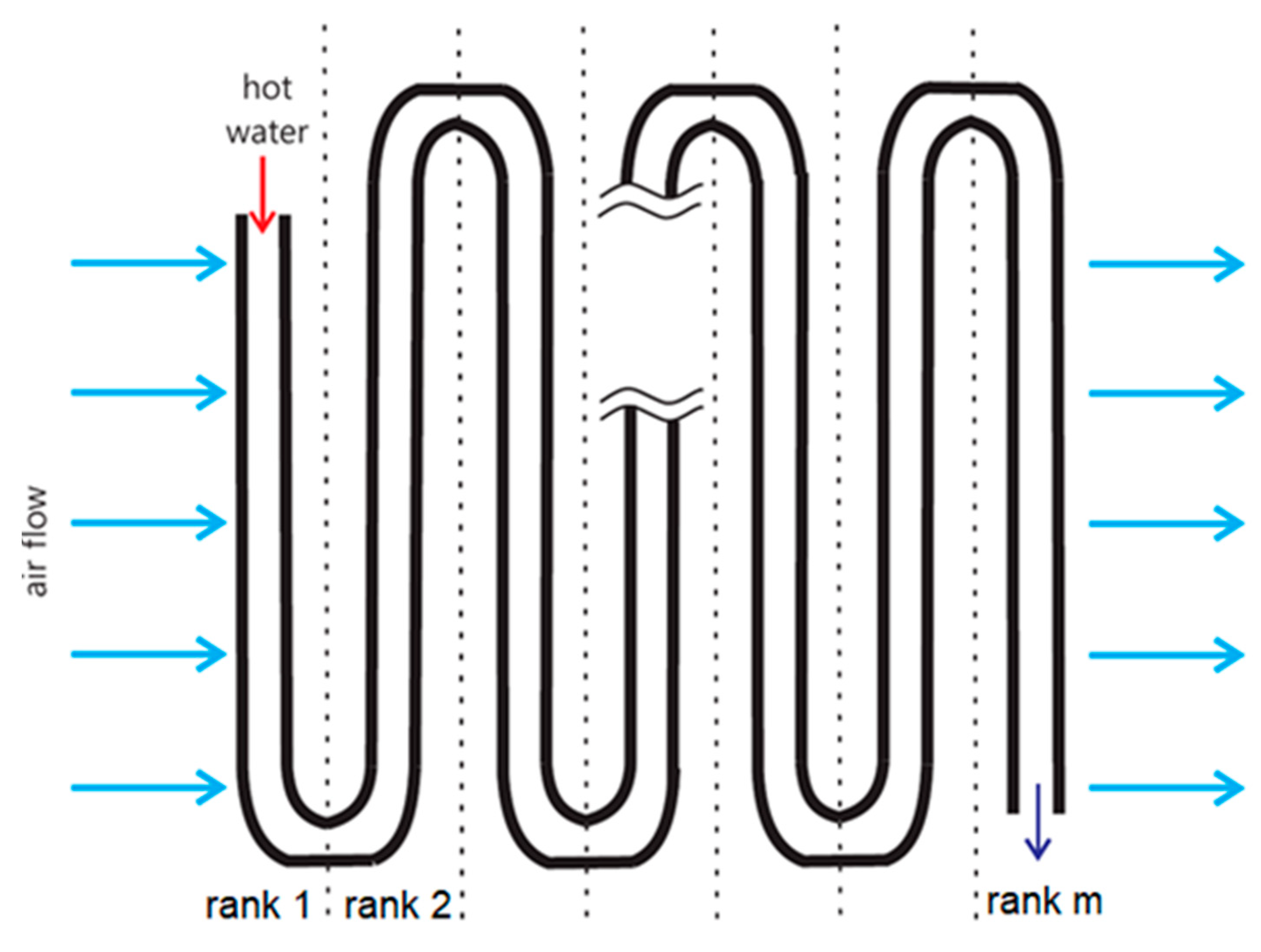
The model of a heat exchanger battery is constructed by applying the heat balance equations that result from the flow of hot water in the coils, which are finned in the air side. In practice, the model will be developed for each coil composing the battery. The coils are spread over m layers, as shown in Figure 1, each of which will be denoted by the name “rank” in the following. Each of the ranks receives a flow of air from the previous one.

The air entering the battery is heated by passing from one rank to the next one, owing to the heat exchange from the hot water flowing in the tube (made of copper) and from the finned tube to the air. For the purpose of the heat exchanger, which is to provide heating to the air conditioning batteries, the water leaving the coil is at a lower temperature as compared to the entrance temperature.

To model the thermodynamics of such coil system, it is necessary to make the following assumptions:

(1)

thermal dispersion towards the environment is assumed to be zero;

(2)

upstream and downstream temperature of the air in each rank is assumed to be uniform;

(3)

upstream and downstream temperature of the coil in each rank is assumed to be uniform;

(4)

the temperature of the hot water and the coil at the coil entrance are assumed to be equal.

The response time of a lumped capacity system increases with its total capacitance (also known as thermal mass), and decreases with its surface area, and with the overall heat transfer coefficient. In the present case, estimations of the capacitance and surface area are possible and depend also on the total surface area of the heat exchange surface and on its geometry.

To proceed, it is required to introduce a suitable set of parameters and variables as follows.

• Inlet air: h₁ is the air heat transfer coefficient, r₁ is the air density, C₁ is the air specific heat capacity, W₁ is the air flow rate, and T₁ is the air temperature.
• Inlet hot water: h₂ is the water heat transfer coefficient, r₂ is the water density, C₂ its specific heat capacity, W₂ is the water flow rate, and T₂ is the water temperature.
• Tube wall: r₃ is the copper density, C₃ its specific heat capacity and T₃ is the temperature, considered uniform within the pipe thickness.
• L is the length of the coil.
• A₁ and A₂ are the outer and inner areas of the tube, respectively.
• S₁ is the perimeter of the outer part of the copper tube, while S₂ the perimeter of the inner part of the tube.

Figure 2 illustrates the main variables required to construct the model, as explained above. The quantity dx represents the elementary length of the pipe.

2.1. Effect of the Fins

Concerning the model for the effect of the fins crossing the tube in the air side, in general the heat exchange occurring between an air flow and a smooth tube provides a thermal flow $q$, whose value is given by the formula in Equation (1):

$$q=h{A}_{smooth}\left(T_{tube}-T_{air}\right)$$

(1)

where $h$ is the heat transfer coefficient of the tube in air, $A_{smooth}$ is the surface of the tube, $T_{tube}$ is the temperature of the tube, and $T_{air}$ is the temperature of the air. If the tube is finned, this equation must be modified, taking into account the surface efficiency ${\eta }_0$, as in Equation (2):

$$q={\eta }_{0}h{A}_{finned}\left(T_{tube}-T_{air}\right)$$

(2)

where $A_{finned}$ can be obtained from the geometric properties of the tube and of the fins. In practice, it is useful to define a fin factor $F$ as in Equation (3):

$$F=\frac{A_{finned}}{A_{smooth}}$$

(3)

and thus it is possible to proceed by replacing $A_{smooth}$ with ${\eta }_{0}F{A}_{finned}$.

2.2. Balance Dynamic Equations

The dynamic equations of a battery can be obtained by using three thermal balances:

(1)

heat balance of the inlet air

(2)

heat balance of the inlet hot water

(3)

heat balance of the wall of the coil.

Such balance equations have to be computed contemporaneously to attain a lumped parameter model well-suited to being simulated.

The heat balance for air is based on the first law of thermodynamics, which remarks the conservation of the enthalpy and takes into account the exchange of heat with the tube, as in Equation (4):

$$W_1{C}_1{T}_1+{\eta }_{0}F{h}_1{S}_{1}dx\left(T_3-T_1\right)-\left(W_1{C}_1{T}_1+W_1{C}_1\frac{d{T}_1}{dx}dx\right)=r_1{A}_{1}dx{C}_1\frac{d{T}_1}{dt}$$

(4)

where $W_1{C}_1{T}_1$ is the heat flow entering with the inlet water, ${\eta }_{0}F{h}_1{S}_{1}dx\left(T_3-T_1\right)$ is the heat flow exchanged with the coil, $W_1{C}_1{T}_1+W_1{C}_1\frac{d{T}_1}{dx}dx$ the output heat flow and $r_1{A}_{1}dx{C}_1\frac{d{T}_1}{dt}$ the variation of the heat accumulated in the air.

Similarly, the heat balance equation for the inlet hot water exchanging heat with the wall of the tube is obtained, as shown in Equation (5):

$$W_2{C}_2{T}_2+h_2{S}_{2}dx\left(T_3-T_2\right)-\left(W_2{C}_2{T}_2+W_2{C}_2\frac{d{T}_2}{dx}dx\right)=r_2{A}_{2}dx{C}_2\frac{d{T}_2}{dt}$$

(5)

where $W_2{C}_2{T}_2$ is the input heat flow, $h_2{S}_{2}dx\left(T_3-T_2\right)$ is the heat flow exchanged between the water and the tube, $W_2{C}_2{T}_2+W_2{C}_2\frac{d{T}_2}{dx}dx$ the output heat flow of the water, and $r_2{A}_{2}dx{C}_2\frac{d{T}_2}{dt}$ the variation of the heat accumulated in the water.

Finally, the thermal balance of the copper tube is provided in Equation (6):

$${\eta }_{0}F{h}_1{S}_{1}dx\left(T_1-T_3\right)+h_2{S}_{2}dx\left(\overline{T_2}-T_3\right)=r_3{A}_{3}dx{C}_3\frac{d{T}_3}{dt}$$

(6)

where ${\eta }_{0}F{h}_1{S}_{1}dx\left(T_1-T_3\right)$ is the heat flow leaving the tube towards the air, $h_2{S}_{2}dx\left(\overline{T_2}-T_3\right)$ the heat flow entering in the tube from the water; $r_3{A}_{3}dx{C}_3\frac{d{T}_3}{dt}$ the variation of the heat accumulated in the copper tube. $A_3=A_1-A_2$, whereas ${\overline{T}}_2$ is the average temperature of the hot water in the considered rank.

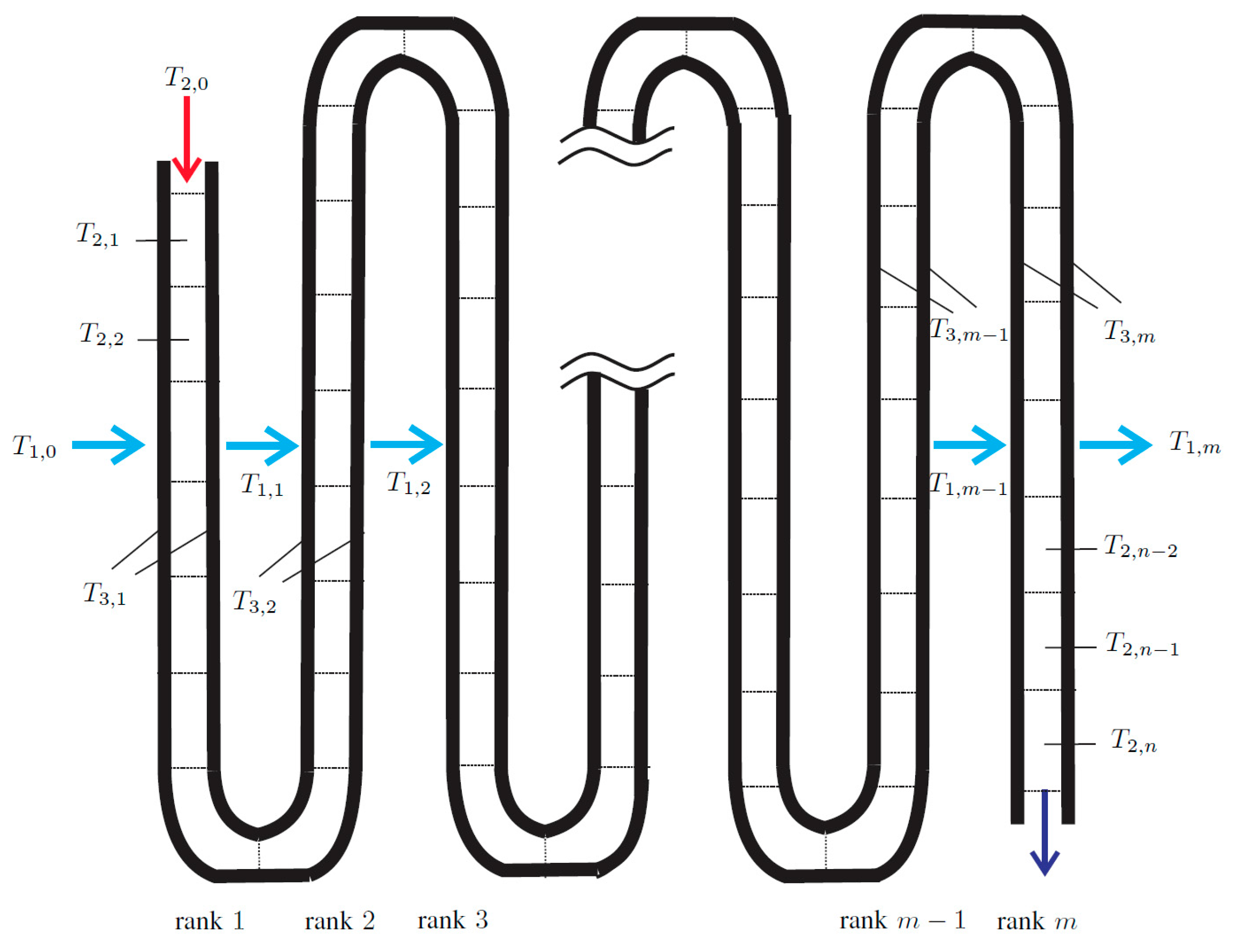
2.3. Discretization over the Space

The three enthalpy balance equations need to be discretized over space for being treated numerically. The coils are divided into n sections. Thus, the following quantities are defined (see Figure 3):

• the temperature of the hot water in section i is denoted by T_2,i
• T_1,i is the temperature of the air upstream inlet flow at rank j + 1.
• T_1,j+1 is the temperature of the air downstream inlet flow at rank j + 1.
• T_3,k is the temperature of the tube at rank k.

Based on the aforesaid, it is possible to discretize and derive the corresponding Laplace representation in the complex domain s ∈ C.

From rank m, by discretizing all the heat balance equations, for the wall of the coil Equation (7) is obtained:

$${\eta }_{0}F{h}_1{S}_1\delta x\left(T_{1,m}-T_{3,m}\right)+h_2{S}_2\delta x\left({\overline{T}}_{2,m}-T_{3,m}\right)=r_3{A}_3\delta x{C}_3\frac{d{T}_{3,m}}{dt}$$

(7)

where $\delta x=L/n_m$ is space sample step and $n_m$ is the number of sections in rank $m$ and the temperature variable ${\overline{T}}_{2,m}$ is the average temperature over the rank m, calculated as in Equation (8):

$${\overline{T}}_{2,m}=\frac{1}{n_m}{\displaystyle \sum }_{i=0}^{n_m-1}{T}_{2,m-i}$$

(8)

Hence, after the application of Laplace transform, the resulting terms appear in Equation (9):

$$(r_3{A}_3{C}_{3}s+{\eta }_{0}F{h}_1{S}_1+h_2{S}_2)T_{3,m}\left(s\right)={\eta }_{0}F{h}_1{S}_1{T}_{1,m}\left(s\right)+h_2{S}_2{\overline{T}}_{2,m}\left(s\right)$$

(9)

where, from now on, $T_{3,m}\left(s\right)$ denotes the Laplace transform of $T_{3,m}\left(t\right)$ and similarly for the other state variables. Thus, expressing the equation in a more compact form, it is possible to write Equation (10):

$$T_{3,m}\left(s\right)=\frac{{\alpha }_3}{{\tau }_{3}s+1}{T}_{1,m}\left(s\right)+\frac{{\beta }_3}{{\tau }_{3}s+1}{\overline{T}}_{2,m}\left(s\right)$$

(10)

where the Greek symbols are listed in Equation (11) below as:

$${\tau }_3=\frac{r_3{C}_3{A}_3}{{\eta }_{0}F{h}_1{S}_1+h_2{S}_2}; {\alpha }_3=\frac{{\eta }_{0}F{h}_1{S}_1}{{\eta }_{0}F{h}_1{S}_1+h_2{S}_2}; {\beta }_3=\frac{h_2{S}_2}{{\eta }_{0}F{h}_1{S}_1+h_2{S}_2}$$

(11)

As the inlet air flow is valid, the discretized energy balance is as reported in Equation (12):

$${\eta }_{0}F{h}_1{S}_1\delta x\left(T_{3,m}-T_{1,m}\right)-W_1{C}_1\left(T_{1,m}-T_{1,m-1}\right)=r_1{A}_1\delta x{C}_1\frac{d{T}_{1,m}}{dt}$$

(12)

Hence, by applying the Laplace transform, the mathematical representation reported in Equation (13) appears:

$$(r_1{A}_1{C}_1\delta x s+{\eta }_{0}F{h}_1{S}_1\delta x+W_1{C}_1)T_{1,m}\left(s\right)=W_1{C}_1{T}_{1,m-1}\left(s\right)+{\eta }_{0}F{h}_1{S}_1\delta x{T}_{3,m}\left(s\right)$$

(13)

which can also been written, in compact form, as in Equation (14):

$$T_{1,m}\left(s\right)=\frac{{\alpha }_1}{{\tau }_{1}s+1}{T}_{1,m-1}\left(s\right)+\frac{{\beta }_1}{{\tau }_{1}s+1}{T}_{3,m}\left(s\right)$$

(14)

where the Greek symbols meanings are reported in Equation (15) below as:

$${\tau }_1=\frac{r_1{C}_1{A}_1\delta x}{{\eta }_{0}F{h}_1{S}_1\delta x+W_1{C}_1}; {\alpha }_1=\frac{W_1{C}_1}{{\eta }_{0}F{h}_1{S}_1\delta x+W_1{C}_1}; {\beta }_3=\frac{{\eta }_{0}F{h}_1{S}_1\delta x}{{\eta }_{0}F{h}_1{S}_1\delta x+W_1{C}_1}$$

(15)

Equation (16) expresses the thermal balance equation for the inlet water:

$$h_2{S}_2\delta \overline{x}\left(T_{3,m}-T_{2,n-1}\right)-W_2{C}_2\left(T_{2,n}-T_{2,n-1}\right)=r_2{A}_2\delta \overline{x}{C}_2{\frac{d{T}_{2,n}}{dt}}_{}$$

(16)

where $\delta \overline{x}=L/n$, n being the space step samples in which the water pipe has been subdivided. Therefore, by the application of the Laplace transform, the terms in Equation (17) appear:

$$(r_2{A}_2{C}_2\delta \overline{x} s+h_2{S}_2\delta x+W_2{C}_2)T_{2,n}\left(s\right)=W_2{C}_2{T}_{2,n-1}\left(s\right)+h_2{S}_2\delta \overline{x}{T}_{3,m}{\left(s\right)}_{}$$

(17)

and finally, in compact form:

$$T_{2,n}\left(s\right)=\frac{{\alpha }_2}{{\tau }_{2}s+1}{T}_{2,n-1}\left(s\right)+\frac{{\beta }_2}{{\tau }_{2}s+1}{T}_{3,m}\left(s\right)$$

(18)

where the Greek symbols appearing in Equation (18) are defined in Equation (19) below:

$${\tau }_2=\frac{r_2{C}_2{A}_2\delta \overline{x}}{h_2{S}_2\delta \overline{x}+W_2{C}_2}; {\alpha }_2=\frac{W_2{C}_2}{h_2{S}_2\delta \overline{x}+W_2{C}_2}; {\beta }_2=\frac{h_2{S}_2\delta \overline{x}}{h_2{S}_2\delta \overline{x}+W_2{C}_2}$$

(19)

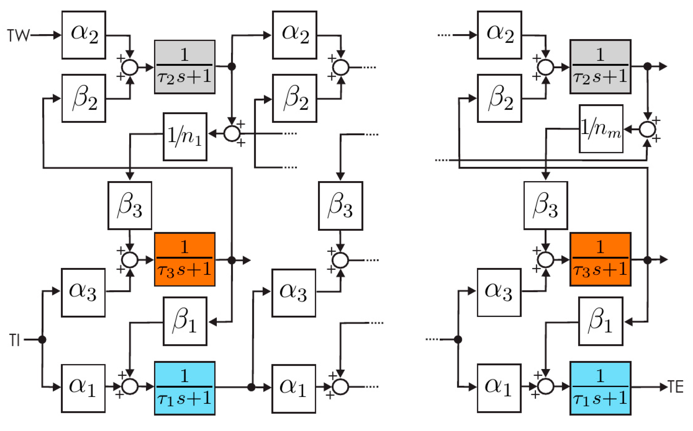
The resulting block diagram, implemented in a Matlab-Simulink environment, is depicted in Figure 4.

Figure 4 represents the “core” of the model, while the complete implementation scheme for the heat exchanger simulation model is depicted in Figure 5.

In Figure 5, it is possible to observe the Simulink blocks by which the whole model of the heat exchanger is composed, for a heat exchanger equipped with three ranks. In the picture, it is possible to observe:

• The fault generator, where the water flow reduction simulating the failure is introduced; this block is constituted by a Simulink switch, by which it is possible to select the faulty-non faulty modality. The faulty modality operates as described in the following Section 2.4, by influencing the parameter α₂ of the water.
• The ranks sequence, in which water, air, and copper temperature are computed rank by rank; in the picture, three ranks are represented. In particular, for each rank, the “Water Temperature”, “Copper Temperature”, and “Air Temperature” blocks contain the Laplace equations dedicated to calculating the corresponding temperatures. Such equations are, respectively, Equations (10), (14) and (18).

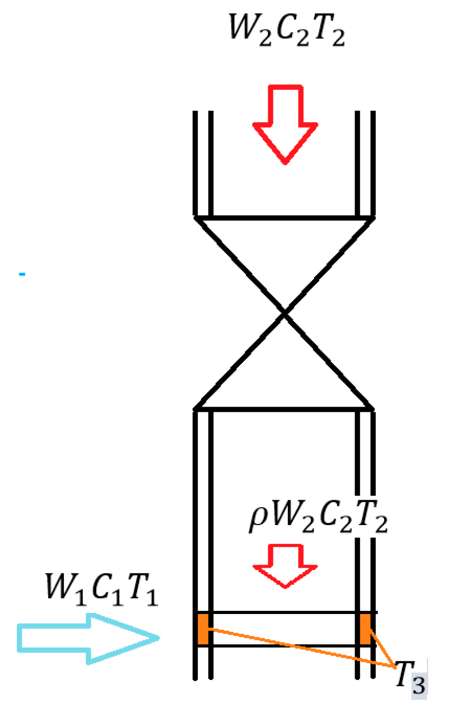
2.4. Accounting for Water Flow Reduction

In principle, the nine system parameters ${\tau }_1$, ${\alpha }_1$, ${\beta }_1$, ${\tau }_2$, ${\alpha }_2$, ${\beta }_2$, ${\tau }_3$, ${\alpha }_3$, ${\beta }_3$, can be derived by using standard physical constants according to their definitions, but in practice they need to be tuned.

If the flow of inlet hot water reduces, the heat exchange between the water and the tube wall and therefore between the tube wall and air, drops. In practice, as pictorially shown in Figure 6, it is possible to account for this effect by reducing the initial flow rate from $W_2$ to a fraction of this value, i.e., $\rho W_2$, where $\rho$ is a number comprised 0 and 1. The decrease of $W_2$ of a factor $\rho$ causes a change in the parameter ${\alpha }_2$.

3. Results

3.1. Calibration of the Model

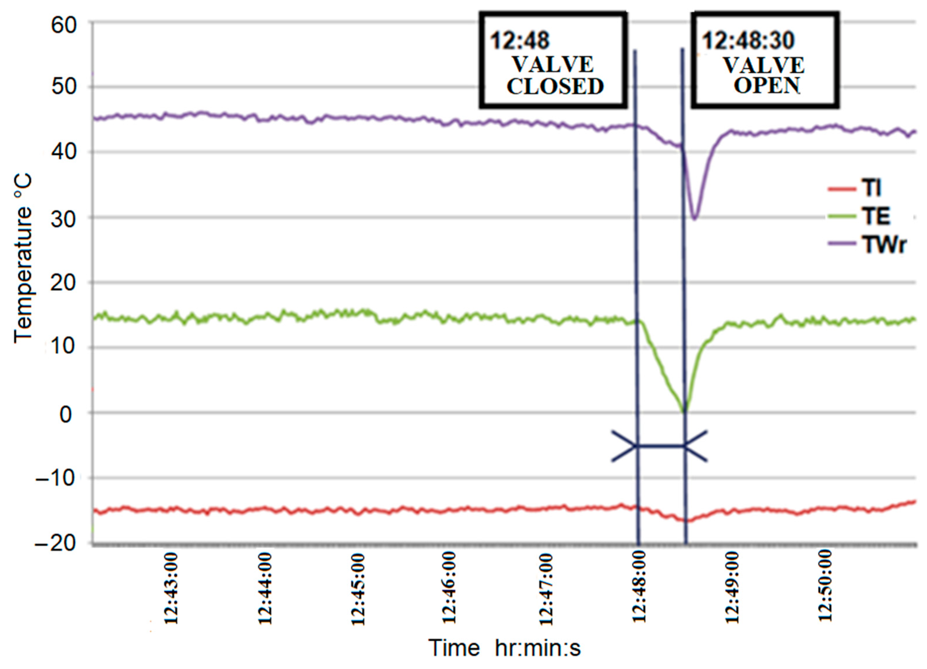
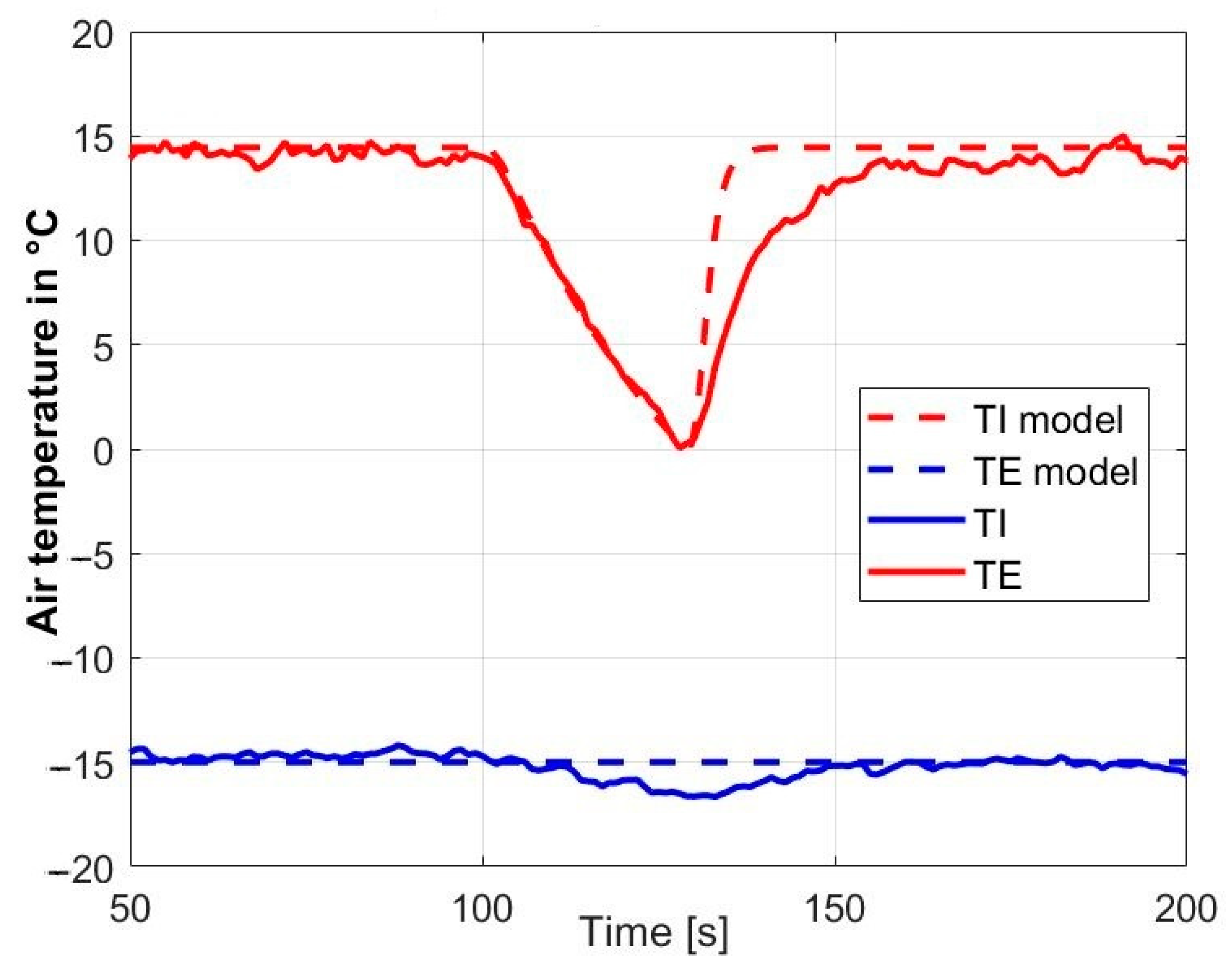
Based on the model depicted in Figure 4, the nine system parameters ${\tau }_1$, ${\alpha }_1$, ${\beta }_1$ for the air flow, ${\tau }_2, {\alpha }_2, {\beta }_2$ to account for the water dynamics and ${\tau }_3, {\alpha }_3, {\beta }_3$ to account for copper pipe dynamics were calibrated by using the records of a test for a particular geometric configuration of the heat exchanger, employing the data at regime (i.e., constant flow rate and no action on the water inlet valve) conditions. Specifically, the data considered for calibration are reported in Figure 7, which shows the air inlet temperature TI, the air outlet temperature TE, and the water outlet temperature Twr; in the calibration procedure, the following parameters have been considered: $W_{1 }$ = 3090 m³/h (inlet air flow), $W_2$ = 75 L/h (measured water flow), and a coil length equal to 4.7 m.

In the transient test, which has to be replicated by the calibrated model, the hot feed-water has been inhibited for 30 s by closing the hot water inlet valve.

The calibration procedure is composed of five steps:

• Selection of the number of sections n;
• selection of ${\alpha }_2$, which increases/decreases with the temperature of the inlet water flow;
• selection of ${\beta }_1$, which increases/decreases with the outflow temperature of the air, TE;
• selection of ${\tau }_2$ to match the decrease of outflow temperature of the air TE after the water flow drop;
• selection of ${\tau }_1$ to match the increase of outflow temperature of the air TE after the return of full water flow.

3.2. Results and Discussion

A flow rate reduction in the water pipe is a condition, which can be due to multiple causes—from pipe breaking to pump failure to pipe fouling with time. These are quite frequent causes of malfunction in heat exchangers.

The model was tested by inhibiting the water flow rate for 30 s, switching off the water inlet valve in the real plant, and acting on the Failure Generator depicted in Figure 5 in the model, and observing the behavior of the simulated water, copper, and air temperatures. Comparison was carried out between model results and the measured parameters for water and air.

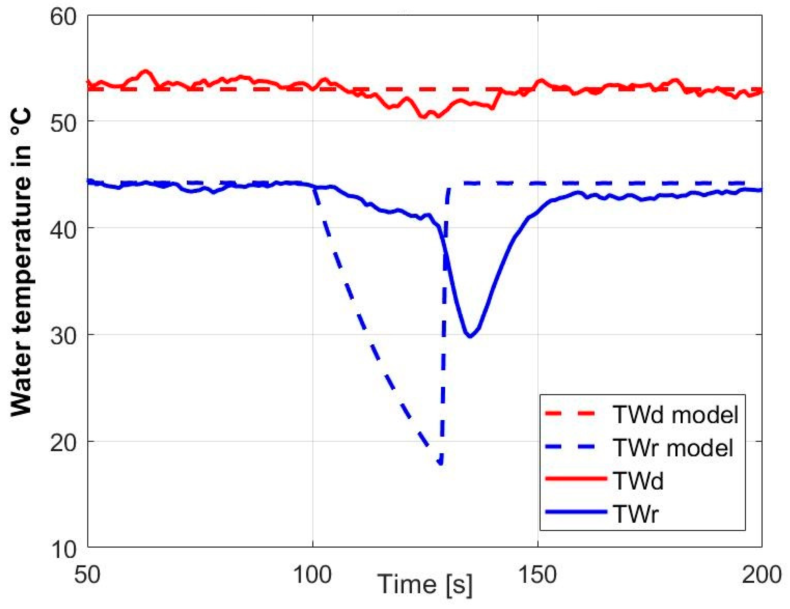
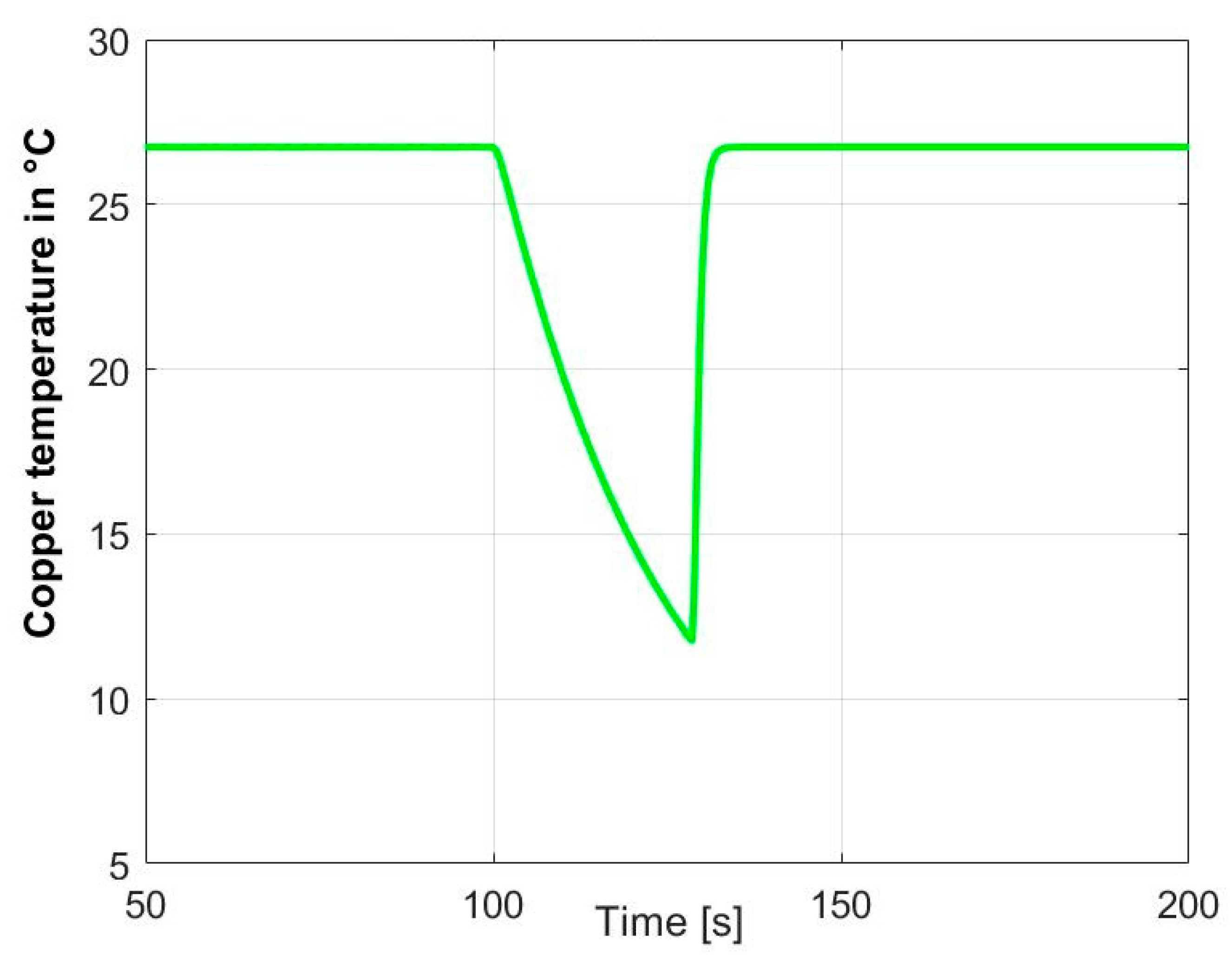
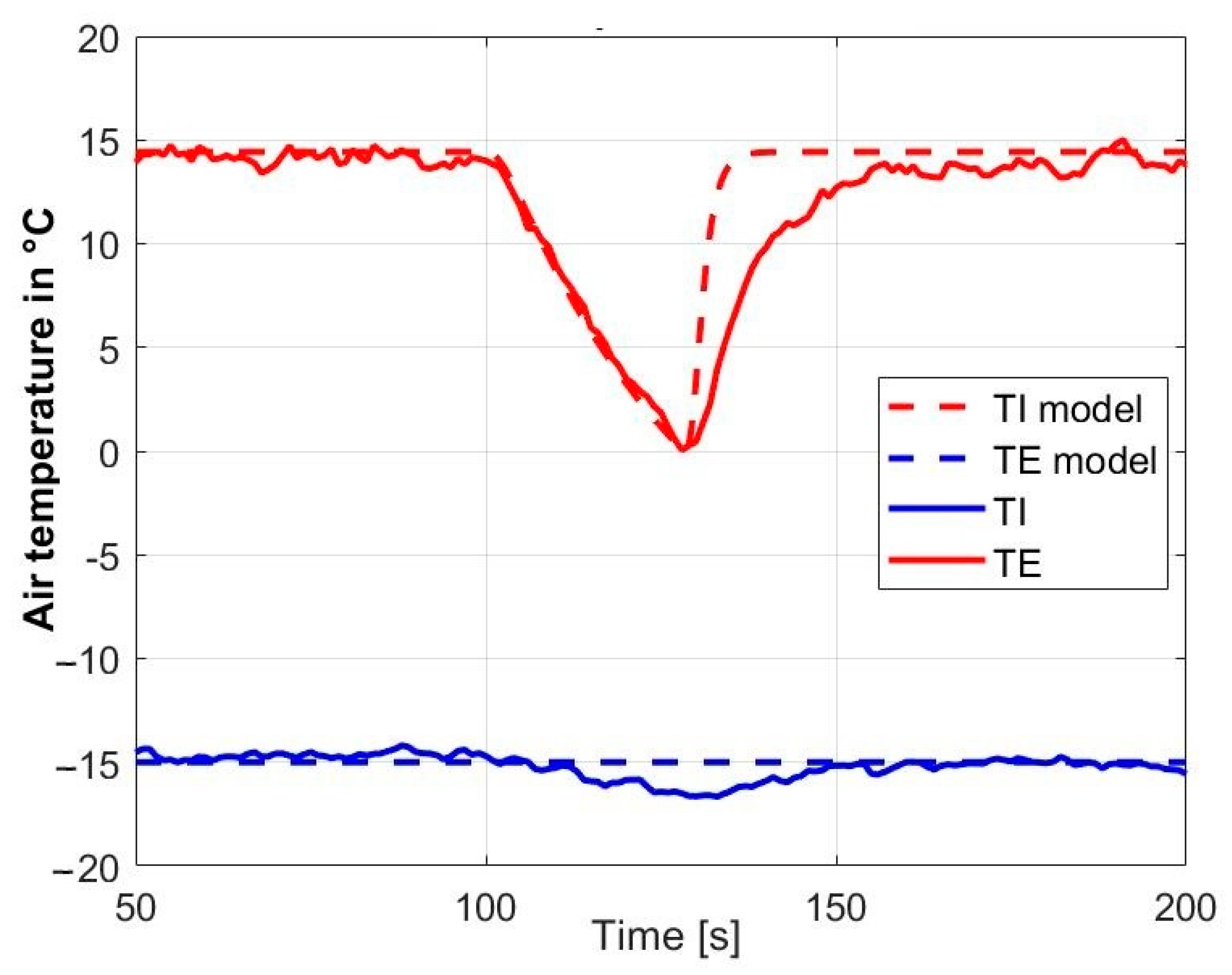
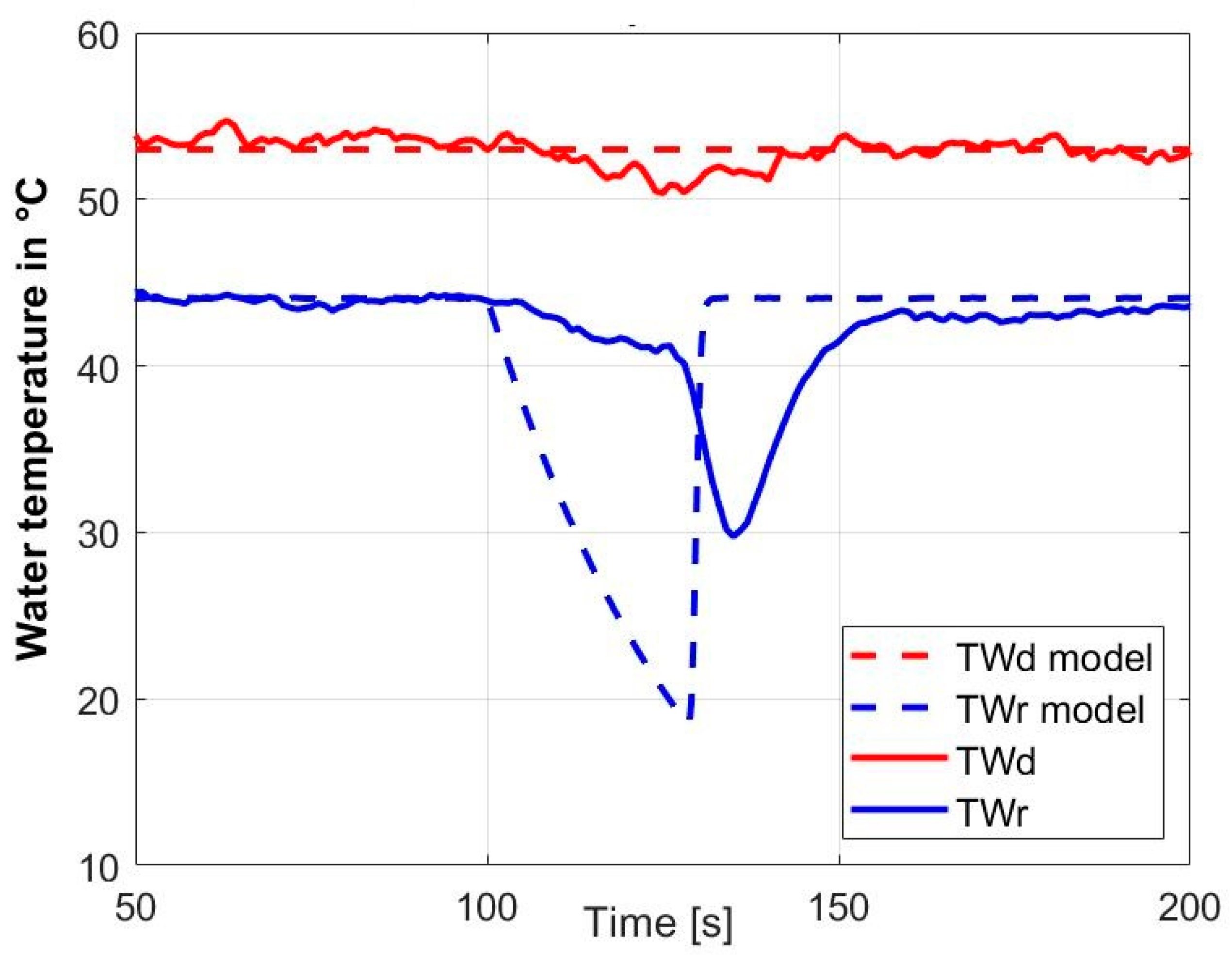
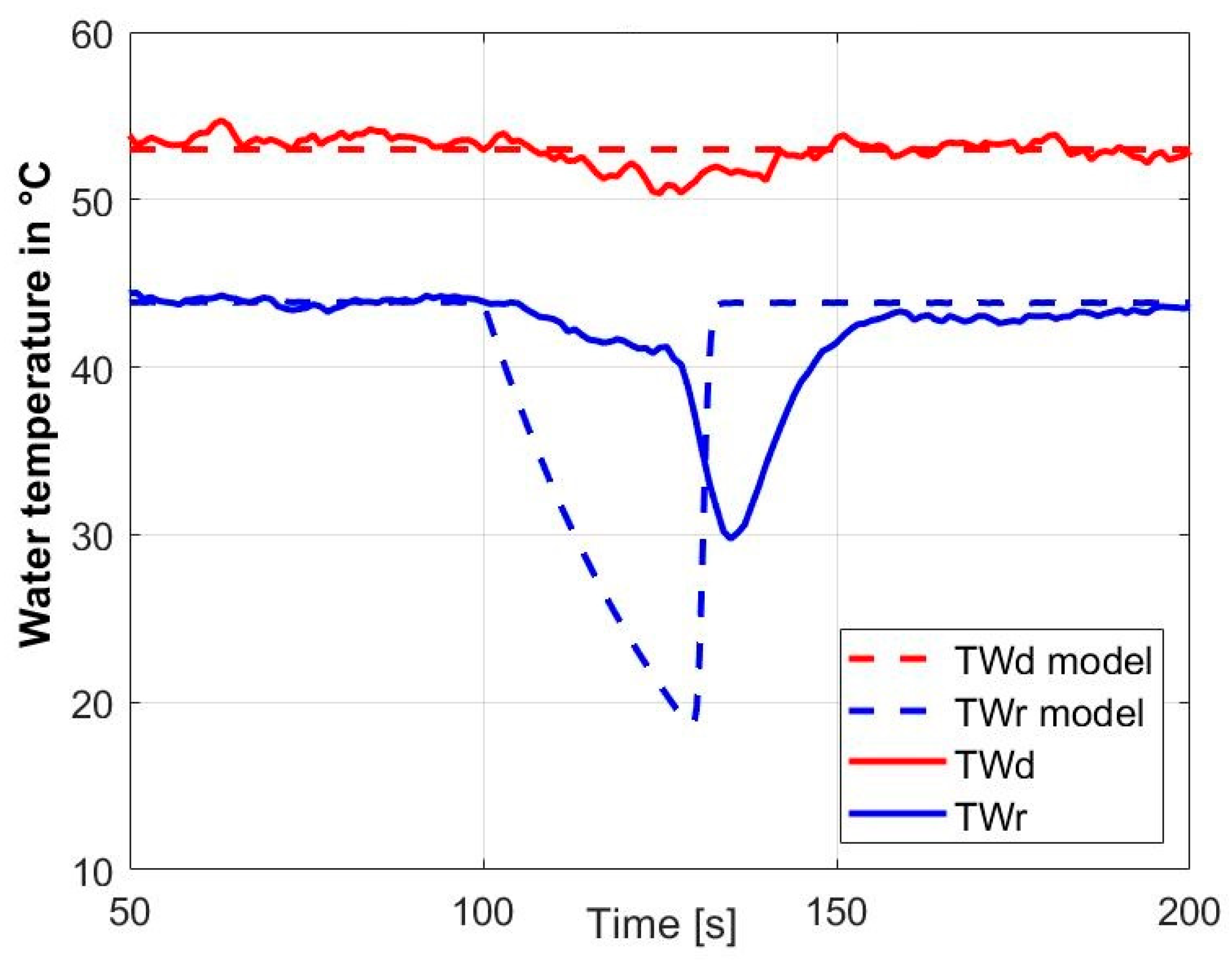
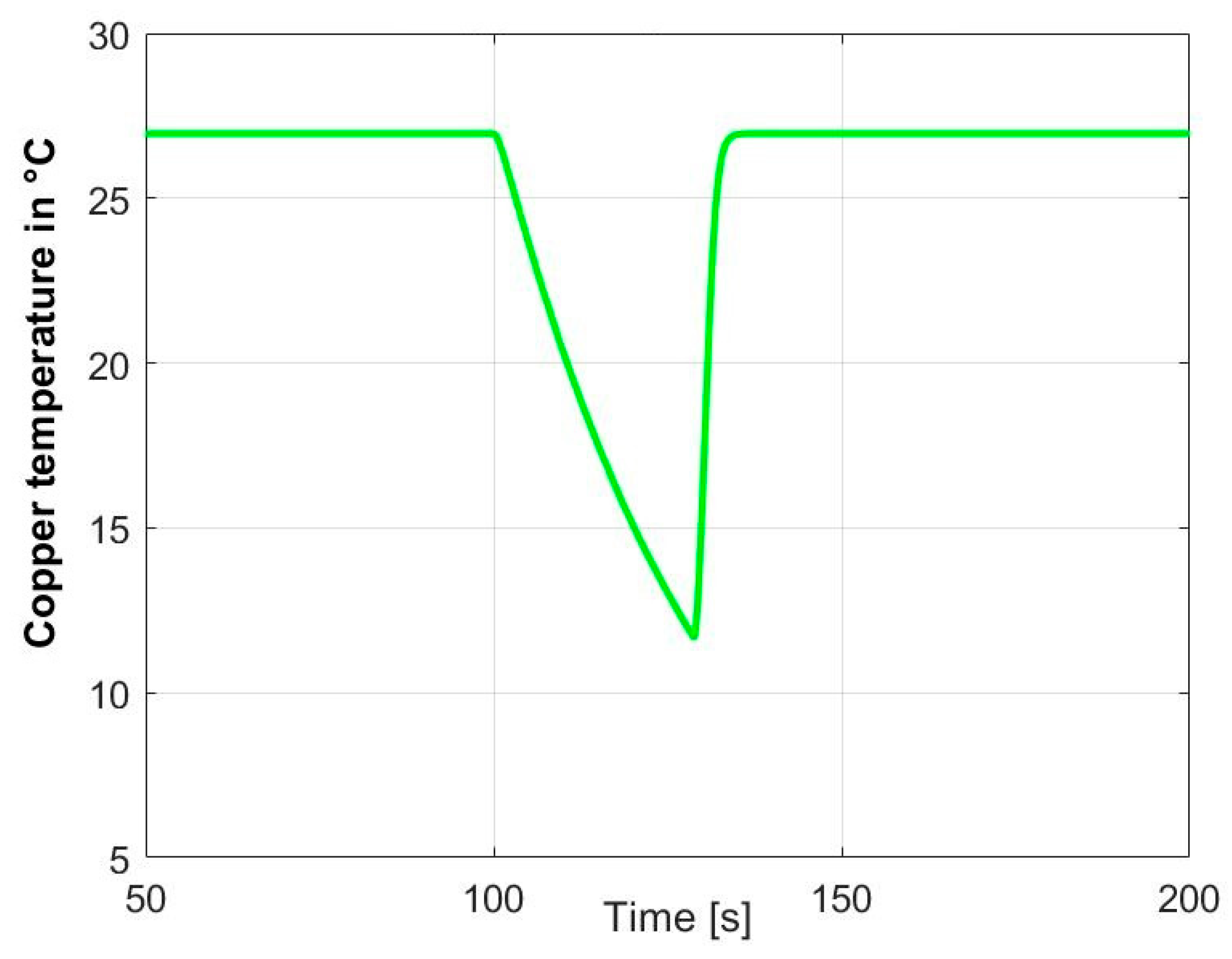
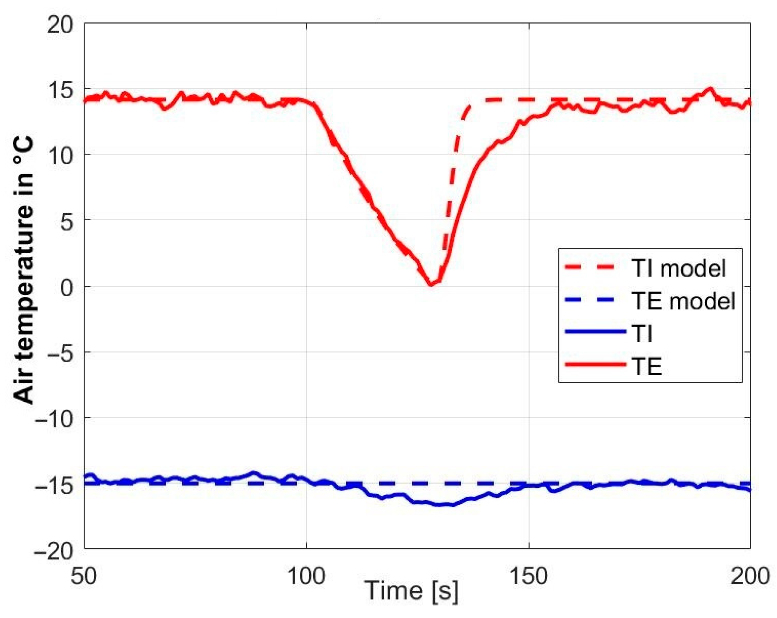
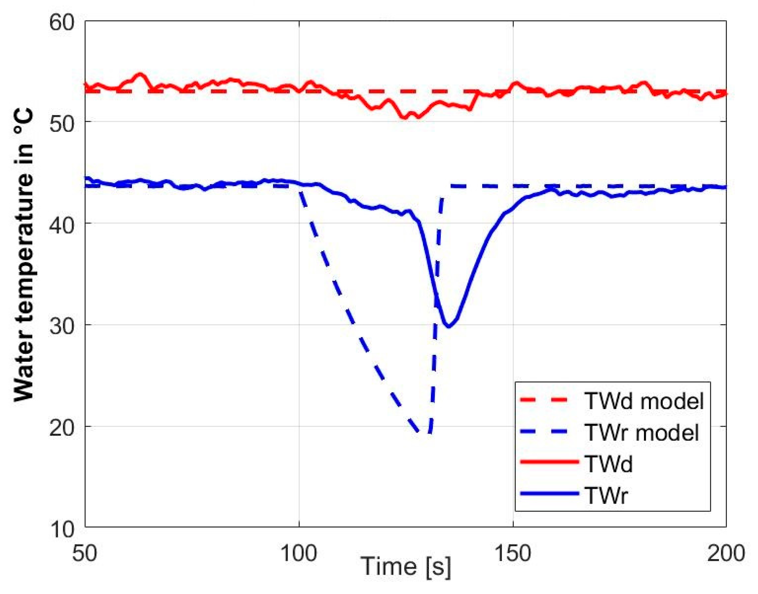
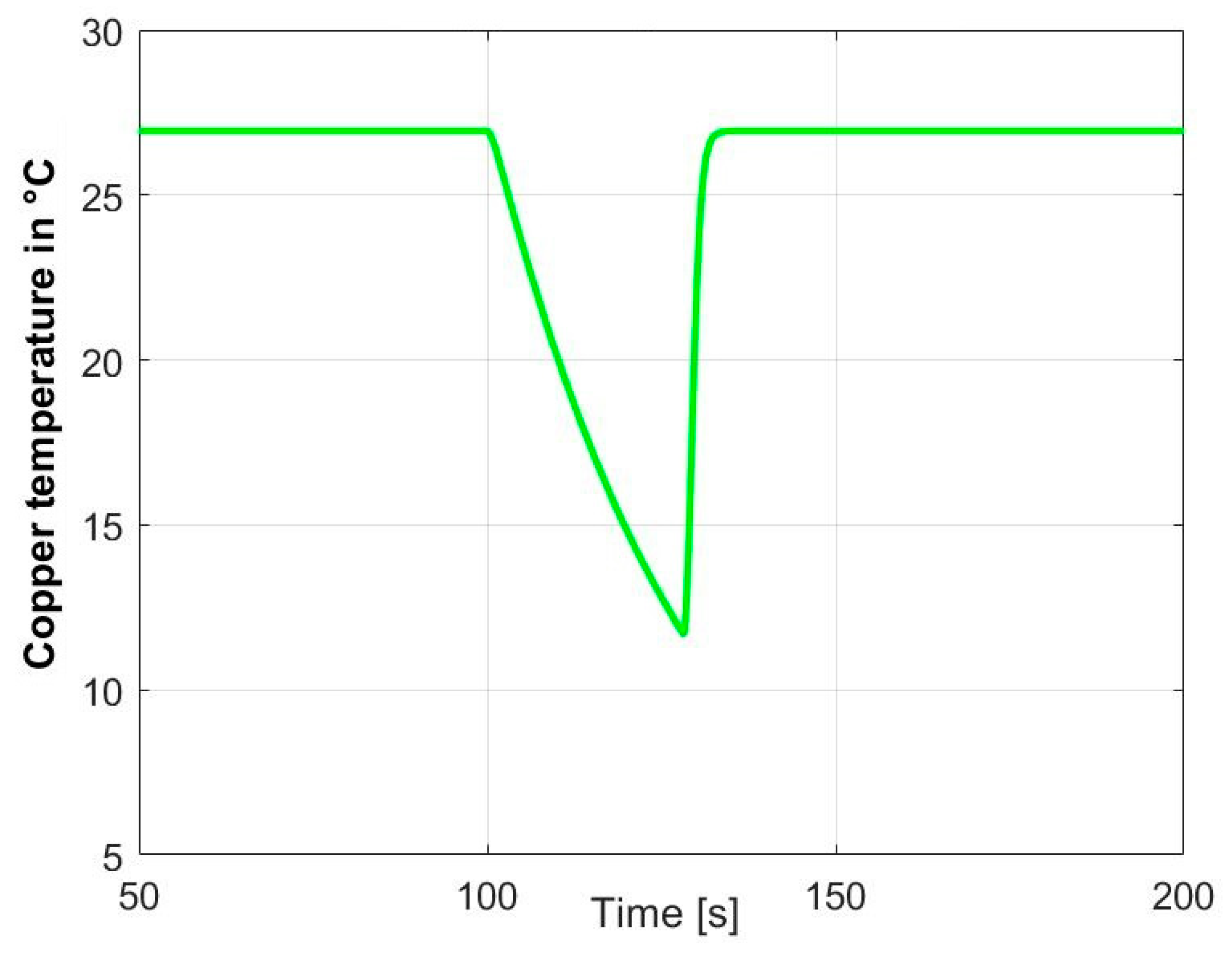
Figure 8, Figure 9, Figure 10, Figure 11, Figure 12, Figure 13, Figure 14, Figure 15, Figure 16, Figure 17, Figure 18 and Figure 19 show the results by using n = 5, 10, 15, 20 with the time of flow rate switch-off at t = 100 s, where n is the number of sections in which the water pipe of the heat exchanger was subdivided. In the diagrams, TWd is water inlet temperature, TWr is the heat exchanger outlet water temperature, TI is air inlet temperature, and TE is air outlet temperature. In addition, copper temperature diagrams have been shown.

From the results, it is possible to notice that the number of sections n does not influence much the results of the simulation, probably because this parameter has been kept low (the maximum number of sections has been chosen as 20).

However, it is worth noting that, even with a reduced number of sections, the calibrated model is able to predict the trigger of a low temperature (TL) sensor when the temperature TE gets to 0 °C after the valve shut-off. Air temperature predicted accurate curve results, showing good dynamic performance of the model. This provides an interesting application for the model, which can be employed for failure prediction in air–water heat exchangers. The modelling framework developed in this work can be helpful in designing a fault detection system.

Concerning the temperature of the water, the model predicts a higher temperature of the outflow water. This may be ascribed to the fact that typically nonlinear effects are neglected, such as those due to the fluid inertia.

The valve closure does not provide an instantaneous drop in water temperature, which partially continues to flow in a small but non-null time, as differently accounted in the model. This may be ascribed to the fact that parameters as fluid inertia and valve closure time are neglected. The behavior over time of the outflow water temperature TWr can be obtained by the same linear model using a nonzero flow.

Based on the aforesaid, a TL sensor in the air flow with triggering at 0 °C, including an adequate margin to account for sensor standard imprecision, is well-suited to ensure safe use of the coil system because of the worst-case pessimistic conditions adopted in developing and tuning the model.

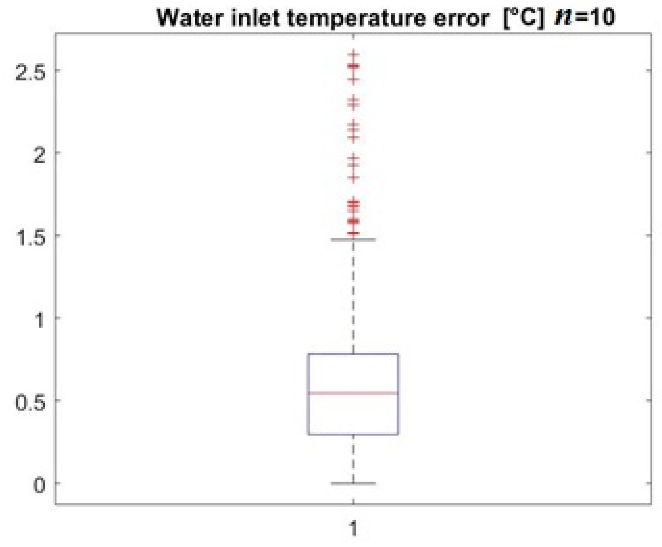
Error analysis was performed for an intermediate case, namely the n = 10 case; the data analyzed was water temperature, representing the variable which presents the most accentuated errors between the measured and the simulated data.

Error analysis was done by using the “boxplot” command in Matlab, which presents the median, the 25th percentile, the 75th percentile, and the outlier data in the same picture. Figure 20 shows the error analysis for the water inlet temperature as a comparative case.

As visible, in the case of the water inlet temperature, the errors between the model outputs and the real data are limited within the range of +2.5 °C, with an error median of 0.54 °C and mean equal to 0.63 °C.

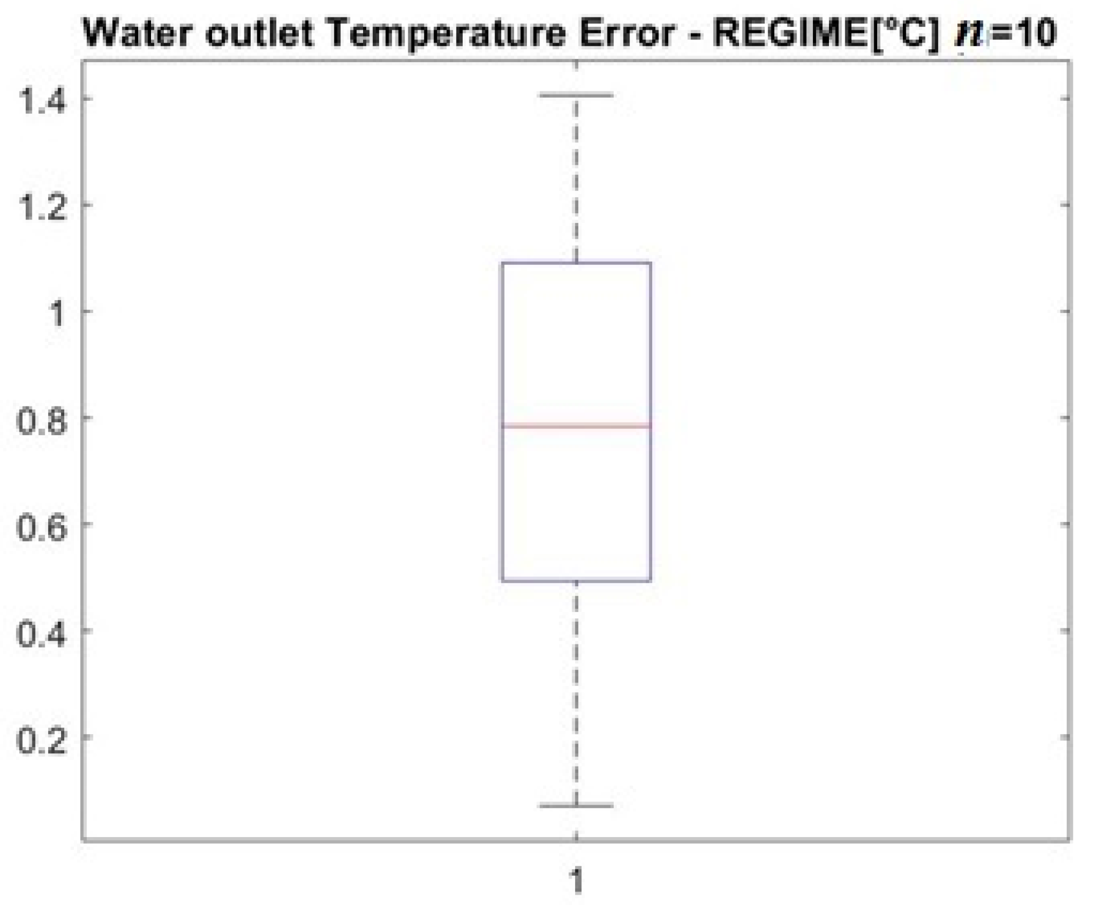
Then, the analysis was performed for the water outlet temperature, the behavior of which can be divided into three main intervals: first, temperature remains constant; then, between 100 and 130 s, there is a second interval with a temperature drop owing to the valve closure; finally, a third interval occurs, where temperature is about constant.

The analysis was made separately for the central interval in which the transient occurs (called “transient” in the images) and for the two time intervals where temperature is constant (called “regime”).

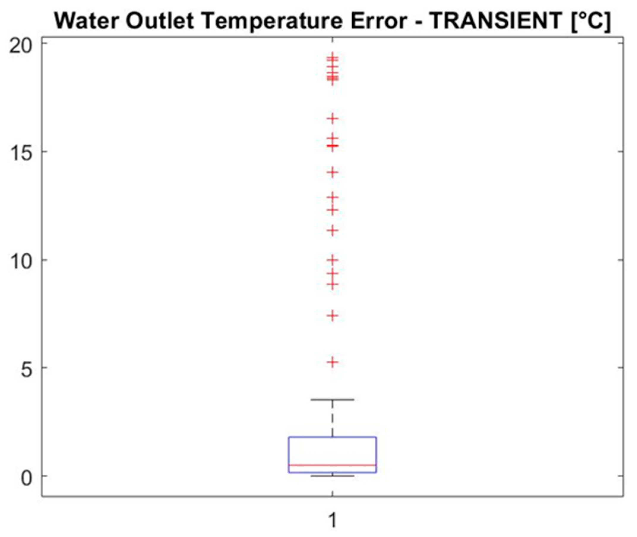
As visible in Figure 21, the median in the regime zone is 0.8 °C, with a mean error of 0.78 °C and peaks of about 1.4 °C. Figure 22 highlights how in transient condition, the median stands in about 1 °C; the mean is 3.19 °C, but the peak error values reach about 20 °C. This highlights that the model is accurate in predicting the water temperature values at regime conditions, but presents significant errors in the transient conditions. Thus, future work will be devoted to improving precision in modelling the transient behavior, which can be made by more careful identification.

4. Conclusions

This paper presents a model based on Laplacian transform discretization of the balance equations to simulate the behavior of the main variables of a cross-flow heat exchanger finalized to heat the air flow feeding an air conditioning system operating in low temperature environments.

After a literature review, the paper describes the model and its fundamental parameters, other than the methodology employed for modelling, including the discretization of the balance equations with Laplace transform. Laplace transform is useful because the discretization of the governing equations by this method permits to treat different configurations of the heat exchanger, sub-dividing it into ranks and reproducing the bi-dimensional extension of a cross-flow heat exchanger. Then, the description continues with the calibration of the model control parameters based on real data coming from the sensors installed in the system. Finally, the model functionality is tested, comparing the model output signals with on-field experimental data, for different numbers of elements in which the modeled pipe has been subdivided.

The results provided by the model show that the aim of the article, which was to implement a model able to simulate the dynamic behavior of the temperatures to changing external conditions, is accomplished, as the change in air temperature to water flow rate variation was accurate with respect to the experimental data, correctly predicting the negative peak of air temperature to the shut-off of the hot water. This accomplishes the initial purpose—to provide an accurate parameter to be exploited in avoiding damages to the system; for example, feed-water freezing.

The strengths of this model are its simplicity in implementation, rapid computing, and flexibility in representing different geometrical configurations of heat exchangers.

Future work will provide model modifications for better prediction during transients. The precision in transient reproduction can be improved by more careful identification. Based on the preliminary results obtained by the model described in this article, another improvement may be the development of a concentrated parameter model based on partial differential equations.