
A Case Study of Open- and Closed-Loop Control of Hydrostatic Transmission with Proportional Valve Start-Up Process

 ,
,  ,
,  ,
,  and
and
Abstract
1. Introduction
Hydrostatic Transmission Control Methods
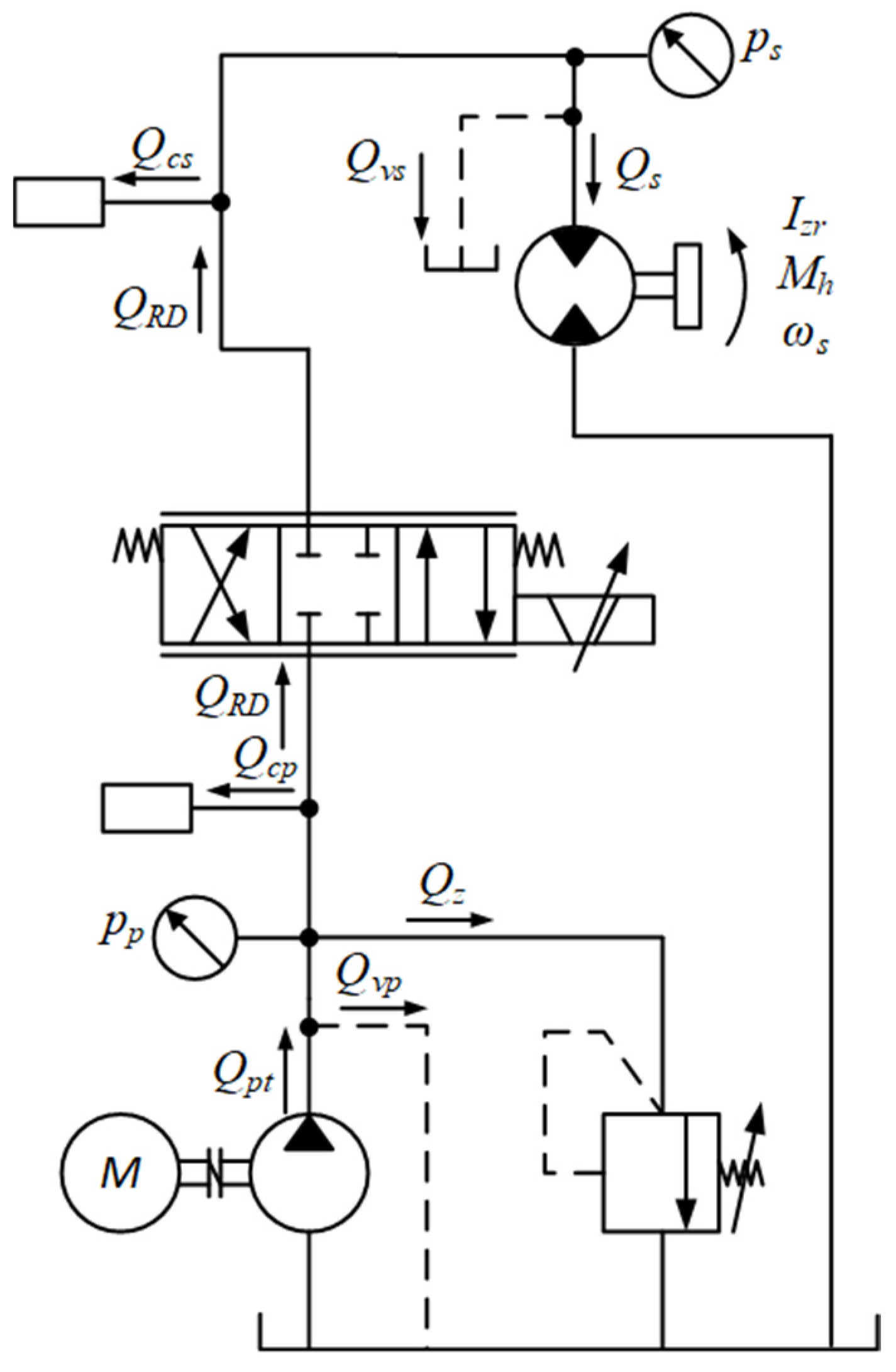
2. Mathematical Model for the Serial Throttle Control Method
- The temperature of the medium, and consequently its viscosity, remains constant throughout the simulation;
- The pressure has no effect on the viscosity of the medium;
- The compressibility of the medium and the deformability of the hydraulic elements was reduced to the concentrated capacitance at particular points of the system;
- There is no air in the system;
- There is no backlash in the mechanical system;
- The load of the motor is focused on its shaft (inertia);
- There are no wave phenomena;
- There are no external leaks in the system;
- The speed of the electric motor driving the pump is constant and is independent of the pump load;
- On the section from the pump to the proportional spool valve:
- On the section from the proportional spool valve to the motor:
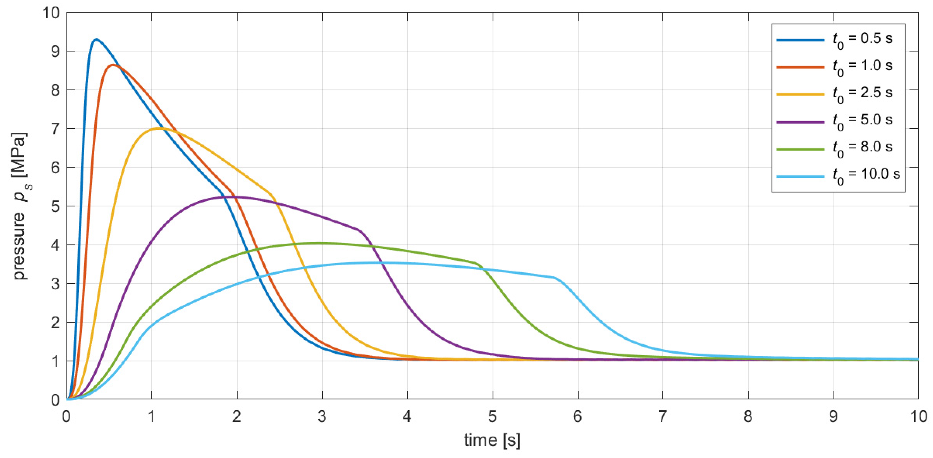
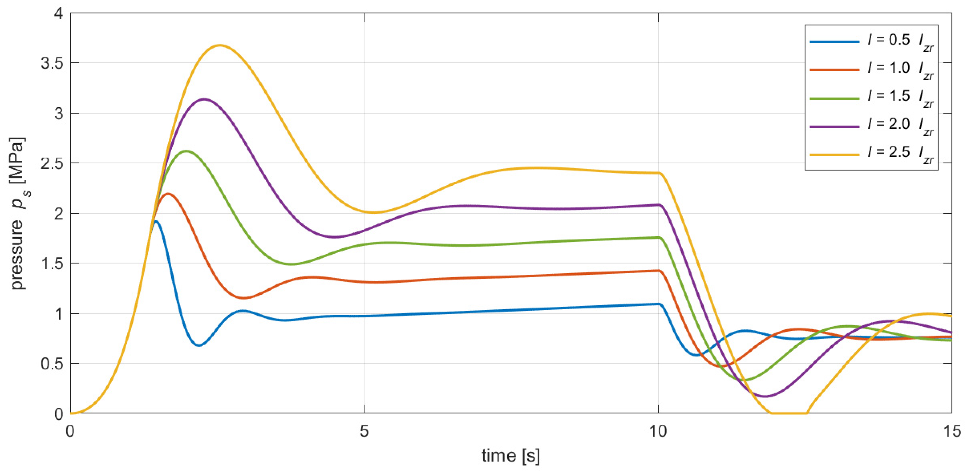
- Dynamic surplus pressure as the maximum pressure recorded during the start-up phase;
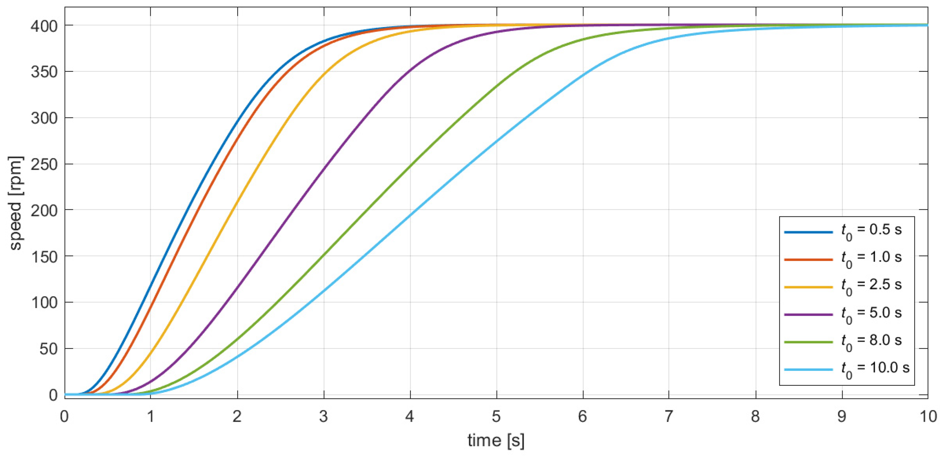
- Start-up time as the time after which the rotational speed reaches 95% of the set value from the moment of supplying the control signal;
- Reaction time as the time after which the speed of the motor reaches 5% of the set value;
- Energy generated by the pump during the start-up process (first 10 s).
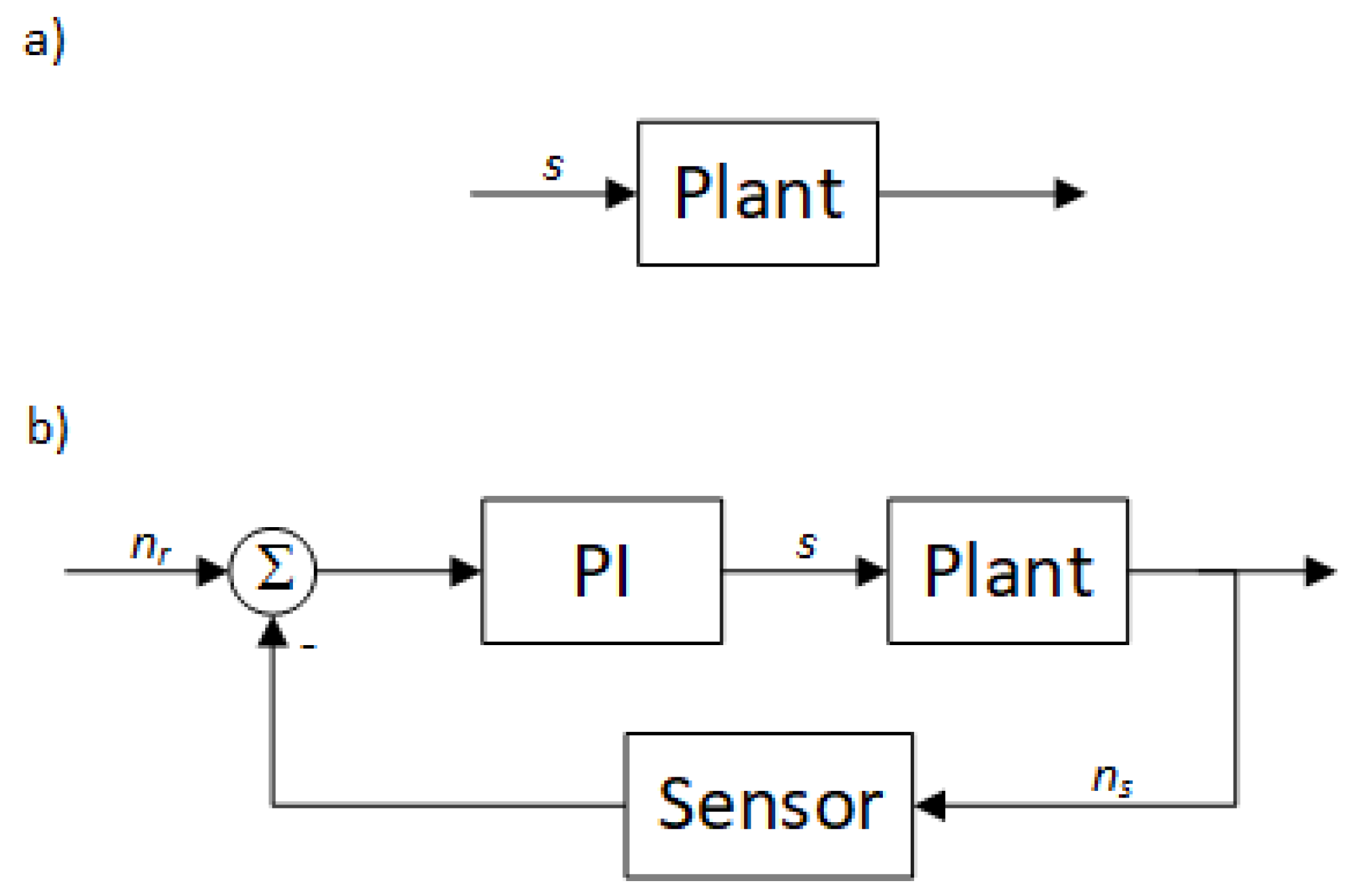
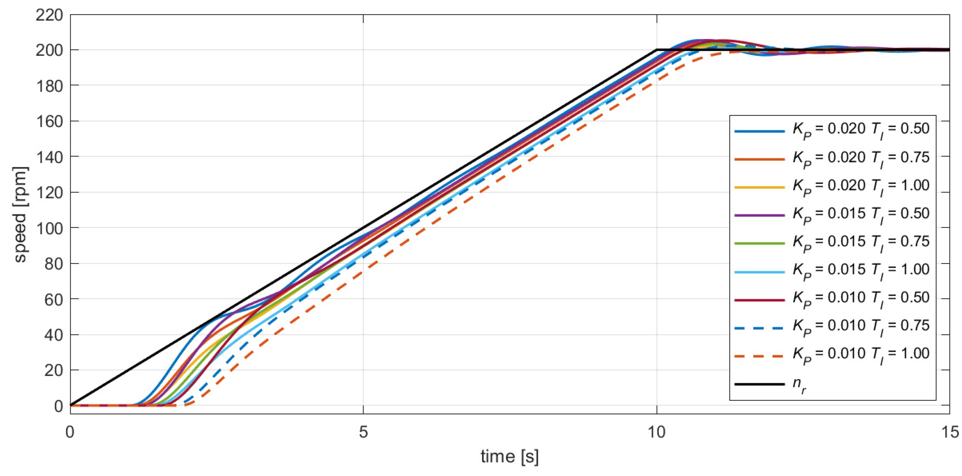
- Overshoot parameter described by the following relation:
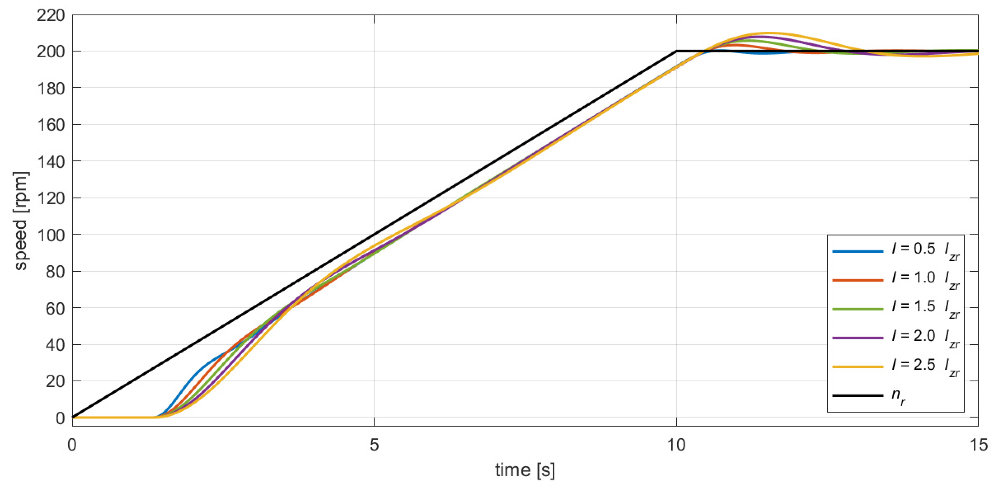
- Steady-state error for the ramp input measured at the end of the ramp signal:
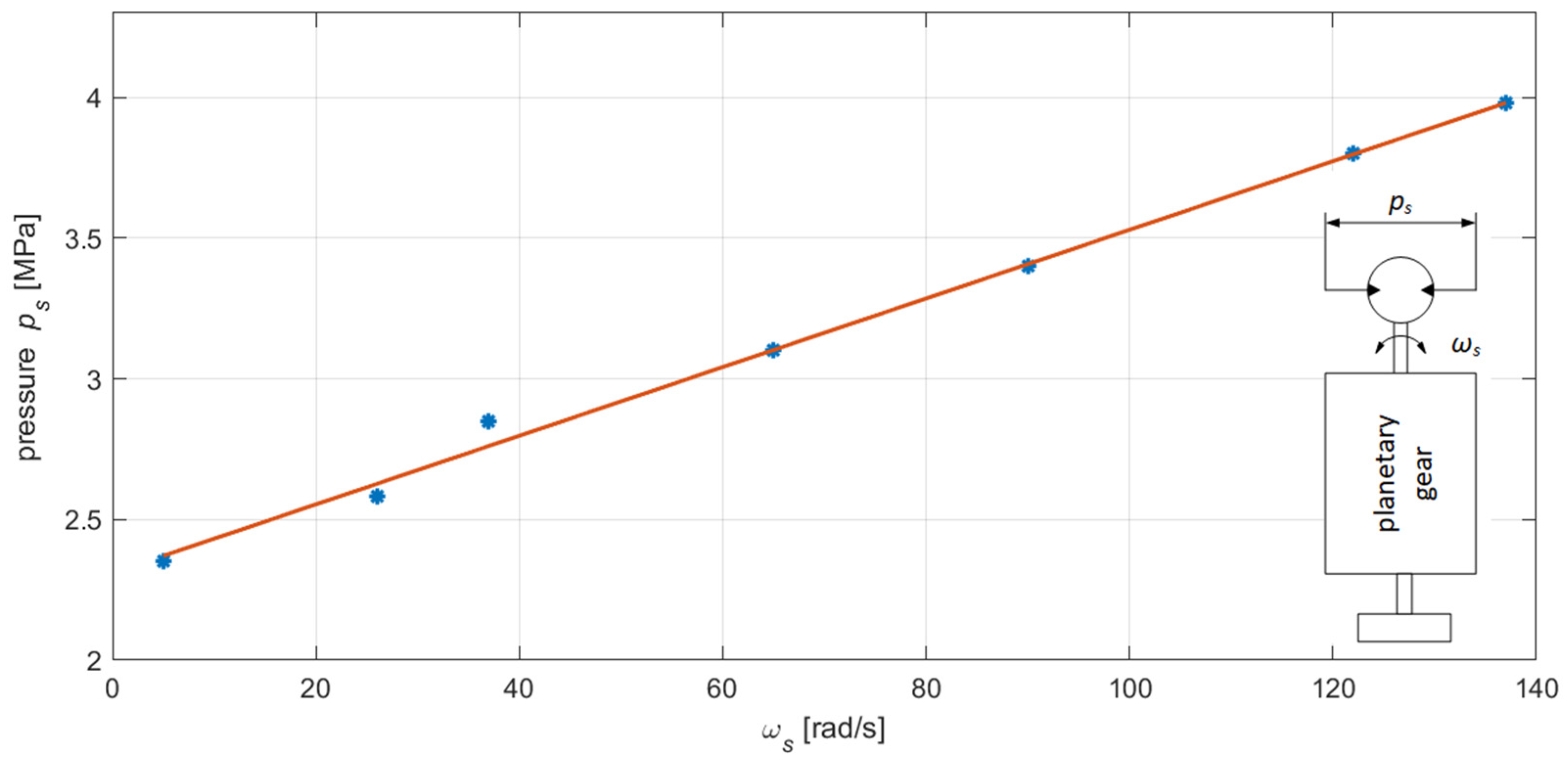
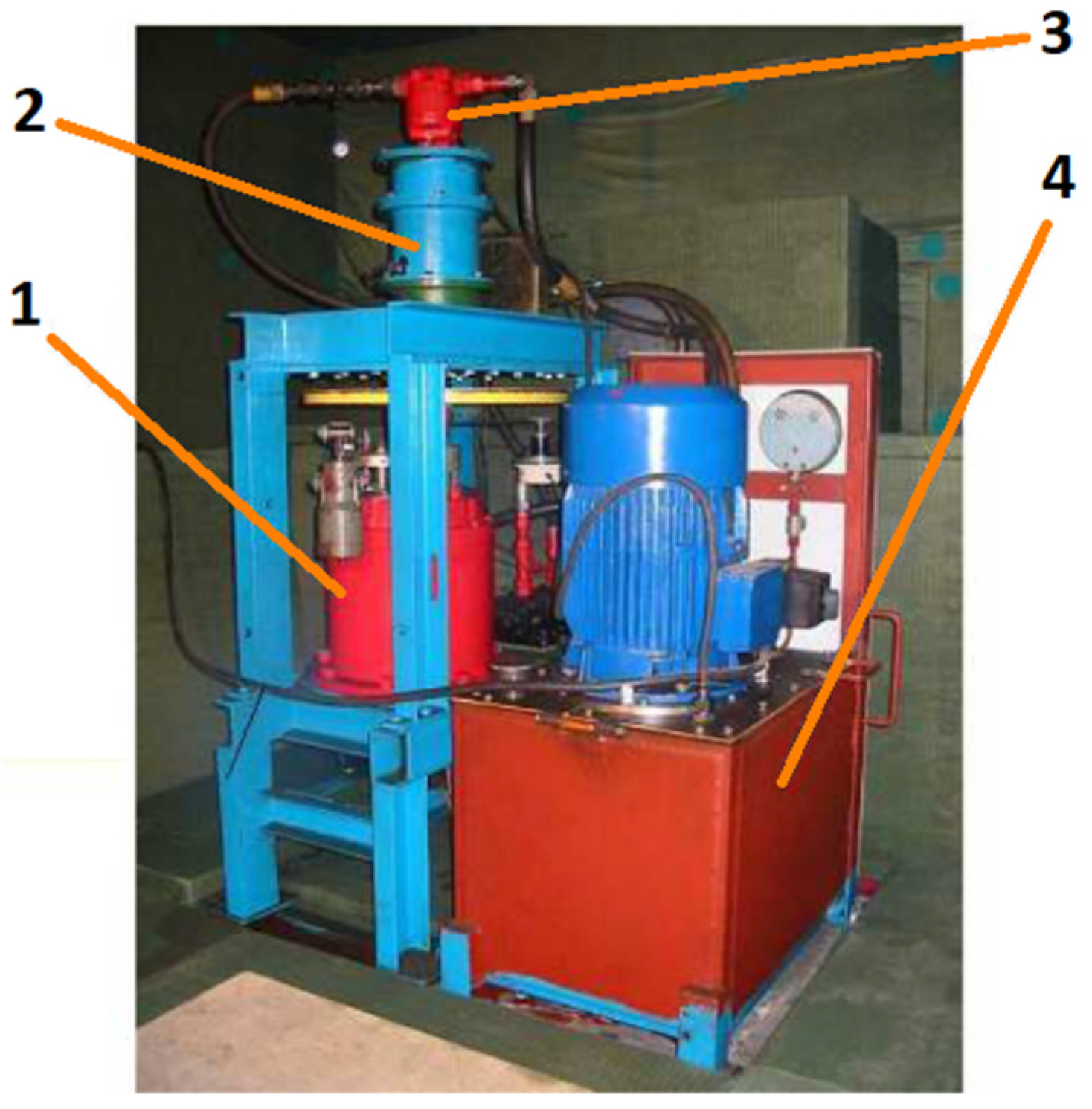
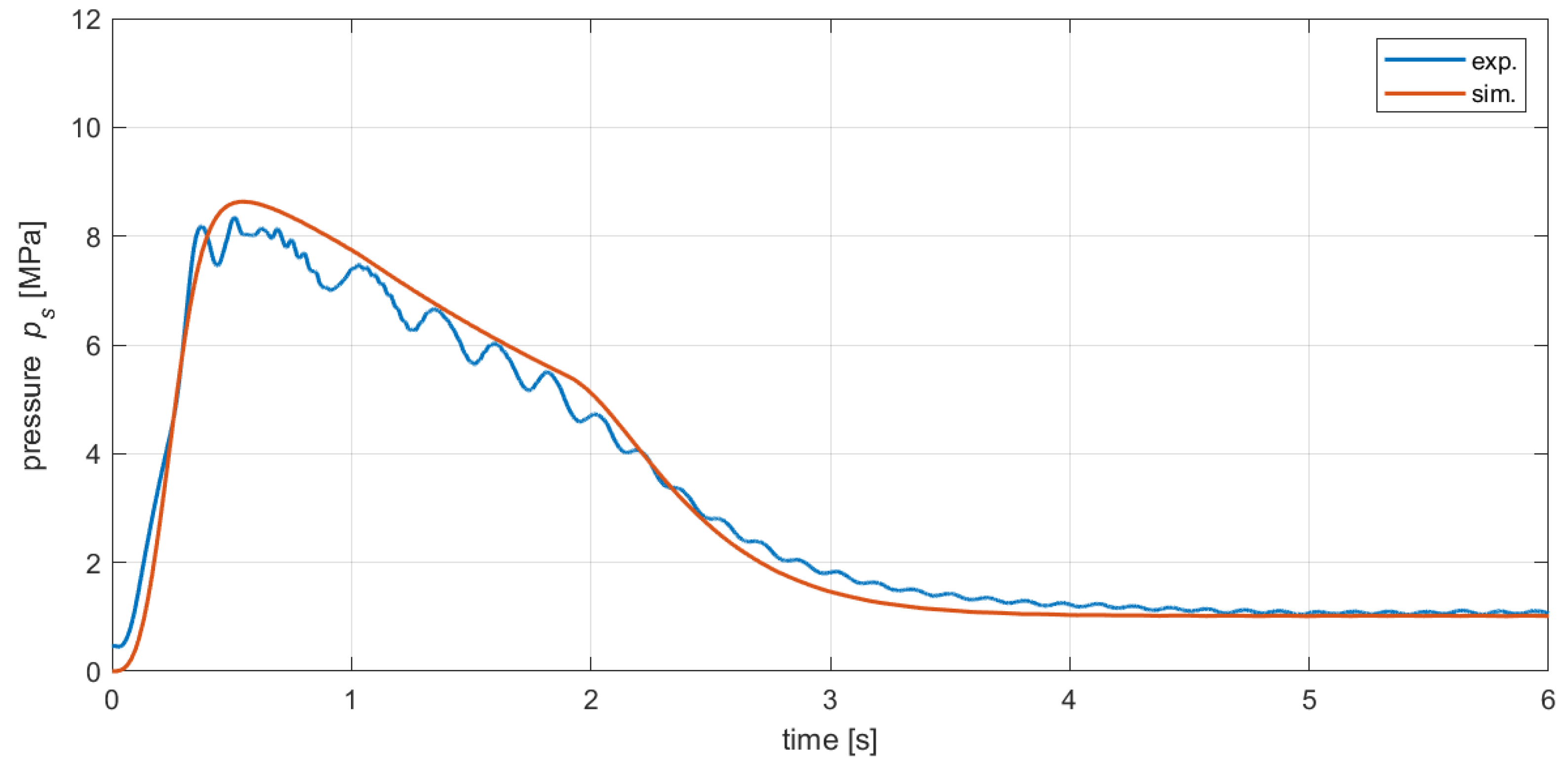
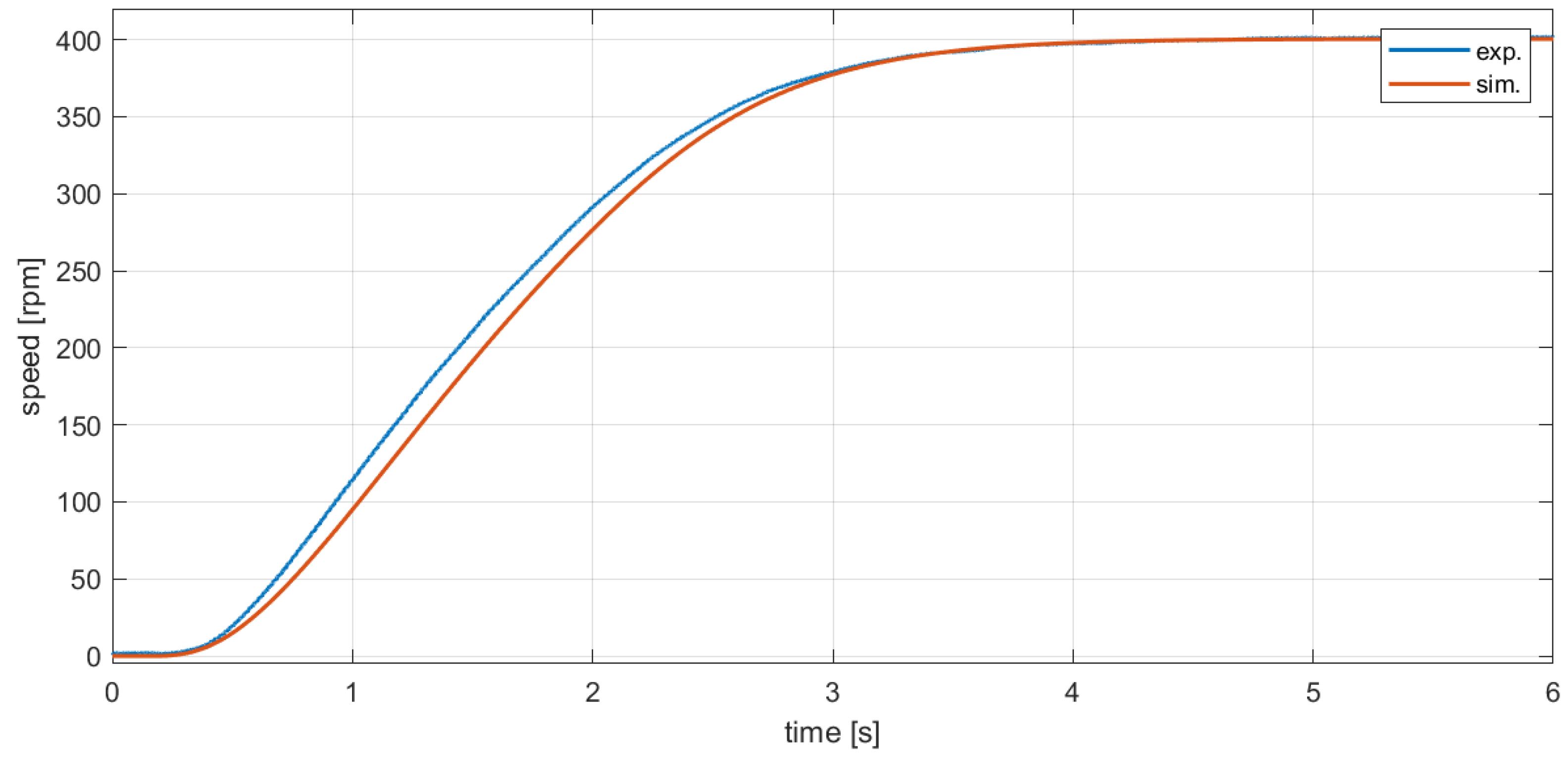
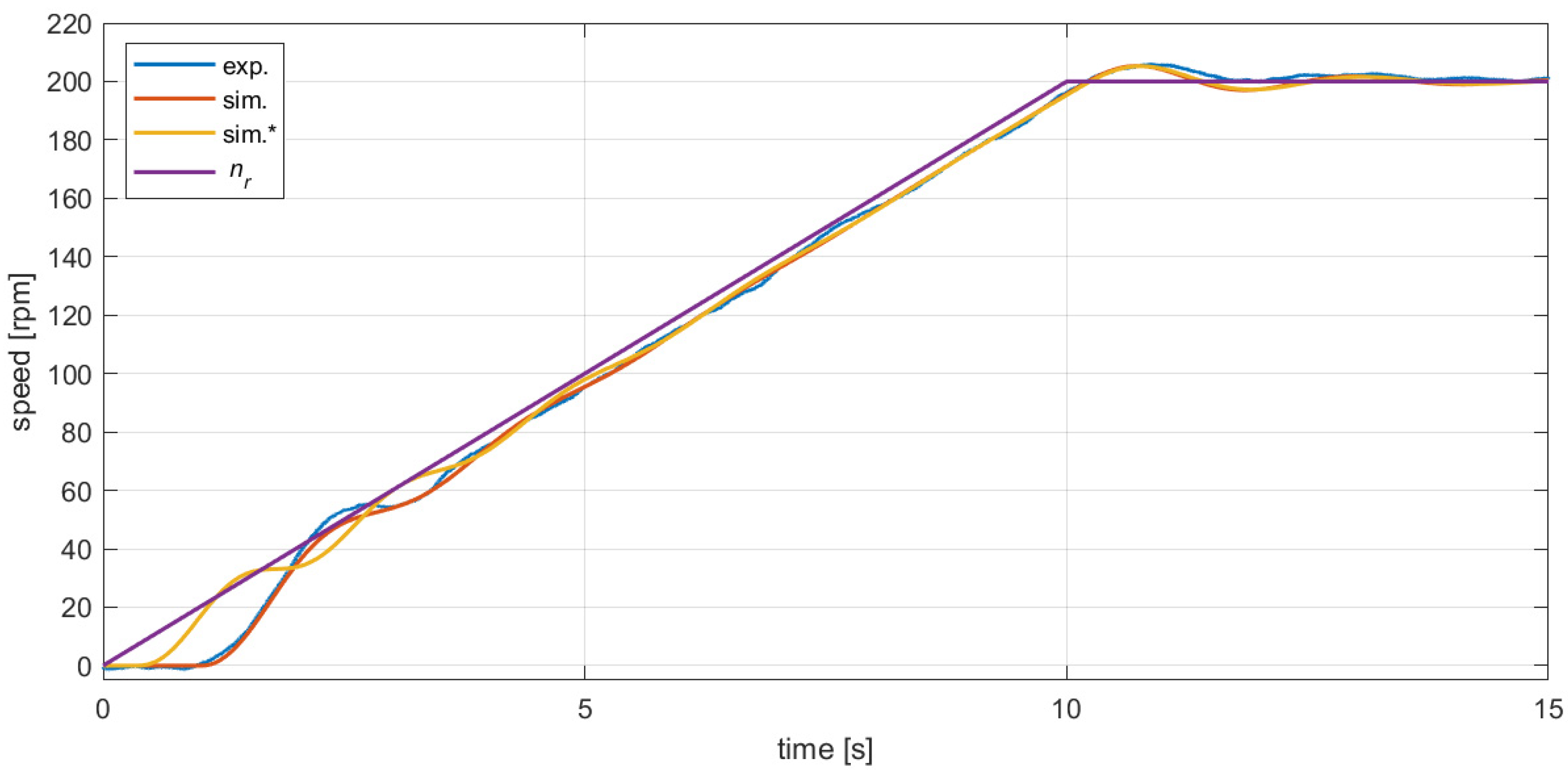
3. Experimental Verification of the Mathematical Model
4. Conclusions
Author Contributions
Funding
Institutional Review Board Statement
Informed Consent Statement
Data Availability Statement
Conflicts of Interest
Nomenclature
| pump leakage coefficient | |
| motor leakage coefficient | |
| coefficients of the polynomial function describing the opening of the spool valve | |
| capacitance of the liquid and of the pipes on the section from the pump to the proportional spool valve | |
| capacitance of the liquid and of the pipes on the section from the proportional spool valve to the motor | |
| steady-state error to ramp input | |
| energy generated by the pump during the first 10 s | |
| viscous friction coefficient | |
| transmittance of the rotational speed measuring system | |
| PI controller transmittance | |
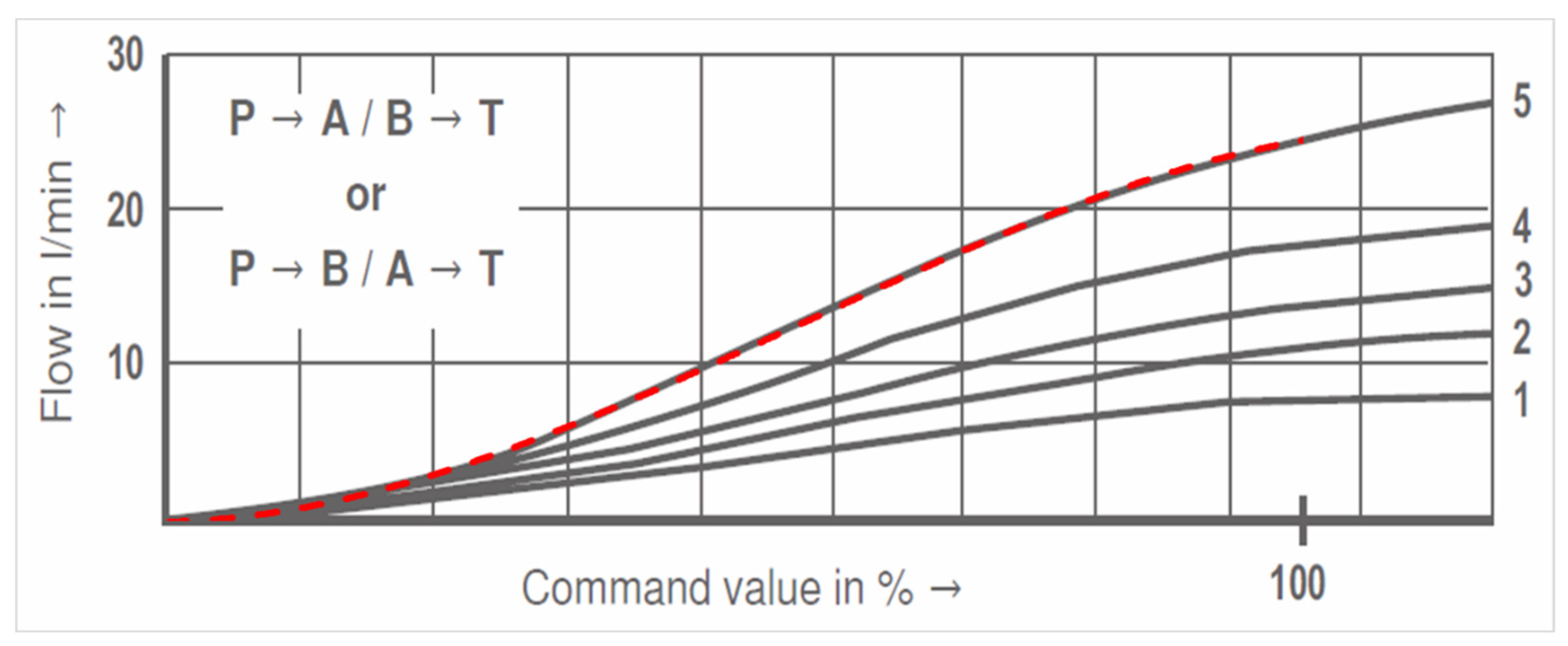
| conductivity of the spool valve | |
| maximum conductivity of the spool valve | |
| amplification factor of the relief valve | |
| gear ratio of the planetary gear | |
| j | summation index |
| minimum value of the control signal | |
| maximum value of the control signal | |
| reduced mass moment of inertia of rotational masses | |
| proportional gain of the PI controller | |
| braking torque on the shaft of the hydrostatic motor | |
| total length of the pipes between the pump and the motor | |
| rotational speed of the hydrostatic motor | |
| initial rotational speed in the controlled system | |
| target rotational speed in the controlled system | |
| current rotational speed set point in the controlled system | |
| rotational speed on the shaft of the hydrostatic motor | |
| opening pressure of the relief valve | |
| total pressure drop resulting from flow rate losses | |
| pressure on the pump | |
| pressure on the hydraulic motor | |
| dynamic surplus pressure on the motor | |
| pressure at the hydraulic motor corresponding to static resistance values (for ) | |
| inner radius of the hydraulic pipes | |
| control signal | |
| modified control signal | |
| simulation time (step) | |
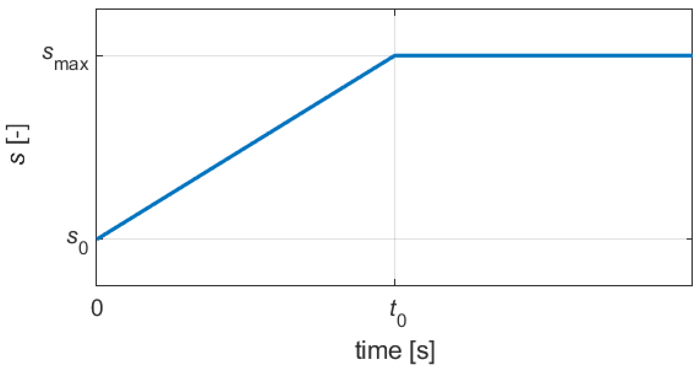
| control signal edge rise time | |
| oil temperature in the planetary gear | |
| oil temperature in the hydraulic system | |
| transmission reaction time | |
| transmission start-up time | |
| time constant of the integrating element of the PI controller | |
| time constant of the system for measuring the rotational speed | |
| time constant of the spool valve | |
| time constant of the relief valve | |
| displacement of the hydraulic motor | |
| theoretical pump output flow | |
| flow value resulting from losses in the pump | |
| flow through the relief valve | |
| flow through the proportional valve | |
| flow caused by compressibility in volume between the pump and the spool valve | |
| flow caused by the compressibility in volume between the proportional spool valve and the hydraulic motor | |
| flow towards the hydraulic motor | |
| flow value resulting from losses in the hydraulic motor | |
| coefficient of pressure losses caused by turbulent flow | |
| speed overshoot in a PI controlled system | |
| dynamic viscosity of the working medium | |
| density of the working medium | |
| angular velocity of the hydrostatic motor |
References
- Pullen, K.R.; Dhand, A. Mechanical and Electrical Flywheel Hybrid Technology to Store Energy in Vehicles. In Alternative Fuels and Advanced Vehicle Technologies for Improved Environmental Performance; Elsevier: Amsterdam, The Netherlands, 2014; pp. 476–504. ISBN 978-0-85709-522-0. [Google Scholar]
- Comellas, M.; Pijuan, J.; Potau, X.; Noguès, M.; Roca, J. Efficiency sensitivity analysis of a hydrostatic transmission for an off-road multiple axle vehicle. Int. J. Automot. Technol. 2013, 14, 151–161. [Google Scholar] [CrossRef]
- Xiong, S.; Wilfong, G.; Lumkes, J.J. Components Sizing and Performance Analysis of Hydro-Mechanical Power Split Transmission Applied to a Wheel Loader. Energies 2019, 12, 1613. [Google Scholar] [CrossRef]
- Hubballi, B.; Sondur, V. Noise Control in Oil Hydraulic System. In Proceedings of the 2017 International Conference on Hydraulics and Pneumatics-HERVEX, Băile Govora, Romania, 8–10 November 2017, ISSN 1454-8003. [Google Scholar]
- Liu, J.; Yang, Y.; Suh, S. Hydraulic Fluid-Borne Noise Measurement and Simulation for Off-Highway Equipment. In Proceedings of the 2017 SAE/NOISE-CON Joint Conference (NoiseCon 2017), Grand Rapids, MI, USA, 11 June 2017. [Google Scholar]
- Fiebig, W.; Wrobel, J. System Approach in Noise Reduction in Fluid Power Units. In Proceedings of the BATH/ASME 2018 Symposium on Fluid Power and Motion Control, Bath, UK, 12–14 September 2018; American Society of Mechanical Engineers: Bath, UK, 12 September 2018; p. V001T01A025. [Google Scholar]
- Wróbel, J.; Blaut, J. Influence of Pressure Inside a Hydraulic Line on Its Natural Frequencies and Mode Shapes. In Advances in Hydraulic and Pneumatic Drives and Control 2020; Stryczek, J., Warzyńska, U., Eds.; Lecture Notes in Mechanical Engineering; Springer International Publishing: Cham, Switzerland, 2021; pp. 333–343. ISBN 978-3-030-59508-1. [Google Scholar]
- Fiebig, W.; Wrobel, J.; Cependa, P. Transmission of Fluid Borne Noise in the Reservoir. In Proceedings of the BATH/ASME 2018 Symposium on Fluid Power and Motion Control, Bath, UK, 12–14 September 2018; American Society of Mechanical Engineers: Bath, UK, 12 September 2018; p. V001T01A026. [Google Scholar]
- Zarzycki, Z.; Urbanowicz, K. Modelling of transient flow during water hammer considering cavitation in pressure pipes. Inżynieria Chem. I Proces. 2006, 27, 915–933. [Google Scholar]
- Makaryants, G.M.; Prokofiev, A.B.; Shakhmatov, E. Vibroacoustics Analysis of Punching Machine Hydraulic Piping. Procedia Eng. 2015, 106, 17–26. [Google Scholar] [CrossRef][Green Version]
- Skorek, G. Study of Losses and Energy Efficiency of Hydrostatic Drives with Hydraulic Cylinder. Pol. Marit. Res. 2018, 25, 114–128. [Google Scholar] [CrossRef]
- Karpenko, M.; Bogdevičius, M. Review of Energy-saving Technologies in Modern Hydraulic Drives. Moksl.-Liet. Ateitis 2017, 9, 553–558. [Google Scholar] [CrossRef]
- Karpenko, M.; Bogdevičius, M. The Hydraulic Energy-Saving System Based on the Hydraulic Impact Effect. In Proceedings of the 10th National Conferences “Jūros ir krantų Tyrimai”, Palanga, Lithuanian, 26–28 April 2017. [Google Scholar]
- Lin, T.; Chen, Q.; Ren, H.; Miao, C.; Chen, Q.; Fu, S. Influence of the energy regeneration unit on pressure characteristics for a proportional relief valve. Proc. Inst. Mech. Eng. Part I J. Syst. Control. Eng. 2017, 231, 189–198. [Google Scholar] [CrossRef]
- Domagała, Z.; Kędzia, K.; Stosiak, M. The use of innovative solutions improving selected energy or environmental indices of hydrostatic drives. IOP Conf. Ser. Mater. Sci. Eng. 2019, 679, 012016. [Google Scholar] [CrossRef]
- Sobczyk, A.; Pobędza, J. Hydraulic Systems Safety by Reducing Operation and Maintenance Mistakes. Syst. Saf. Hum.-Tech. Facil.-Environ. 2019, 1, 700–707. [Google Scholar] [CrossRef]
- Larsson, L.V. Control of Hybrid Hydromechanical Transmissions; Linköping Studies in Science and Technology; Division of Fluid and Mechatronic Systems, Department of Management and Engineering Linköping University: Linköping, Sweden, 2019. [Google Scholar]
- Yao, Z.; Liang, X.; Zhao, Q.; Yao, J. Adaptive Disturbance Observer-Based Control of Hydraulic Systems with Asymptotic Stability. Appl. Math. Model. 2022, 105, 226–242. [Google Scholar] [CrossRef]
- Acuna, W.; Canuto, E.; Malan, S. Embedded Model Control Applied to Mobile Hydraulic Systems. In Proceedings of the 18th Mediterranean Conference on Control and Automation, MED’10, Marrakech, Morocco, 23–25 June 2010; IEEE: Marrakech, Morocco, 2010; pp. 715–720. [Google Scholar]
- Saleem, A.M.; Alyas, B.H.; Mahmood, A.G. Mathematical Model for a Proportional Control Valve of a Hydraulic System. Int. J. Mech. Prod. Eng. Res. Dev. (IJMPERD) 2020, 10, 8433–8444. [Google Scholar]
- Tenesaca, J.; Carpio, M.; Saltarén, R.; Portilla, G. Experimental determination of the nonlinear model for a proportional hydraulic valve. In Proceedings of the 2017 IEEE International Autumn Meeting on Power, Electronics and Computing (ROPEC), Ixtapa, Mexico, 8–10 November 2017; pp. 1–4. [Google Scholar] [CrossRef]
- Singh, R.B.; Kumar, R.; Das, J. Hydrostatic Transmission Systems in Heavy Machinery: Overview. Int. J. Mech. Prod. Eng. 2013, 1, 47–51. [Google Scholar]
- Dasgupta, K.; Mandal, S.; Pan, S. Dynamic analysis of a low speed high torque hydrostatic drive using steady-state characteristics. Mech. Mach. Theory 2012, 52, 1–17. [Google Scholar] [CrossRef]
- Morselli, S.; Gessi, S.; Marani, P.; Martelli, M.; De Hieronymis, C.M.R. Dynamics of pilot operated pressure relief valves subjected to fast hydraulic transient. AIP Conf. Proc. 2019, 2191, 020116. [Google Scholar] [CrossRef]
- Chenxiao, N.; Xushe, Z. Study on Vibration and Noise for the Hydraulic System of Hydraulic Hoist. In Proceedings of the 1st International Conference on Mechanical Engineering and Material Science, Shanghai, China, 28–30 December 2012; Atlantis Press: Zhengzhou, China, 2012. [Google Scholar]
- Stosiak, M. The impact of hydraulic systems on the human being and the environment. J. Theor. Appl. Mech. 2015, 53, 409–420. [Google Scholar] [CrossRef]


| 0.5 | 9.29 | 3.00 | 0.48 | 5.58 |
| 1.0 | 8.63 | 3.12 | 0.58 | 5.62 |
| 2.5 | 6.99 | 3.61 | 0.81 | 5.76 |
| 5.0 | 5.23 | 4.60 | 1.13 | 6.08 |
| 8.0 | 4.03 | 5.91 | 1.44 | 6.54 |
| 10 | 3.53 | 6.87 | 1.65 | 6.87 |
| 0.020 | 0.50 | 2.70 | 9.72 | 1.49 | 102.7 | 4.4 |
| 0.020 | 0.75 | 2.34 | 9.84 | 1.63 | 101.8 | 6.4 |
| 0.020 | 1.00 | 2.15 | 9.94 | 1.73 | 100.9 | 8.8 |
| 0.015 | 0.50 | 2.51 | 9.79 | 1.70 | 102.7 | 5.7 |
| 0.015 | 0.75 | 2.19 | 9.94 | 1.87 | 101.6 | 8.6 |
| 0.015 | 1.00 | 2.03 | 10.09 | 2.00 | 100.5 | 11.5 |
| 0.010 | 0.50 | 2.28 | 9.93 | 2.05 | 102.6 | 8.5 |
| 0.010 | 0.75 | 2.04 | 10.16 | 2.28 | 101.2 | 12.9 |
| 0.010 | 1.00 | 1.91 | 10.39 | 2.45 | - | 17.4 |
Publisher’s Note: MDPI stays neutral with regard to jurisdictional claims in published maps and institutional affiliations. |
© 2022 by the authors. Licensee MDPI, Basel, Switzerland. This article is an open access article distributed under the terms and conditions of the Creative Commons Attribution (CC BY) license (https://creativecommons.org/licenses/by/4.0/).
Share and Cite
Bury, P.; Stosiak, M.; Urbanowicz, K.; Kodura, A.; Kubrak, M.; Malesińska, A. A Case Study of Open- and Closed-Loop Control of Hydrostatic Transmission with Proportional Valve Start-Up Process. Energies 2022, 15, 1860. https://doi.org/10.3390/en15051860
Bury P, Stosiak M, Urbanowicz K, Kodura A, Kubrak M, Malesińska A. A Case Study of Open- and Closed-Loop Control of Hydrostatic Transmission with Proportional Valve Start-Up Process. Energies. 2022; 15(5):1860. https://doi.org/10.3390/en15051860
Chicago/Turabian StyleBury, Paweł, Michał Stosiak, Kamil Urbanowicz, Apoloniusz Kodura, Michał Kubrak, and Agnieszka Malesińska. 2022. "A Case Study of Open- and Closed-Loop Control of Hydrostatic Transmission with Proportional Valve Start-Up Process" Energies 15, no. 5: 1860. https://doi.org/10.3390/en15051860
APA StyleBury, P., Stosiak, M., Urbanowicz, K., Kodura, A., Kubrak, M., & Malesińska, A. (2022). A Case Study of Open- and Closed-Loop Control of Hydrostatic Transmission with Proportional Valve Start-Up Process. Energies, 15(5), 1860. https://doi.org/10.3390/en15051860