Applicability of Transient Electromagnetic Surveys to Permafrost Imaging in Arctic West Siberia

Abstract

Detection of faults and other zones of weakness in shallow permafrost to a few hundreds of meters is extremely important for ensuring the safety during the production and transportation of fuels (oil and gas). The construction of line facilities (power lines and pipelines) should be preceded by detailed surveys in order to localize major areas of potential hazard. Furthermore, reliable geophysical methods are necessary for exploration of gas hydrates. This research aims at proving that induction-based electromagnetic surveys are applicable for permafrost studies and at finding new evidence for the similarity and difference of the permafrost structure in different regions of Northern Siberia. TEM curves are collected in several regions of Northern Siberia with continuous, mostly continuous, and discontinuous permafrost. Transient electromagnetic (TEM) surveys performed in the Russian Arctic image the permafrost structure to a depth of 500 m. The data are acquired with telemetric systems that allow varying the survey design and loop configuration. Advanced processing tools are used to provide geologically essential information from late-time records, while optimized inversion algorithms are applied to obtain high-quality layered resistivity models. The resulting geoelectric models reveal evident variations in the thickness of highly resistive frozen rocks and the presence of unfrozen patches. The induction surveys, which require no galvanic contact with the earth and no grounding, are inferred to be best suitable for imaging the frozen shallow subsurface. The TEM-based resistivity patterns clearly resolve the permafrost base, as well as the contours of unfrozen zones (taliks), lenses of saline water (cryopegs), gas hydrates, and frost heaving features. The reported results can make basis for the choice of geophysical methods for permafrost studies in such harsh conditions as the Russian Arctic. Furthermore, the presented resistivity patterns can make reference for future studies of permafrost in Northern Siberia.

1. Introduction

The Arctic territories have been increasingly investigated lately, especially for the exploration and production of natural gas and the respective infrastructure projects. The West Siberian basin is the world largest petroleum province that stores the most voluminous resources of oil and gas in the Novy Port, Bovanenkovo, Urengoi, Yamburg, Zapolarny, Medvezhy, Tambei, and many other fields.

The recoverable oil reserves amount to 2524 Mt, as estimated in 167 fields, including 72 oil, 13 oil and gas, and 82 oil, gas, and condensate fields. The gas reserves, likewise, estimated in 167 fields, including 84 oil, gas, and condensate, 49 gas and condensate, 12 oil and gas, and 22 gas fields, reach 24,587 billion cubic meters. About 50% of all recoverable gas resources in West Siberia reside in seven major oil–gas–condensate fields: Bovanenkovo, Urengoi, Yamburg, Zapolarny, Krusenshtern, Tambei, and Kharasavei [1].

The development strategies focus much on environmental issues so not to disturb the fragile Arctic ecosystems. In this respect, the studies of permafrost, including mapping the permafrost base and top, contouring the unfrozen zones (taliks), the lenses of saline water (cryopegs), and frost heaving features, and detecting faults and deformation zones, are of particular importance. The geophysical surveys used for these purposes have to provide high-quality images of shallow earth, unlike the conventional petroleum exploration [2,3] by common mid-point (CMP) seismic reflection profiling, transient electromagnetic (TEM) soundings, and magnetotelluric (MT) methods.

The Arctic physiographic conditions, with the presence of permafrost, place strict limitations on the geophysical methods. Most survey campaigns should fit into a short snow- and ice-free period, as the cold season in the Yamal-Nenets Autonomous District lasts up to 300 days. Meanwhile, induction surveys, such as the transient electromagnetic (TEM) sounding [4,5,6,7,8,9], can run in any season and climate conditions.

The fundamental objective of this research was to check whether induction-based electromagnetic surveys are applicable for permafrost studies and to gain new evidence for the similarity and difference of the permafrost structure in different areas of Northern Siberia.

In order to test the efficiency of TEM surveys in permafrost imaging, we first found proofs that the TEM-based resistivity varied as a function of permafrost properties. Then, the field TEM data were reviewed to consider the main resistivity patterns of permafrost from different geological and geocryological settings of Arctic Western Siberia.

2. Methods and Instruments

2.1. TEM Soundings

The resistivity surveys used to image the shallow subsurface are commonly radar, direct current (DC) methods, including electrical resistivity tomography (ERT), and transient electromagnetic (TEM) soundings [10].

Radar survey deals with electromagnetic signals reflected from resistivity interfaces, e.g., the boundary between frozen and unfrozen rocks. The radar penetration depth varies from 0.5 m to 10 m, depending on the excitation central frequency and earth resistivity. Thus, the method is applicable to estimate the depths to permafrost in Arctic areas and to map the permafrost top, as well as to detect faults and other zones of weakness, but the penetration is insufficient to see through the permafrost.

The classical DC methods, such as vertical electric sounding (VES) and electrical resistivity tomography (ERT), are often used for the shallow subsurface [11,12,13,14,15]. DC surveys, which have been in use for over one hundred years, measure the electric field on the surface controlled by subsurface resistivity. Electrical tomography is advantageous in its simplicity, high performance, ability to resolve near-surface after depths of tens of centimeters, and relatively straightforward processing algorithms [10,16]. The penetration depth varies with the offset (normally 1/6 of the cable length, 30 to 50 m in ERT measurement with the standard SKALA system), array configuration, and subsurface features (geometrical principle). The penetration decreases if the intermediate layers are contrasting because of the screening effect: high-resistivity layers screen the current off.

The radar and DC resistivity surveys can successfully image the shallowest subsurface, but they have some pitfalls. Rapid attenuation of radar signals in clayey sediments reduces penetration, while ERT require grounding (galvanic contact with the earth) and becomes less efficient because of the screening effect from high-resistivity layers, e.g., permafrost. In the harsh Arctic climate, the DC resistivity surveys are feasible no more than two or three months in a year. Therefore, it is reasonable to consider the applicability of induction methods, which are free from the above limitations.

Transient electromagnetic sounding is a controlled-source method which samples the transient responses of the sounded earth to the transmitter current change [17,18]. The primary EM field is generated by switching the transmitter current off in a controlled way [7]. The source signal corresponds to the Heaviside step function (pulse and pause); the sampling occurs during the pause, which has to be long enough for the transient process to complete. Once the primary field in the source dipole is switched off, the EM wave induces eddy currents within buried conductors. The eddy currents, in their turn, produce a secondary field (measured by the receivers) which decays with time in a complex way as a function of the conductivity and thickness of earth layers and migrates downward in a spiral, from the ground surface in the beginning of the transient process (t₀) to progressively later times [19,20,21].

The transient response of the earth to the transmitter current change spans a skin depth depending on the transient time τ (the later times correspond to greater depths) and on the earth resistivity ρ [22]:

$$H=\frac{1}{2\pi }\sqrt{{10}^7\tau \cdot \rho }$$

(1)

where τ = 2πt and ρ is the resistivity.

The decay rate of the vertical magnetic field depends only on the earth resistivity but is independent of the distance to the source, i.e., the signals recorded by zero-offset receivers do not attenuate away from the source. This essential feature makes the TEM sounding advantageous over frequency induction methods.

Unlike the DC resistivity surveys, the apparent resistivity in TEM measurements is inversely proportional to the signal: the more conductive the earth the greater the induced eddy current.

The TEM soundings are commonly run by multioffset transmitter–receiver systems with square ungrounded loops. The method has a number of advantages: precise contouring of targets; high resolution exceeding that in other resistivity methods [23]; low sensitivity to anisotropy or near-surface heterogeneities; no need for galvanic grounding; operation in any climate and weather conditions, including in winter; large penetration depth, e.g., systems with 100 m transmitter loops can penetrate 500 m deep in West Siberian permafrost areas [6]. The latter two advantages are especially important for the Arctic.

Furthermore, TEM soundings are advantageous over the DC resistivity methods that fail to resolve subsurface below the resistive screens. The high-resistivity features, such as permafrost reaching thousands of Ω·m, pose no problem to TEM surveys, which can map the permafrost base and image the subpermafrost resistivity patterns. The near-surface surveys are called shallow TEM (abbreviated as sTEM).

2.2. Instruments

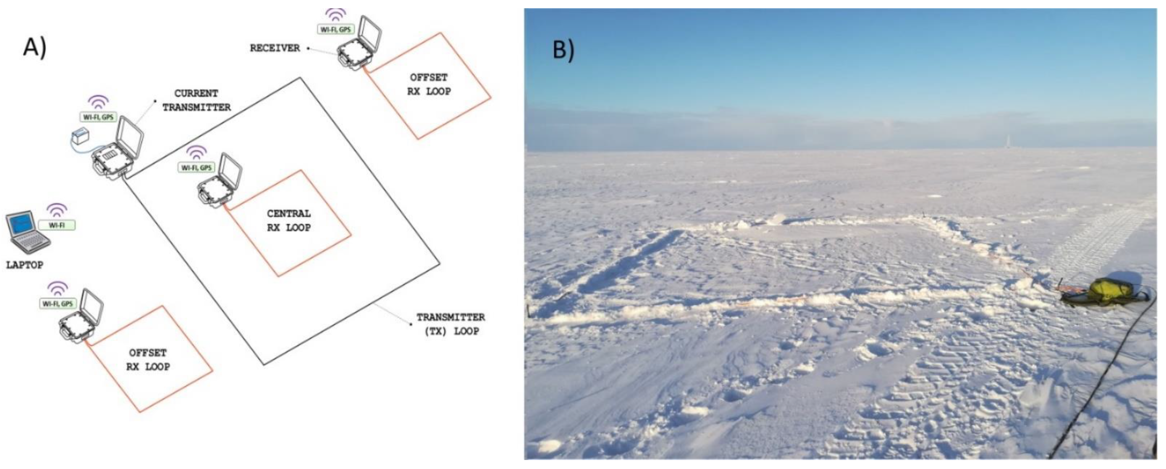
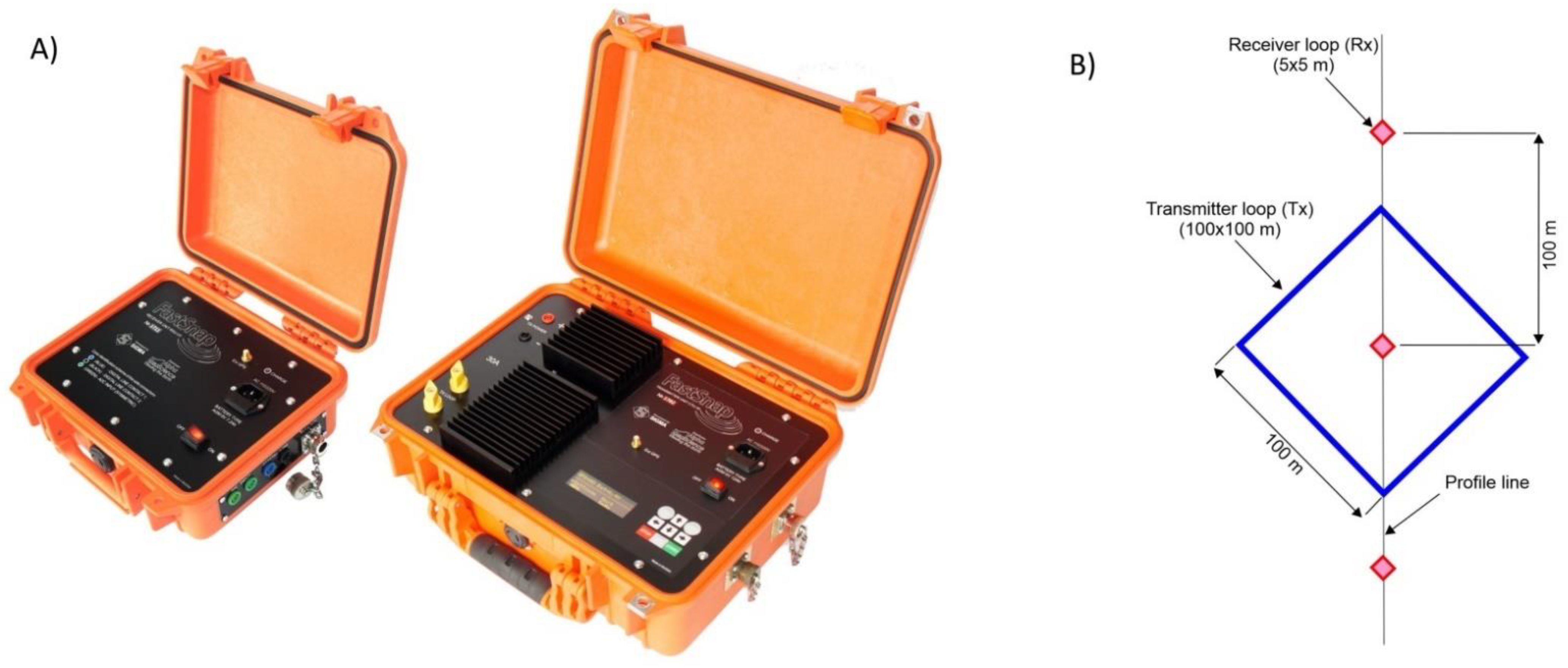
A large amount of sTEM soundings in Russia have been performed lately with a FastSnap multichannel digital telemeter system (Figure 1A and Figure 2A) [24] adapted to image complex resistivity patterns typical of Arctic regions. Surveys in shallow earth reach high performance at small transmitter loop sizes (less than 25 m × 25 m) and short transient times (<1 μs) [25]. The FastSnap system can run fast measurements of nanosecond times. The Arctic shallow earth is composed of resistive frozen rocks (permafrost) of hundreds or thousands of Ω·m. The presence of permafrost reduces the signal-to-noise (S/N) ratio and poses problems to measurements with small loops, as the recorded transients represent the frequency response of the loop more than the earth resistivity. Such loop effects on the signal have to be attenuated in a special way [26].

FastSnap can operate four receivers at a time. The multichannel telemetric architecture allows choosing survey design of any geometry, with the transmitter and receiver sizes and spacing tailored to specific objectives and required performance. The receiver units are connected to PC via digital transmitter lines (up to 400 m long) or using industrial-grade wireless connection, where possible, which makes the operation convenient and highly efficient. In the case of a three-channel system with Wi-Fi connection (Figure 1A), the transmitters are placed right near the receivers; the received signals are digitized and transmitted onto PC in a noise-immune form.

The operation of the FastSnap switch and the receivers is synchronized via GPS, to an error no worse than ±90 ns, or via a cable. The current switch is regulated by a built-in control or by the field laptop using special software. The current pulses can be of different polarities, with user-specified periods and intensities from 0.1 to 45 A. All units of the system are equipped with built-in GPS receivers that sample station coordinates and elevations.

The processing of the raw sTEM data and the inversion of transients are based on the integrated approach [27], with the use of diverse digital tools and the automatic correction of processing errors during the inversion. This approach ensures noise immunity and enhances the performance of the system in noisy urban or industrial environments. The correction improves the inversion quality and, in some cases, extends the imaged depth range, for instance, by attenuating the high-frequency ringing noise and reliable sampling of shallower earth.

The sTEM system, which is most often used for sounding to a depth of 500 m, comprises a 100 m × 100 m transmitter loop and three multicoil receivers (Figure 2B).

2.3. Survey Design

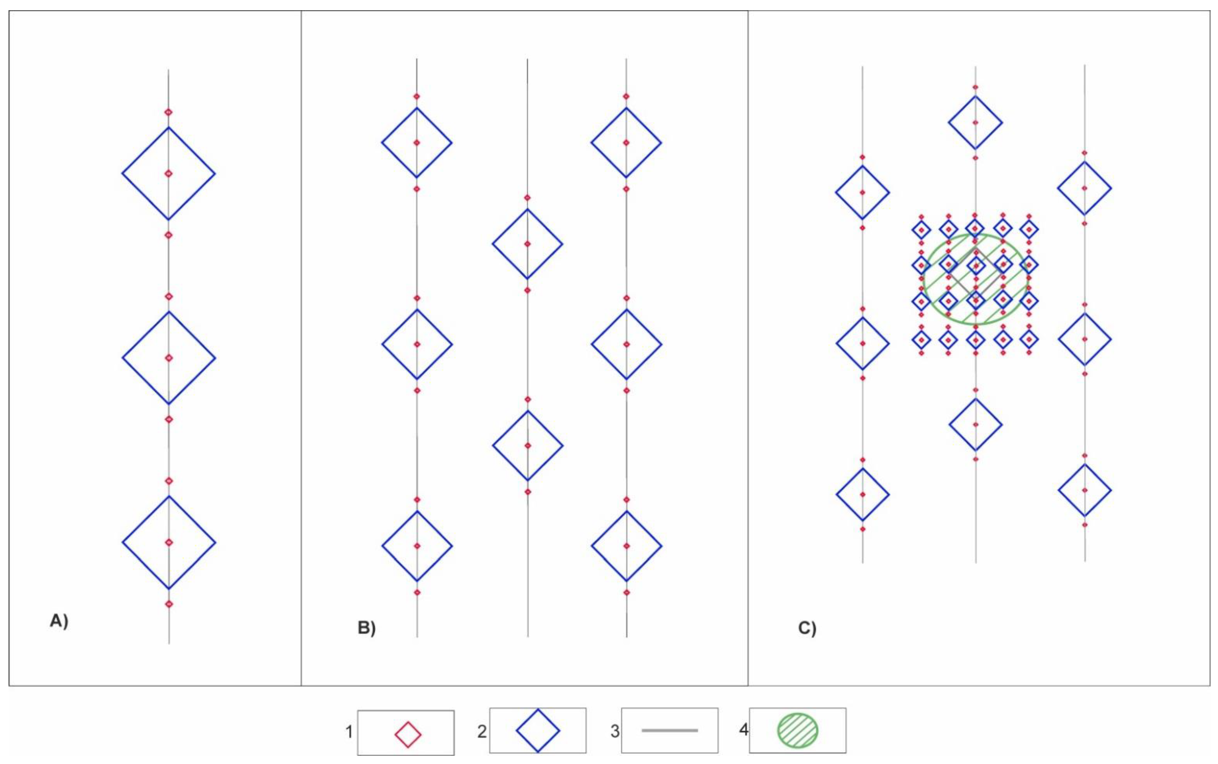
TEM stations can be placed along profiles (2D surveys) or on 2D arrays (3D surveys). Profile surveys are run mainly in urban areas or in areas not covered with seismic profiles, while 3D surveys provide high-resolution mapping of the near-surface and can follow the existing seismic networks; the sampling density can reach 16 to 33 points per km². High-density 3D data can be presented in the SEG-Y format suitable for joint interpretation of TEM and seismic measurements in the same modeling systems.

Properly choosing the geometry and array type is important to trade-off between information value, data quality, and operation costs. The choice stems from

• Subsurface (permafrost, taliks, cryopegs, resistivity contrasts, etc.) and surface (terrain) features;
• Required depth and lateral resolution;
• Absence/presence of seismic profiles, transmission lines, pipelines, or other infrastructure.

Subsurface features. In the last decade, the sTEM survey design in permafrost areas has been adapted to map the permafrost base, to contour taliks and cryopegs, and to detect faults and other zones of mechanic weakness. Before the field surveys in the Yamal-Nenets Autonomous District, the feasibility and potential performance of the chosen survey design was checked by forward modeling. The model included a 100 m × 100 m transmitter loop and receivers spaced at 100 m (Figure 2B), a design which has been tested largely for the past five years (>100,000 measurements) and was approved as a standard for such physiographic conditions.

Depth and lateral resolution. The chosen array geometry provides 500 m penetration, sufficient for imaging the resistivity patterns of permafrost. Spacing is set depending on the required lateral resolution; 100 m spacing is the most suitable for profiles to ensure high sampling density.

Infrastructure. The Arctic tundra landscapes, with flat terrain and poor vegetation, impose almost no limitations on the survey design and are thus favorable for sTEM soundings in any season. However, the petroleum production infrastructure can interfere with data quality, and careful choice of offset is required.

The receiver spacing for high-density 3D surveys (16 to 33 points per km²) can be slightly larger than in profile surveys (100 and 300 m or 100 and 400 m) in order to optimize the amount of measurements, often in the presence of 3D seismic networks.

The sTEM surveys, with the FastSnap systems and Wi-Fi data transmission, can be configured in any way, with greater sampling density at some local targets, e.g., at frost heaves (pingoes). Smaller loops are applied to shallowest features, below 2–3 m deep.

Thus, the sTEM method has demonstrated high performance and reliability in the Arctic areas of West Siberia, where more than 4000 km² of 3D data have been collected, at a penetration depth of 500 m. The resistivity patterns obtained with various survey designs (Figure 3) represent the permafrost structure, taliks, cryopegs, and faults.

3. Resistivity Patterns of Permafrost in Arctic Region

The near-surface geological model for Arctic areas may include intercalated sand and clay of Quaternary and Paleogene (Paleocene, Eocene, and Oligocene) ages. The sediments are perennially frozen in the upper few hundreds of meters.

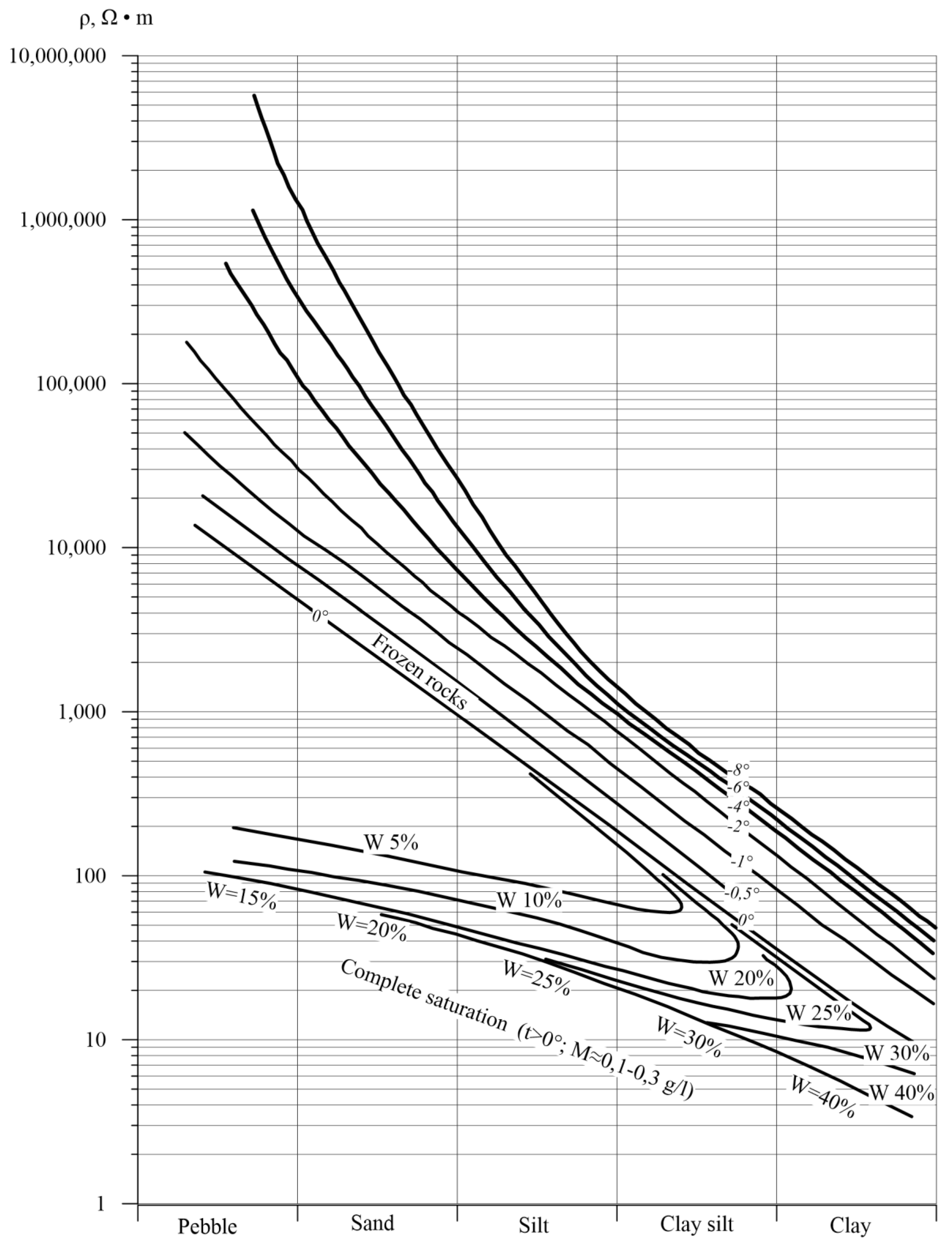
Phase changes of pore moisture (water-to-ice transition) are critical in terms of resistivity. Pure ice is conductive, but sediments are never 100% frozen, even in areas of thick permafrost. They contain unfrozen capillary moisture and are additionally saturated with saline water expulsed from freezing rocks. The amount of bound unfrozen pore water reduces as the temperatures become more negative and depends strongly on rock texture (pore space geometry). Bound water freezes up completely at temperatures below −50 °C, which rarely occurs in nature. On the other hand, the effect of interstitial ice on resistivity depends on its distribution in the pore space: rocks with massive cryostructure and conductive “bridges” between particles are moderately resistive and those with lens-like cryostructure (ice occupying most of the pore space) approach the resistivity of ice [6].

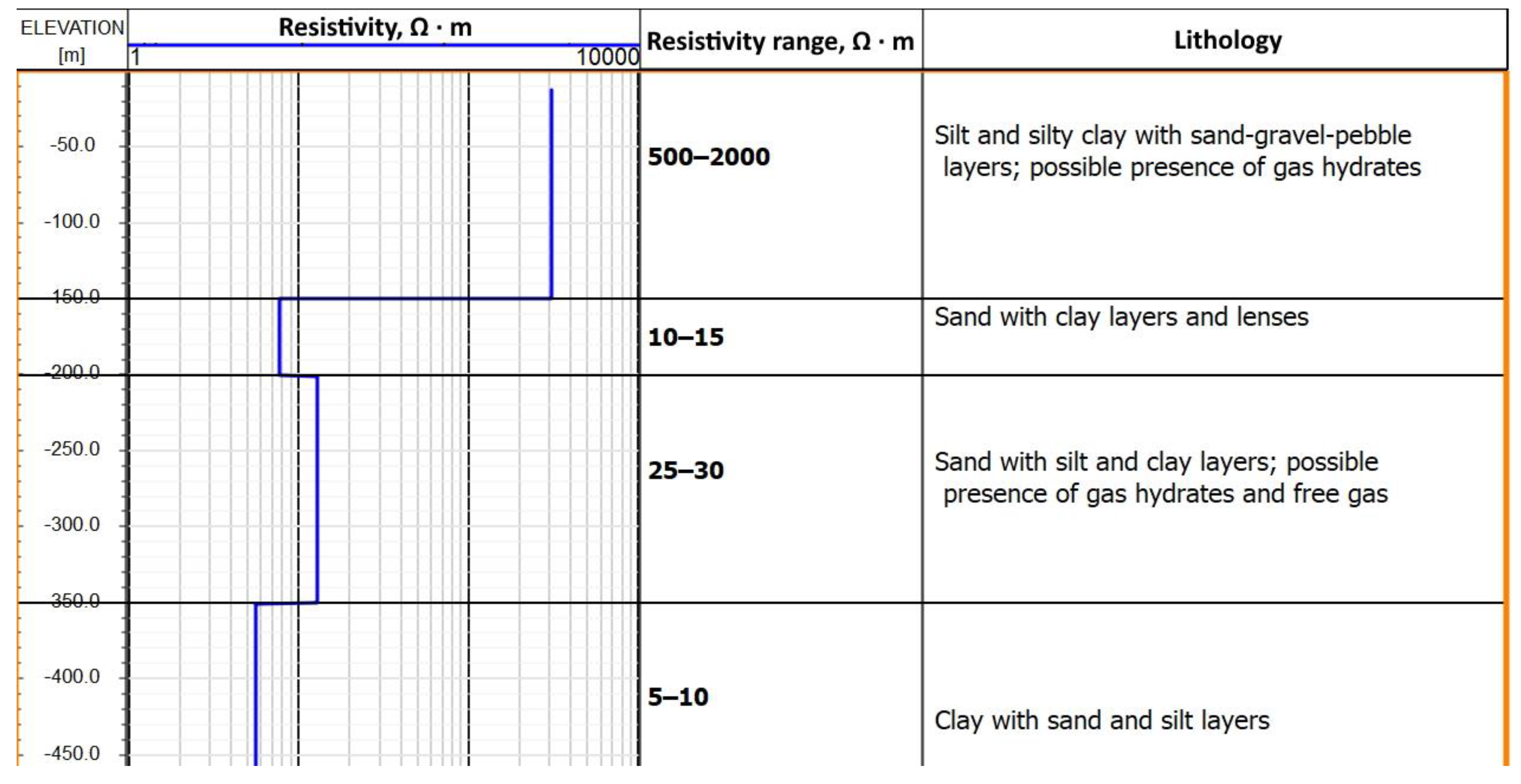
The resistivity of modern ice-rich permafrost reaches hundreds and thousands of Ω·m [28], but it is low (<10 Ω·m) in lenses of unfrozen saline water (cryopegs) and unfrozen rocks (taliks) inside and below permafrost. The resistivity of the Tabei–Sale formation, which is sometimes considered as corresponding to the permafrost base, is 30 Ω·m (Figure 4).

The high-resistivity frozen rocks stand out against conductive Mesozoic–Cenozoic sediments of the West Siberian basin.

At negative ground temperatures, free water converts to ice, and electric conduction is along films of unfrozen (mainly bound) water around mineral and ice particles. The presence of pore ice as a solid component changes the electric properties of rocks, which vary broadly depending on lithology, saturation, cryostructure, etc., as well as on various interactions between unfrozen water, the mineral matrix, and interstitial ice (Figure 5) [29].

Thus, the lithologically diverse shallow subsurface in the Arctic, with ice-rich permafrost and zones of unfrozen interstitial water, has a heterogeneous resistivity structure and thus lends itself to induction (TEM) surveys.

4. Results and Discussion

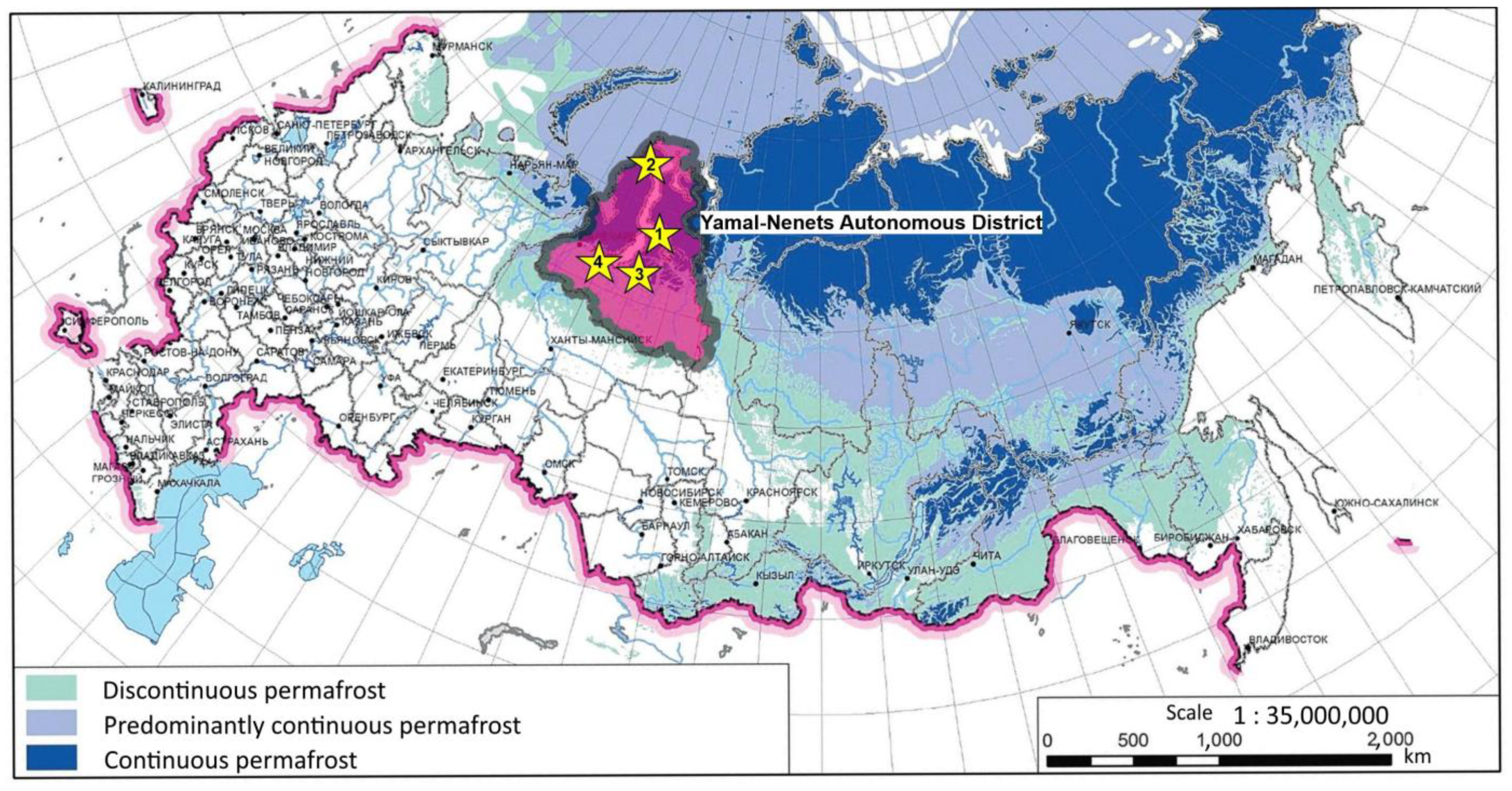
The sTEM soundings in the Russian Arctic have been conducted since 2016. The reported typical voltage decay curves (transient responses) were obtained from the northern Yamal Peninsula, southern Ob Gulf, and Nadym and Urengoi areas of the Yamal-Nenets Autonomous District (Figure 6). The acquisition was with 100 m × 100 m transmitter loops, 5 m × 5 m receiver loops, 0 and 100 m offsets, and 30 A maximum transmitter current.

The sTEM records of small square loops (<1000 m) often bear the effects of induced polarization (IP) [31,32,33,34,35,36,37,38,39,40,41]. The IP field outside the transmitter loop is much lower than in its center. On the other hand, central–loop signals from polarizable earth decay faster at later times than in the case of loop–loop data [20,21,42].

The known IP patterns can be included in forward solutions used as starting models for the inversion of multioffset data. Fast-decaying IP is described using the Cole–Cole complex frequency-dependent conductivity related to the chargeability, relaxation time, and exponent (referring to spectral shape) [43,44,45].

The transients obtained with loop–loop arrays are less affected by induced polarization, and the respective starting models (layer thicknesses and resistivities) are used for reference in the inversion of central–loop data. At the next step, the computed model is fitted to observations to find the IP parameters that provide the minimum misfit (minimizing the misfit functional). Thus, the inversion of TEM data yields reliable resistivity patterns of polarizable earth.

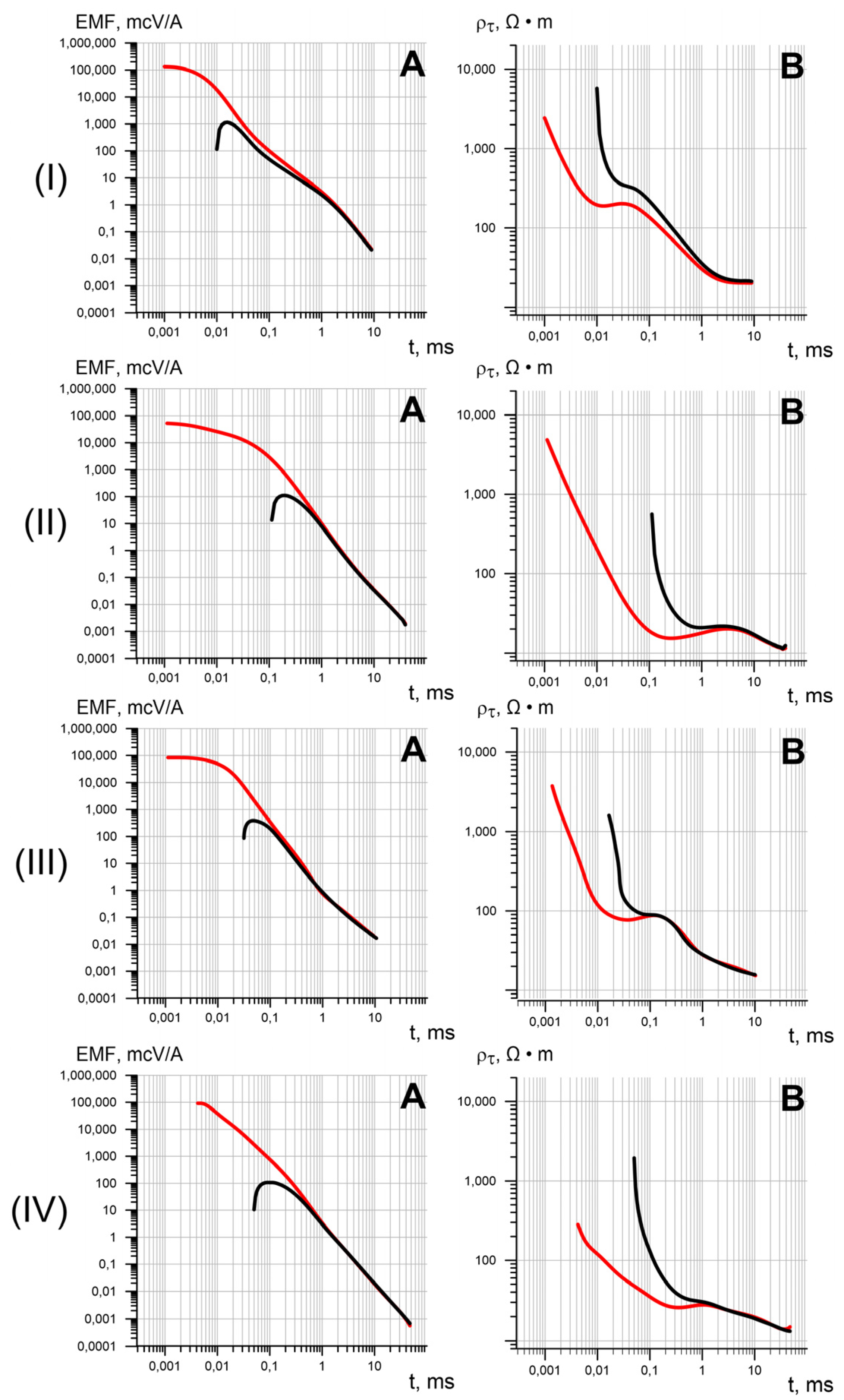
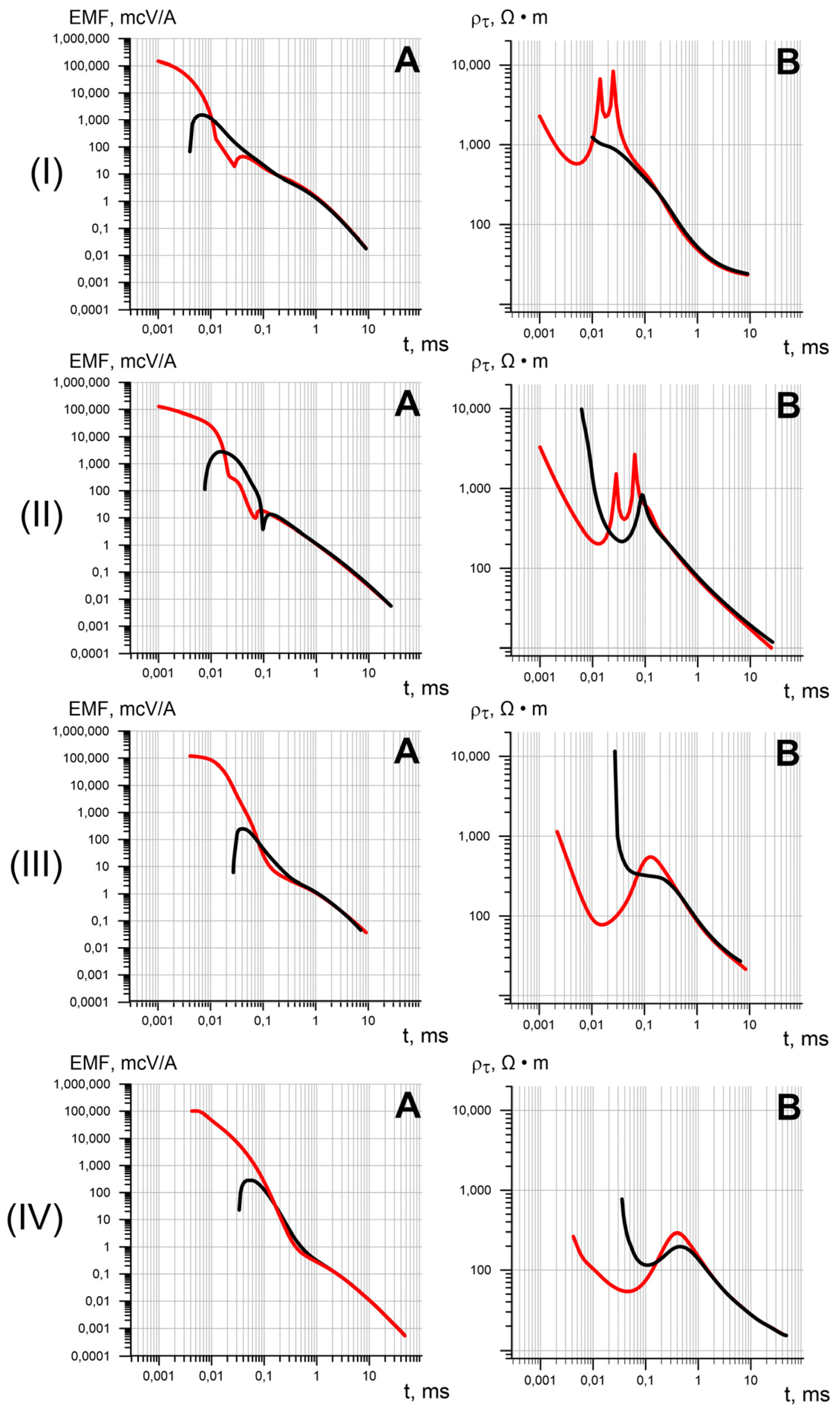
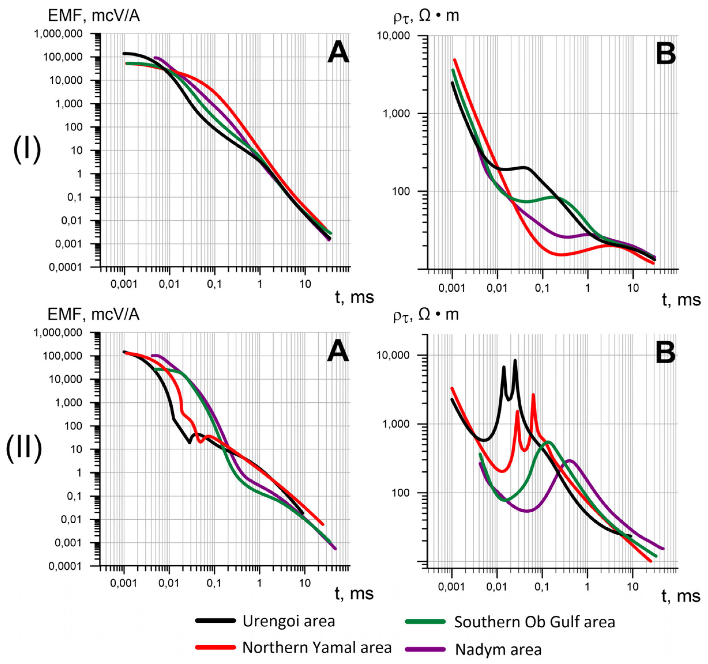
For more correct comparison, the field sTEM data were divided into two groups: affected by IP (Figure 7) and free from IP effects (Figure 8). In the Urengoi area (Figure 7I), the transient process (voltage decay) lasts 10 ms and the minimum apparent resistivities are 200 Ω·m at 3 ms and 20 Ω·m at 0.01 ms (Figure 7I(A,B)). The left branch of the curves represents frozen earth, while the segment at t > 1–2 ms corresponds to low-temperature but ice-free rocks with apparent resistivity of ~20 Ω·m, below the level of the resistive ice-rich permafrost.

The responses acquired with the central–loop system (Figure 8I,II(A,B)) show sign reversal associated with IP effects at the times between 0.01 and 0.1 ms. Later than 0.1 ms, the curves of the central–loop and loop–loop arrays match well, and the voltage decay stops at a resistivity of 10–20 Ω·m.

The sTEM responses from the northern Yamal Peninsula (Figure 7II) have a longer transient time (Figure 7II(A)) of 40 ms, with apparent resistivity minimums (Figure 7II(B)) at 0.2 ms (17 Ω·m) and 30 ms (10 Ω·m); resistivity in the middle times is ~20 Ω·m.

The IP effects in the central–loop data (Figure 8II(A)) produce a resistivity anomaly at early times (0.01–0.1 ms). Sign reversal appears first at 0.03 ms and then at 0.07 ms. Meanwhile the loop–loop patterns are similar: the central–loop and loop–loop curves coincide after 0.2 ms, and the decay stops at 10–20 Ω·m.

The transient time and the minimum apparent resistivities in the sTEM data from the Nadym area (Figure 7III) are, respectively, 20 ms (Figure 7III(A)) and 90 Ω·m at 0.03 ms and 40 Ω·m at 0.5 ms (Figure 7III(B)). The descending branch of the curve represents low-temperature ice-free rocks at later times.

IP effects in the central–loop data (Figure 8III(B)) appear as a resistivity high of 500 Ω·m in the 0.05–0.3 ms interval. At the times later than 0.4 ms, the curves recorded by central–loop and loop–loop arrays coincide, and the end of the transient process corresponds to the apparent resistivity <20 Ω·m.

The curves from the southern Ob Gulf Figure 7IV show the 40 ms duration of the voltage decay (Figure 7IV(A)) and the apparent resistivity minimums (Figure 7IV(B)) at 0.005 ms (150 Ω·m) and 0.3 ms (25 Ω·m). The late-time resistivity decreases gradually to 15 Ω·m.

The data affected by the induced polarization (Figure 8IV(B)) reveal two resistivity lows of 150 Ω·m at 0.007 ms and 50 Ω·m 0.04 ms, as well as a 300 Ω·m high. The central–loop and loop–loop data coincide at >1.3 ms and the decay completes at 15 Ω·m.

The summarized four datasets (Figure 9) show that the sTEM curves free from IP effects collected in different areas of the Yamal-Nenets Autonomous District (Figure 9I) differ considerably only at early times before 1–2 ms and represent low-temperature ice-free rocks with low resistivity (15–20 Ω·m) at later times. The apparent resistivity is the highest (200 Ω·m) in the Urengoi area, at early times < 1 ms, moderate (a few tens of Ω·m) in the Nadym and southern Ob Gulf areas, and the lowest in the Northern Yamal Peninsula, where shallow sediments are saline. Near-surface aquifers (and related cryopegs) are saturated with saline water and remain unfrozen even within permafrost. The resistivity models (

Table 1. sTEM resistivity models.

Urengoi Area		Northern Yamal		Nadym Area		Southern Ob Gulf
ρ, Ω·m	H, m	ρ, Ω·m	H, m	ρ, Ω·m	H, m	ρ, Ω·m	H, m
2000	80	30	30	1500	180	50	20
700	25	50	10	40	30	1300	120
900	40	1000	130	5	20	600	40
2000	60	40	200	40	90	10	10
10	30			15	120	50	150
40	240			40	60	60	120

) based on the inversion of sTEM data predict low resistivity (30–50 Ω·m) in two upper layers corresponding to cryopegs.

The sTEM curves were inverted within the deterministic framework, with the thickness and resistivity of the model layers allowed to vary. The 1D Earth responses from each sounding point were first processed using the forward algorithm developed at the Trofimuk Institute of Petroleum Geology and Geophysics, Siberian Branch of the Russian Academy of Sciences (IPGG, Novosibirsk). The forward solution was obtained with regard to the durations of the current pulse and current turn-off (ramp). The inversion was carried out iteratively, adjusting the resistivity and layer thicknesses until the misfit between the theoretical and field curves reached the minimum. No limitations for changes in layer resistivity were imposed. During the inversion, the induced polarization parameters were taken into account as the Cole–Cole complex frequency-dependent conductivity related with the chargeability, relaxation time, and exponent. The average inversion misfit did not exceed 5%. The results of the sTEM inversion were checked against resistivity logs for the boundaries of geological intervals and sTEM resistivity patterns.

The sTEM responses of a polarizable earth from different areas (Figure 9II) have diverse shapes depending on the depths to polarization interfaces, relaxation times, and IP features. The chargeability varies from 0.1 to 0.7 and the relaxation time is from 6 × 10⁻⁵ to 1.5 × 10⁻⁴ s.

The inversion of the field sTEM data with regard to the induced polarization ensured high-quality resistivity models (Table 1) suitable for geological modeling.

The thickness of the ice-rich permafrost in the studied Arctic areas inferred from sTEM resistivity data mostly varies from 170 to 205 m and reaches 250 m in the model for the northern Yamal (Figure 10). The model images low-resistivity lenses in the permafrost, possibly associated with cryopegs.

The permafrost is continuous and 250 m thick in the western part of the area and is almost absent in the east, where the Ob Gulf is marked by a low resistivity of around 10 Ω·m. An open talik under the Saboliyakha River is marked by a resistivity low prominent against high-resistivity permafrost. The rocks below the permafrost base and deeper than 400 m are highly resistive, possibly in the presence of clathrate or free gas.

Thus, the sTEM soundings are applicable to study the permafrost structure and to map cryopegs, taliks, pingoes, and vertical faults in Arctic West Siberia [46,47,48,49,50].

5. Conclusions

This research was undertaken to test the efficiency of induction-based electromagnetic surveys in studies of permafrost and to find new evidence for the similarity and difference of the permafrost structure in different areas of Northern Siberia.

The results show that induction surveys, especially shallow transient electromagnetic soundings, offer a good tool to image the shallow subsurface of the Arctic region dominated by permafrost. According to our field experience for the past five years, the sTEM measurements, which can run in any season and in any climate conditions, to a depth of 500 m, are advantageous in this respect. The induction surveys are well suitable for imaging the frozen shallow subsurface because they require no galvanic contact with the earth and no grounding.

The sTEM curves were collected in the Urengoi, Nadym, Southern Ob Gulf, and Northern Yamal areas of Northern Siberia, which have different permafrost settings. The collected sTEM data were divided into two groups according to the presence or absence of IP effects. The TEM data affected by IP were inverted using the Cole–Cole complex frequency-dependent conductivity related to the chargeability, relaxation time, and exponent. The collected earth responses were processed using advanced tools to provide geologically essential information from late-time records, while optimized inversion algorithms were applied to obtain high-quality layered resistivity models.

The resulting geoelectric models from the four areas showed obvious differences in the thickness of highly resistive frozen rocks and the location of unfrozen zones (taliks). The TEM-based resistivity patterns clearly resolve the permafrost base, as well as the contours of taliks, the lenses of saline water (cryopegs), gas hydrates, and frost-heaving features.

The TEM-based resistivity patterns reveal evident variations in the thickness of highly resistive frozen rocks and the presence of unfrozen patches. They clearly resolve the permafrost base, as well as the contours of unfrozen zones (taliks), the lenses of saline water (cryopegs), gas hydrates, and frost-heaving features.

The reported results can be used to choose geophysical methods best suitable for permafrost studies in the harsh Arctic conditions. Furthermore, the presented resistivity patterns can make reference for future studies of permafrost in Northern Siberia.

The complex structure of the Arctic permafrost and subpermafrost layers should be studied jointly by several geophysical methods: sTEM, shallow seismic, radar, and ERT surveys. It is essential to check the TEM-based resistivity images against the resistivity, temperature, and other well logs for more precise correlation between the resistivity and lithology variations, and for high-quality permafrost imaging.

Further research in this line is required to provide new insights into the local geology, as well as into processes in the permafrost, which are essential elements of the fragile Arctic ecosystem.