
Numerical Study and Force Chain Network Analysis of Sand Production Process Using Coupled LBM-DEM


Abstract
:1. Introduction
2. Methodology
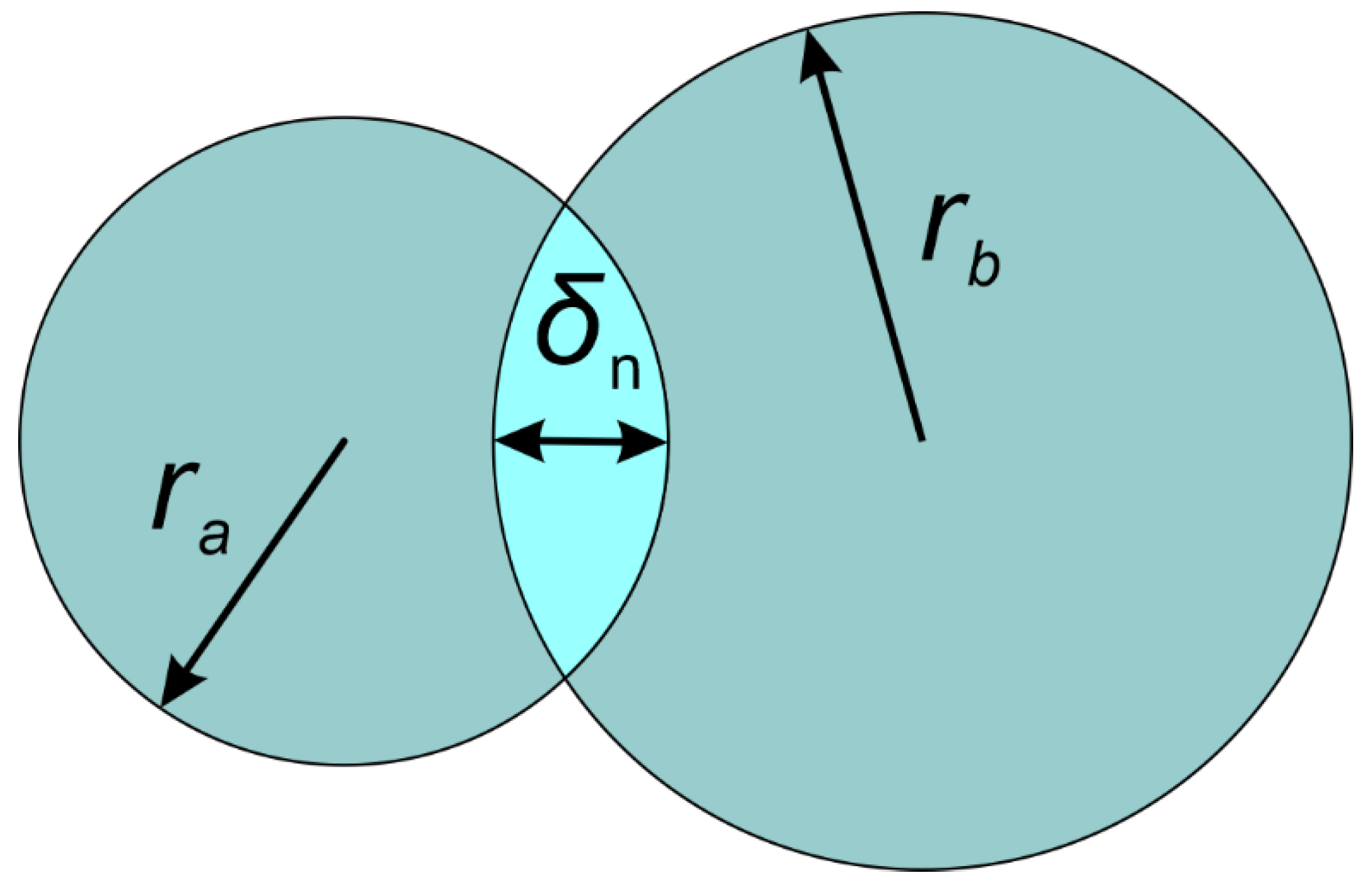
2.1. Bonded DEM
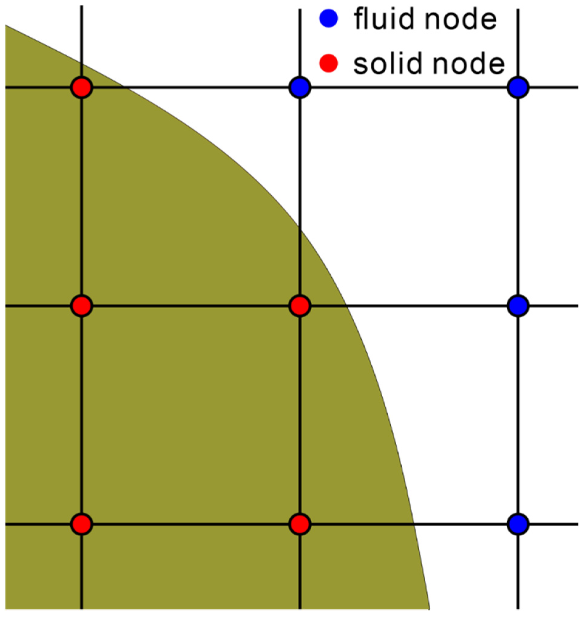
2.2. Lattice Boltzmann Method
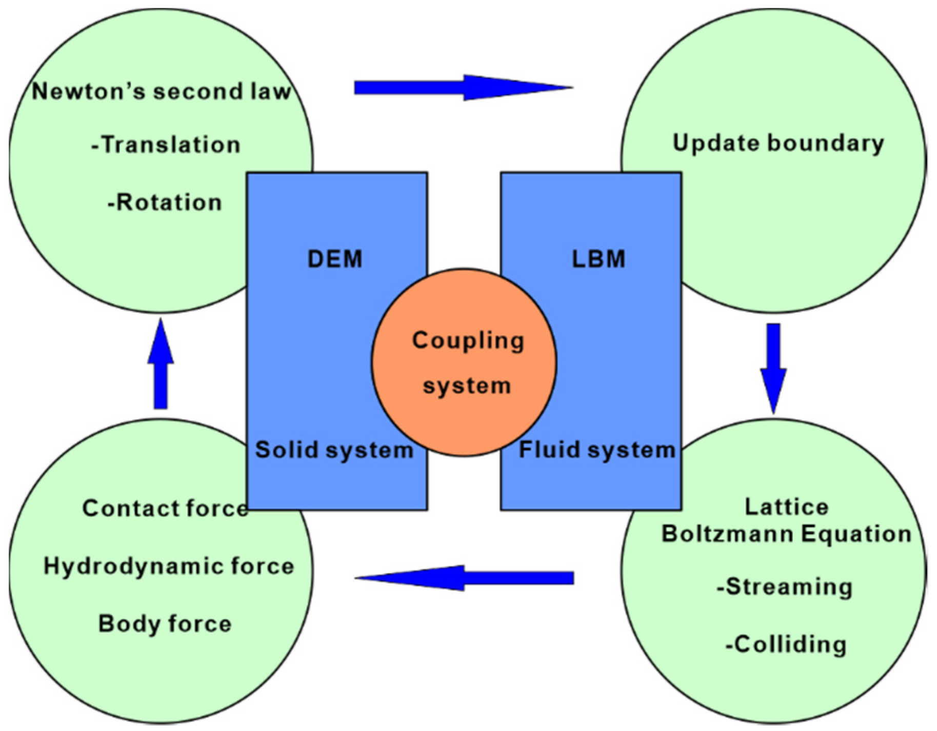
2.3. LBM-DEM Coupling
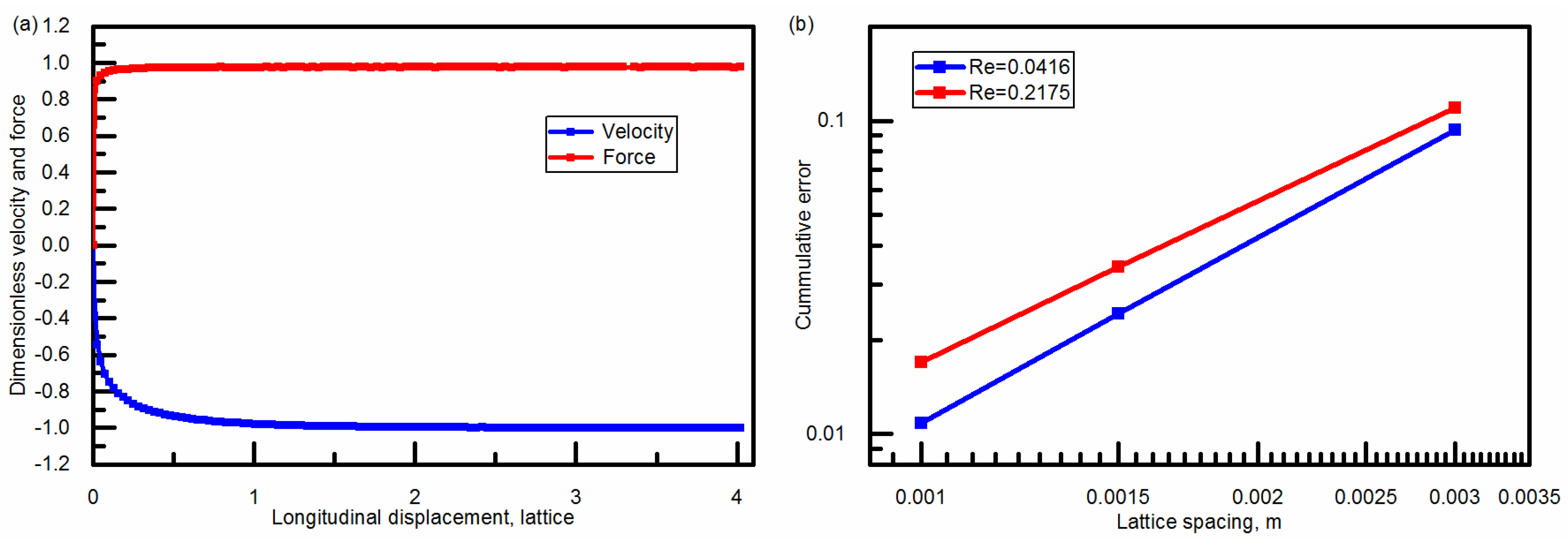
2.4. Method Validation
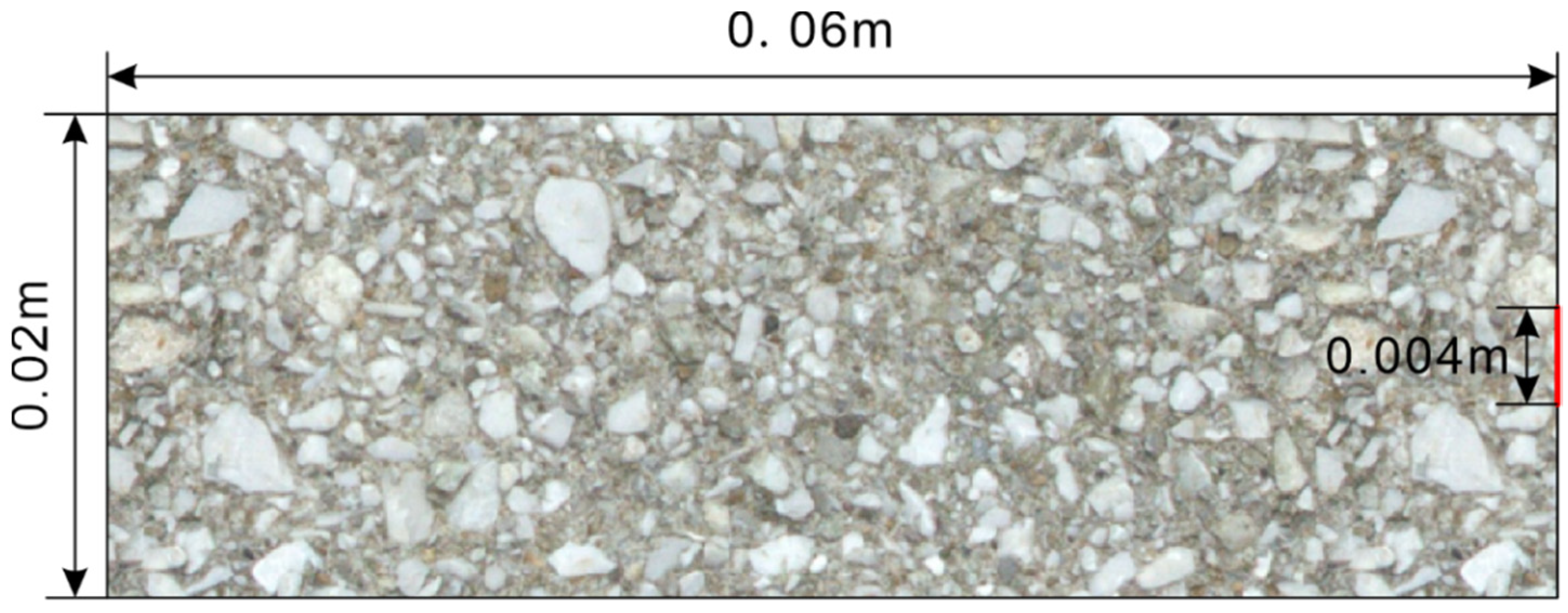
2.5. Model Setup
3. Results and Discussion
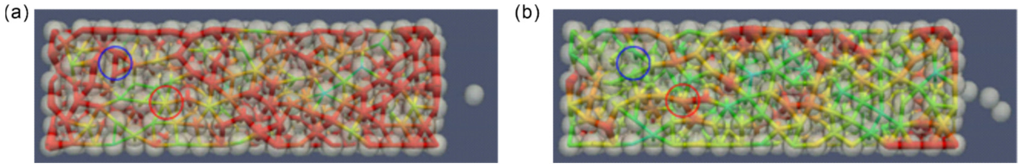
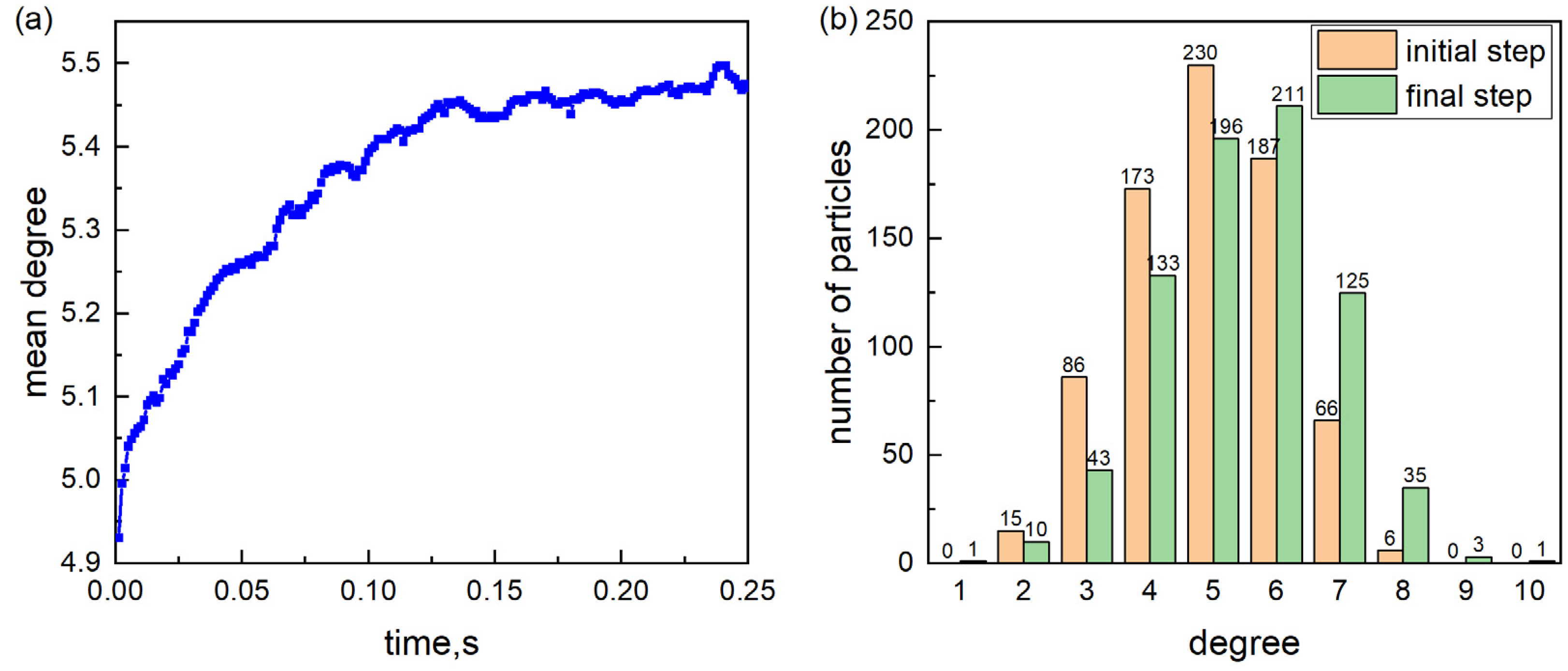
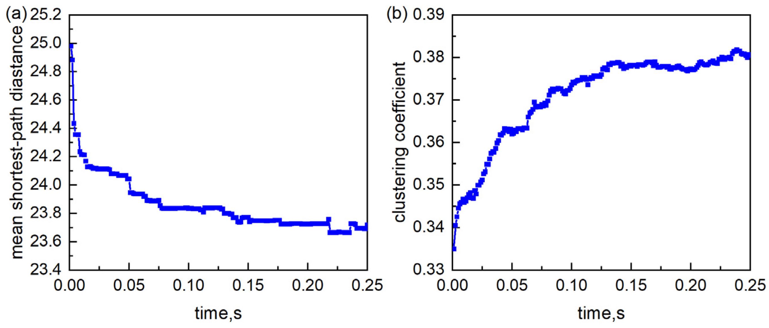
3.1. Force Chain Network Analysis
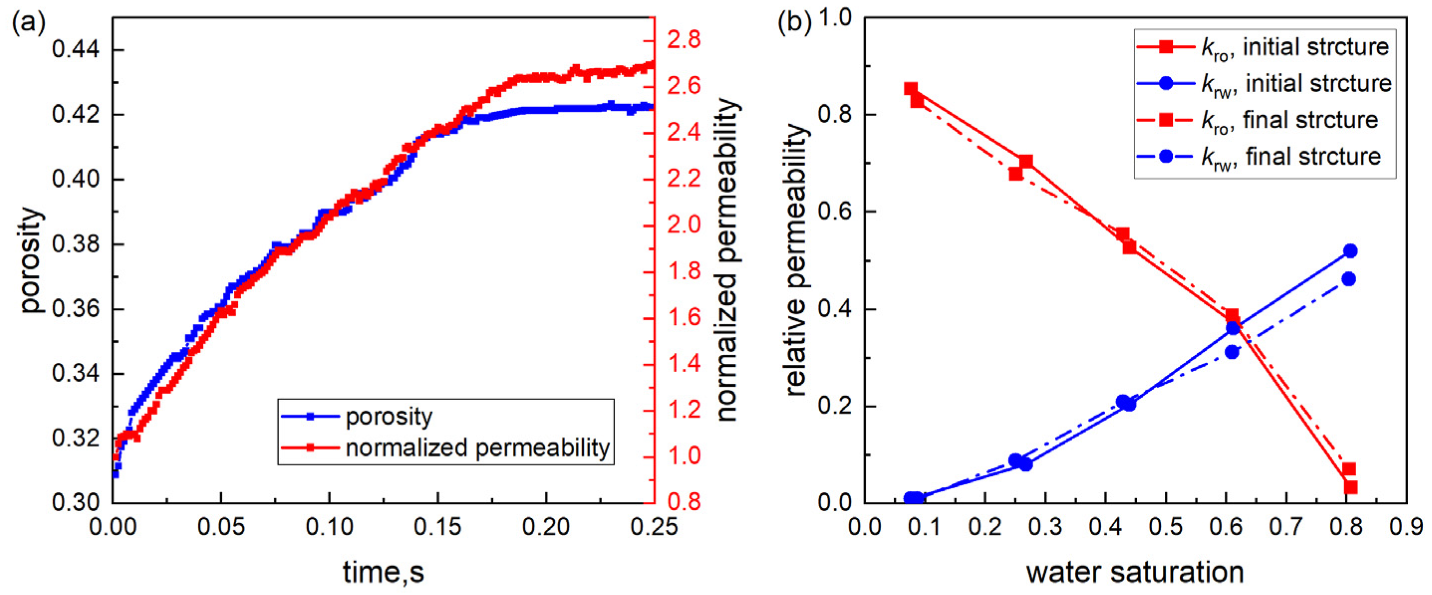
3.2. Absolute Permeability and Relative Permeability
3.3. The Effect of Injection Flow Rate
3.4. The Effect of Cementation Strength
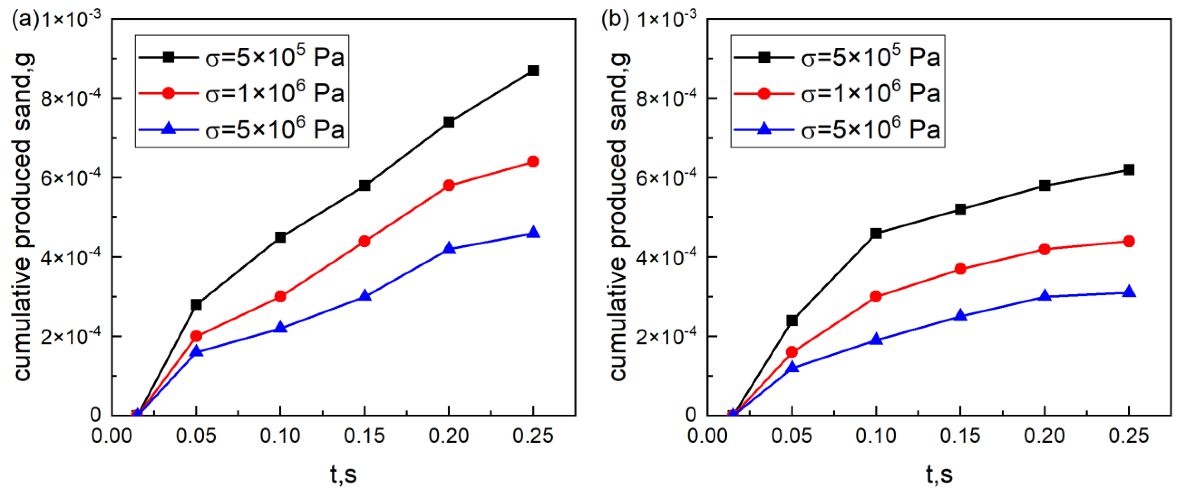
3.5. The Effect of Confining Pressure
4. Conclusions
Author Contributions
Funding
Institutional Review Board Statement
Informed Consent Statement
Data Availability Statement
Conflicts of Interest
Nomenclature
| Symbols | |
| m | particle mass, kg |
| v | particle velocity, m/s |
| t | time, s |
| Fb | body force, N |
| Fc | contact force, N |
| Fh | hydrodynamic force, N |
| I | particle inertia, kg·m2 |
| Tc | torque generated by the contact force, N·m |
| Th | hydrodynamic torque, N·m |
| kn | normal stiffness, kg/m2 |
| Fmax | critical tensile force, N |
| x | position in the lattice space, lu (lattice unit) |
| ea | directional lattice velocity, lu/ts |
| f | particle distribution function, dimensionless |
| feq | equilibrium distribution function, dimensionless |
| a | discretized direction, dimensionless |
| c | basic speed on the lattice, lu/ts |
| u | macroscopic velocity, m/s |
| cs | lattice sound velocity, lu/ts |
| p | pressure, Pa |
| bounce-back of the non-equilibrium part of the distribution function, dimensionless | |
| Ff | fluid-fluid interaction force, N |
| Fads | fluid-solid interaction force, N |
| r | particle radius, m |
| l | distance between the particle center and the wall, m |
| Re | Reynold number, dimensionless |
| E | elastic modulus, Pa |
| fr | coefficient of surface friction, dimensionless |
| Fsim | force calculated by the simulaiton method, N |
| Fa | force calculated by the analytical method, N |
| de | degree of the node, dimensionless |
| L | mean shortest-path distance, dimensionless |
| C | global clustering coefficient, dimensionless |
| k | permeability, μm2 |
| Q | flow rate, m3/s |
| Greek Letters | |
| ω | particle angular velocity, rad/s |
| η | Poisson’s ratio of the particle, dimensionless |
| δn | overlapping length, m |
| τ | collision relaxation time, dimensionless |
| Δt | time interval, ts (time step) |
| Δx | lattice spacing, lu |
| ν | kinetic viscosity, m2/s |
| ρ | fluid density, kg/m3 |
| ρs | particle density, kg/m3 |
| γ | solid fraction of a cell, dimensionless |
| β | weighting function, dimensionless |
| ε | cumulative error, dimensionless |
| σ | cementation strength, Pa |
| Subscripts | |
| b | body |
| c | contact |
| h | hydrodynamic |
| a | the ath |
| σ | the σth |
| i | the ith |
| j | the jth |
| Superscripts | |
| eq | the equilibrium state |
| σ | the σth |
| n | the n step |
References
- Walton, I.C.; Atwood, D.C.; Halleck, P.M.; Bianco, L.C. Perforating unconsolidated sands: An experimental and theoretical investigation. In Proceedings of the SPE Annual Technical Conference and Exhibition, New Orleans, LA, USA, 30 September–3 October 2001. [Google Scholar]
- Bianco, L.; Halleck, P. Mechanisms of arch instability and sand production in two-phase saturated poorly consolidated sandstones. In Proceedings of the SPE European Formation Damage Conference, The Hague, The Netherlands, 21–22 May 2001. [Google Scholar]
- Xia, T.; Feng, Q.; Wang, S.; Zhao, Y.; Xing, X. A Bonded 3D LBM-DEM Approach for Sand Production Process. In Proceedings of the SPE Asia Pacific Oil & Gas Conference and Exhibition, Virtual, 17–19 November 2020. [Google Scholar]
- Terzaghi, K. Stress distribution in dry and in saturated sand above a yielding trap-door. In Proceedings of the International Conference on Soil Mechanics, Cambridge, MA, USA, 22–26 June 1936. [Google Scholar]
- Hall, C.; Harrisberger, W. Stability of sand arches: A key to sand control. J. Pet. Technol. 1970, 22, 821–829. [Google Scholar] [CrossRef]
- Clearly, M.P.; Melvan, J.J.; Kohlhaas, C.A. The effect of confining stress and fluid properties on arch stability in unconsolidated sands. In Proceedings of the SPE Annual Technical Conference and Exhibition, Las Vegas, NV, USA, 23–26 September 1979. [Google Scholar]
- Cook, J.; Bradford, I.; Plumb, R. A study of the physical mechanisms of sanding and application to sand production prediction. In Proceedings of the European Petroleum Conference, London, UK, 25–27 October 1994. [Google Scholar]
- Yim, K.; Dusseault, M.; Zhang, L. Experimental study of sand production processes near an orifice. In Proceedings of the Rock Mechanics in Petroleum Engineering, Delft, The Netherlands, 29–31 August 1994. [Google Scholar]
- Geilikman, M.; Dusseault, M.; Dullien, F. Sand production as a viscoplastic granular flow. In Proceedings of the SPE formation damage control symposium, Lafayette, LA, USA, 7–10 February 1994. [Google Scholar]
- Bratli, R.K.; Risnes, R. Stability and failure of sand arches. Soc. Pet. Eng. J. 1981, 21, 236–248. [Google Scholar] [CrossRef]
- Vardoulakis, I.; Stavropoulou, M.; Papanastasiou, P. Hydro-mechanical aspects of the sand production problem. Transp. Porous Media 1996, 22, 225–244. [Google Scholar] [CrossRef]
- Papamichos, E.; Vardoulakis, I.; Tronvoll, J.; Skjaerstein, A. Volumetric sand production model and experiment. Int. J. Numer. Anal. Methods Geomech. 2001, 25, 789–808. [Google Scholar] [CrossRef]
- Isehunwa, O.; Farotade, A. Sand failure mechanism and sanding parameters in Niger Delta oil reservoirs. Int. J. Eng. Sci. Tecnol. 2010, 2, 777–782. [Google Scholar]
- Detournay, C.; Wu, B.; Cotthem, A.; Charlier, R.; Thimus, J. Semi-analytical models for predicting the amount and rate of sand production. In EUROCK 2006: Multiphysics Coupling and Long Term Behaviour in Rock Mechanics; Taylor & Francis Group: London, UK, 2006; pp. 373–380. [Google Scholar]
- OConnor, R.i.M.; Torczynski, J.R.; Preece, D.S.; Klosek, J.T.; Williams, J.R. Discrete element modeling of sand production. Int. J. Rock Mech. Min. Sci. Geomech. Abstr. 1997, 34, 231.e1–231.e15. [Google Scholar] [CrossRef]
- Jensen, R.P.; Preece, D.S. Modeling sand Production with Darcy-Flow Coupled with Discrete Elements; Sandia National Labs.: Albuquerque, NM, USA, 2000. [Google Scholar]
- Li, L.; Papamichos, E.; Cerasi, P. Investigation of sand production mechanisms using DEM with fluid flow. Multiphysics Coupling Long Term Behav. Rock Mech. 2006, 1, 241–247. [Google Scholar]
- Han, Y.; Cundall, P.A. LBM–DEM modeling of fluid–solid interaction in porous media. Int. J. Numer. Anal. Methods Geomech. 2013, 37, 1391–1407. [Google Scholar] [CrossRef]
- Kefayati, G. Lattice Boltzmann simulation of double-diffusive natural convection of viscoplastic fluids in a porous cavity. Phys. Fluids 2019, 31, 013105. [Google Scholar] [CrossRef]
- Kefayati, G.; Tolooiyan, A.; Bassom, A.P.; Vafai, K. A mesoscopic model for thermal–solutal problems of power-law fluids through porous media. Phys. Fluids 2021, 33, 033114. [Google Scholar] [CrossRef]
- Kefayati, G.R. Thermosolutal natural convection of viscoplastic fluids in an open porous cavity. Int. J. Heat Mass Transf. 2019, 138, 401–419. [Google Scholar] [CrossRef]
- Kefayati, G.R.; Tang, H.; Chan, A.; Wang, X. A lattice Boltzmann model for thermal non-Newtonian fluid flows through porous media. Comput. Fluids 2018, 176, 226–244. [Google Scholar] [CrossRef]
- Cook, B.K.; Noble, D.R.; Williams, J.R. A direct simulation method for particle-fluid systems. Eng. Comput. 2004, 21, 151–168. [Google Scholar] [CrossRef]
- Boutt, D.F.; Cook, B.K.; McPherson, B.J.; Williams, J. Direct simulation of fluid-solid mechanics in porous media using the discrete element and lattice-Boltzmann methods. J. Geophys. Res. Solid Earth 2007, 112, 1978–2012. [Google Scholar] [CrossRef] [Green Version]
- Feng, Y.T.; Han, K.; Owen, D.R.J. Coupled lattice Boltzmann method and discrete element modelling of particle transport in turbulent fluid flows: Computational issues. Int. J. Numer. Methods Eng. 2007, 72, 1111–1134. [Google Scholar] [CrossRef]
- Han, K.; Feng, Y.T.; Owen, D.R.J. Coupled lattice Boltzmann and discrete element modelling of fluid–particle interaction problems. Comput. Struct. 2007, 85, 1080–1088. [Google Scholar] [CrossRef]
- Han, K.; Feng, Y.T.; Owen, D.R.J. Numerical simulations of irregular particle transport in turbulent flows using coupled LBM-DEM. Cmes-Comp. Model. Eng. 2007, 18, 87–100. [Google Scholar]
- Cundall, P.A.; Strack, O.D. A discrete numerical model for granular assemblies. Geotechnique 1979, 29, 47–65. [Google Scholar] [CrossRef]
- Potyondy, D.O.; Cundall, P. A bonded-particle model for rock. Int. J. Rock Mech. Min. Sci. 2004, 41, 1329–1364. [Google Scholar] [CrossRef]
- Cundall, P.; Strack, O. Particle Flow Code in 2 Dimensions; Itasca Consulting Group, Inc.: Minneapolis, MN, USA, 1999. [Google Scholar]
- Wang, M.; Feng, Y.; Wang, C. Coupled bonded particle and lattice Boltzmann method for modelling fluid–solid interaction. Int. J. Numer. Anal. Methods Geomech. 2016, 40, 1383–1401. [Google Scholar] [CrossRef]
- Utili, S.; Nova, R. DEM analysis of bonded granular geomaterials. Int. J. Numer. Anal. Methods Geomech. 2008, 32, 1997–2031. [Google Scholar] [CrossRef]
- Wang, Y.; Leung, S. Characterization of cemented sand by experimental and numerical investigations. J. Geotech. Geoenviron. Eng. 2008, 134, 992–1004. [Google Scholar] [CrossRef]
- Obermayr, M.; Dressler, K.; Vrettos, C.; Eberhard, P. A bonded-particle model for cemented sand. Comput. Geotech. 2013, 49, 299–313. [Google Scholar] [CrossRef]
- Eshghinejadfard, A.; Daróczy, L.; Janiga, G.; Thévenin, D. Calculation of the permeability in porous media using the lattice Boltzmann method. Int. J. Heat Fluid Flow 2016, 62, 93–103. [Google Scholar] [CrossRef]
- Wang, M.; Feng, Y.; Wang, C. Numerical investigation of initiation and propagation of hydraulic fracture using the coupled Bonded Particle–Lattice Boltzmann Method. Comput. Struct. 2017, 181, 32–40. [Google Scholar] [CrossRef]
- Timm, K.; Kusumaatmaja, H.; Kuzmin, A.; Shardt, O.; Silva, G.; Viggen, E. The Lattice Boltzmann Method: Principles and Practice; Springer International Publishing: Cham, Switzerland, 2016. [Google Scholar]
- Shan, X.; Chen, H. Lattice Boltzmann model for simulating flows with multiple phases and components. Phys. Rev. E 1993, 47, 1815. [Google Scholar] [CrossRef] [Green Version]
- Ladd, A.; Verberg, R. Lattice-Boltzmann simulations of particle-fluid suspensions. J. Stat. Phys. 2001, 104, 1191–1251. [Google Scholar] [CrossRef]
- Buick, J.; Greated, C. Gravity in a lattice Boltzmann model. Phys. Rev. E 2000, 61, 5307. [Google Scholar] [CrossRef] [Green Version]
- Guo, Z.; Zheng, C.; Shi, B. Discrete lattice effects on the forcing term in the lattice Boltzmann method. Phys. Rev. E 2002, 65, 046308. [Google Scholar] [CrossRef]
- Kupershtokh, A.; Medvedev, D.; Karpov, D. On equations of state in a lattice Boltzmann method. Comput. Math. Appl. 2009, 58, 965–974. [Google Scholar] [CrossRef] [Green Version]
- Sukop, M.; Thorne, D. Lattice Boltzmann Modeling: An Introduction for Geoscientists and Engineers; Springer: Berlin, Germany, 2005. [Google Scholar]
- Landry, C.; Karpyn, Z.; Ayala, O. Relative permeability of homogenous-wet and mixed-wet porous media as determined by pore-scale lattice Boltzmann modeling. Water Resour. Res. 2014, 50, 3672–3689. [Google Scholar] [CrossRef] [Green Version]
- Sega, M.; Sbragaglia, M.; Kantorovich, S.S.; Ivanov, A.O. Mesoscale structures at complex fluid–fluid interfaces: A novel lattice Boltzmann/molecular dynamics coupling. Soft Matter 2013, 9, 10092–10107. [Google Scholar] [CrossRef] [Green Version]
- Shan, X.; Doolen, G. Multicomponent lattice-Boltzmann model with interparticle interaction. J. Stat. Phys. 1995, 81, 379–393. [Google Scholar] [CrossRef] [Green Version]
- Noble, D.; Torczynski, J. A lattice-Boltzmann method for partially saturated computational cells. Int. J. Mod. Phys. C 1998, 9, 1189–1201. [Google Scholar] [CrossRef]
- Luding, S. Stress distribution in static two dimensional granular model media in the absence of friction. Phys. Rev. E Statal Phys. Plasmas Fluids Relat. Interdiplinary Top. 1997, 55, 4720–4729. [Google Scholar] [CrossRef] [Green Version]
- Silbert, L.E.; Grest, G.S.; Landry, J.W. Statistics of the contact network in frictional and frictionless granular packings. Phys. Rev. E 2002, 66, 61303. [Google Scholar] [CrossRef] [PubMed] [Green Version]
- Papadopoulos, L.; Porter, M.A.; Daniels, K.E.; Bassett, D.S. Network analysis of particles and grains. J. Complex Netw. 2018, 6, 485–565. [Google Scholar] [CrossRef] [Green Version]
- Watts, D.J.; Strogatz, S.H. Collective dynamics of ‘small-world’networks. Nature 1998, 393, 440–442. [Google Scholar] [CrossRef]
- Newman, M.E. The structure and function of complex networks. SIAM Rev. 2003, 45, 167–256. [Google Scholar] [CrossRef] [Green Version]
- Vaziri, H.; Lemoine, E.; Palmer, I.; McLennan, J.; Islam, R. How can sand production yield a several-fold increase in productivity. In Proceedings of the Paper SPE 63235 presented at the Society of Petroleum Engineers Annual Technical Conference, Dallas, TX, USA, 1–4 October 2000. [Google Scholar]
- Ghassemi, A.; Pak, A. Numerical simulation of sand production experiment using a coupled Lattice Boltzmann–Discrete Element Method. J. Pet. Sci. Eng. 2015, 135, 218–231. [Google Scholar] [CrossRef]
- Al-Awad, M.N.; El-Sayed, A.-A.H.; Desouky, S.E.-D.M. Factors affecting sand production from unconsolidated sandstone Saudi oil and gas reservoir. J. King Saud Univ. Eng. Sci. 1999, 11, 151–172. [Google Scholar] [CrossRef]
- Risnes, R.; Bratli, R.K.; Horsrud, P. Sand stresses around a wellbore. Soc. Pet. Eng. J. 1982, 22, 883–898. [Google Scholar] [CrossRef]
- Shirazi, A.K.; Mowla, D.; Esmaeilzadeh, F. Mathematical Modeling to Estimate the Critical Oil Flow Rate for Sand Production Onset in the Mansouri Oil Field with a Stabilized Finite Element Method. J. Porous Media 2009, 12, 379–386. [Google Scholar] [CrossRef]


| Parameter | Value |
|---|---|
| Particle density ρs (kg/m3) | 2700 |
| Friction coefficient fr | 0.45 |
| Elastic modulus E (Pa) | 5 × 10⁶ |
| Poisson’s ratio η | 0.2 |
Publisher’s Note: MDPI stays neutral with regard to jurisdictional claims in published maps and institutional affiliations. |
© 2022 by the authors. Licensee MDPI, Basel, Switzerland. This article is an open access article distributed under the terms and conditions of the Creative Commons Attribution (CC BY) license (https://creativecommons.org/licenses/by/4.0/).
Share and Cite
Xia, T.; Feng, Q.; Wang, S.; Zhang, J.; Zhang, W.; Zhang, X. Numerical Study and Force Chain Network Analysis of Sand Production Process Using Coupled LBM-DEM. Energies 2022, 15, 1788. https://doi.org/10.3390/en15051788
Xia T, Feng Q, Wang S, Zhang J, Zhang W, Zhang X. Numerical Study and Force Chain Network Analysis of Sand Production Process Using Coupled LBM-DEM. Energies. 2022; 15(5):1788. https://doi.org/10.3390/en15051788
Chicago/Turabian StyleXia, Tian, Qihong Feng, Sen Wang, Jiyuan Zhang, Wei Zhang, and Xianmin Zhang. 2022. "Numerical Study and Force Chain Network Analysis of Sand Production Process Using Coupled LBM-DEM" Energies 15, no. 5: 1788. https://doi.org/10.3390/en15051788
APA StyleXia, T., Feng, Q., Wang, S., Zhang, J., Zhang, W., & Zhang, X. (2022). Numerical Study and Force Chain Network Analysis of Sand Production Process Using Coupled LBM-DEM. Energies, 15(5), 1788. https://doi.org/10.3390/en15051788