Regression Models for Performance Prediction of Internally-Cooled Liquid Desiccant Dehumidifiers

Abstract

In this study, using response surface methodology and central composite design, regression models were developed relating 12 input factors to the supply air outlet humidity ratio and temperature of 4-fluid internally-cooled liquid desiccant dehumidifiers. The selected factors are supply air inlet temperature, supply air inlet humidity ratio, exhaust air inlet temperature, exhaust air inlet humidity ratio, liquid desiccant inlet temperature, liquid desiccant concentration, liquid desiccant flow rate, supply air mass flow rate, the ratio of exhaust to supply air mass flow rate, the thickness of the channel, the channel length, and the channel width of the dehumidifier. The designed experiments were performed using a numerical two-dimensional heat and mass transfer model of the liquid desiccant dehumidifier. The numerical model predicted the measured values of the supply air outlet humidity ratio within 6.7%. The regression model’s predictions of the supply air outlet humidity ratio matched the numerical model’s predictions and measured values within 4.5% and 7.9%, respectively. The results showed that the input factors with the most significant effect on the dehumidifying process in order of significance from high to low are as follows: supply air inlet humidity ratio, liquid desiccant concertation, length of channels, and width of channels. The developed regression models provide a straightforward means for performance prediction and optimization of internally-cooled liquid desiccant dehumidifiers.

1. Introduction

Energy use for space cooling in buildings has increased steadily over the past years [1]; about 19% of the world’s electricity is consumed for space cooling in buildings [2]. Therefore, using sustainable and energy-efficient alternatives to the energy-intensive vapor compression air conditioning systems has become increasingly more important. A promising alternative is an evaporative cooling system integrated with a liquid-desiccant-based dehumidifier. Liquid desiccant dehumidifiers are either adiabatic or internally cooled [3,4]. Internally cooling a liquid desiccant dehumidifier can improve its performance and efficiency [5,6].

Internally-cooled liquid desiccant dehumidifiers have been studied using experimental and numerical methods. Woods and Kozubal [7] built and tested a liquid desiccant dehumidifier under different inlet conditions. The dehumidifier was a first stage for an indirect evaporative cooling system. Numerical models were developed for each stage. The dehumidifier was a 4-fluid heat and mass exchanger consisting of supply and exhaust channels. The supply-side channels included the supply air and liquid desiccant, while the exhaust-side channels included the exhaust air and water. The predictions of the model matched experimental results within 10%. Park et al. [8] performed experiments to investigate the effect of exhaust to supply air mass flow rate ratio on the performance of internally-cooled liquid desiccant dehumidifiers. The ratio was increased from 25% to 100% in 25% increments. The results showed that a ratio of 50% yielded the best performance. Huang et al. [9] developed a numerical model of the heat and mass transfer in a 4-fluid liquid desiccant dehumidifier. A prototype consisting of one pair of supply and exhaust channels was built to validate the model. The model predictions matched the experimental measurements within 8%.

In a study by Li and Yao [10], a heat and mass transfer model of an internally-cooled liquid desiccant dehumidifier was developed. The predictions of the model matched measurements of the supply air outlet temperature and humidity ratio within 10% and 20%, respectively. Guan et al. [11] developed a heat and mass transfer model of an internally-cooled liquid desiccant dehumidifier. The maximum discrepancy between the predictions of the model and measurements was 10%.

Physical experimentation is a more dependable means of examination; however, the construction of prototypes is usually costly and time consuming. In contrast, the time and cost associated with numerical modeling are relatively lower. However, numerical modeling of heat and mass transfer often includes solving partial differential equations. Therefore, to predict the performance of dehumidifiers, there is a need to develop models that are easy to use. Some studies have been conducted to develop regression models for performance prediction of liquid desiccant dehumidifiers [12,13,14,15,16,17,18].

McDonald et al. [12] performed regression analysis on experimental data obtained from testing a 2-fluid packed tower desiccant dehumidifier to develop four regression models. Inlet air dry bulb temperature, inlet air humidity ratio, liquid desiccant inlet temperature, liquid desiccant inlet concentration, liquid desiccant flow rate, and the packing height were the six input factors of the models. The four output variables were outlet air dry bulb temperature, outlet air humidity ratio, liquid desiccant outlet temperature, and liquid desiccant outlet concentration. It was found that the outlet air humidity ratio is mainly affected by the inlet air humidity ratio, liquid desiccant flow rate, and liquid desiccant inlet temperature. Abdul-Wahab et al. [13] used multiple regression and principal component analysis to develop statistical models for the prediction of moisture removal rate and dehumidification effectiveness of a 2-fluid packed tower desiccant dehumidifier in terms of six design factors. The factors were inlet air temperature, inlet air humidity ratio, inlet air flow rate, liquid desiccant inlet temperature, liquid desiccant concentration, and liquid desiccant flow rate. Artificial neural network (ANN) was also used for predicting the performance of 2-fluid liquid desiccant dehumidifiers [14,15]. Gandhidasan and Mohandes [14] proposed the use of ANN models to simulate randomly packed dehumidifiers. The ANN model has eight inputs and three outputs. Mohammad et al. [15] proposed an ANN model for predicting the performance of a liquid desiccant dehumidifier. The model has six inputs and two outputs. The maximum discrepancy between the predictions of the model and experimental data was approximately 9%. Park et al. [16] developed a linear regression model for prediction of the dehumidification effectiveness of a 3-fluid liquid desiccant dehumidifier. The model considered six operating parameters, including the temperature, humidity ratio, and mass flow rate of the inlet air, and the inlet temperature, concentration, and mass flow rate of the liquid desiccant. All six parameters were found to have significant effect on the dehumidification effectiveness of the system. Using dimensional analysis, Lin et al. [17] developed correlation equations to predict the outlet air temperature and humidity ratio of 2-fluid liquid desiccant dehumidifiers. The obtained predictions by the correlations were in close agreement with the results of numerical simulations. By applying statistical techniques, Sohani et al. [18] used published experimental and numerical data from various studies to develop regression models that predict the outlet air temperature and humidity ratio of 4-fluid liquid desiccant dehumidifiers. Ten factors were considered in the models, including the temperature, humidity ratio, and velocity of the inlet air, the temperature and humidity ratio of the exhaust air, the ratio of exhaust to supply air flow rate, the inlet temperature, concentration, and flow rate of the liquid desiccant, and the length of the dehumidifier.

In the above cited studies, the most comprehensive regression models for the performance prediction of liquid desiccant dehumidifiers were developed by Sohani et al. [18] (considering ten factors); however, the range of the considered input factors was limited since the development of the regression models was based on published numerical and experimental data. Moreover, the thickness of the supply and exhaust channels was not considered in the regression models.

The objectives of this study are to develop regression models for predicting the performance of 4-fluid internally-cooled liquid desiccant dehumidifiers and to identify the main factors that affect their performance. These models relate input factors to the outlet conditions of the dehumidifier, including supply air outlet humidity ratio and temperature. The 12 selected input factors are supply air inlet temperature, supply air inlet humidity ratio, exhaust air inlet temperature, exhaust air inlet humidity ratio, liquid desiccant inlet temperature, liquid desiccant concentration, liquid desiccant flow rate, supply air mass flow rate, the ratio of exhaust to supply air mass flow rate, thickness of the channels, the channel length, and the channel width of the dehumidifier. To develop the regression models, first, a two-dimensional numerical model of the heat and mass transfer in the internally-cooled liquid desiccant dehumidifier was developed, which was validated using experimental measurements from literature. Then, a 546-run central composite design (CCD), covering a broad range of inlet air conditions and geometrical properties, was produced. These experimental runs were performed using the numerical model. Finally, quadratic regression models for the outlet air humidity ratio and temperature as the responses were developed by applying regression analysis to the 546-run design.

To the best knowledge of the authors, no previous study has developed regression models for the performance prediction of 4-fluid internally-cooled liquid desiccant dehumidifiers considering the main operational conditions and geometrical properties that affect its performance as input parameters. Moreover, the broad range of the input parameters is selected so that the regression models could be used for various weather conditions and dehumidifier sizes.

2. Methods

2.1. Experiments

The experiments conducted by Woods and Kozubal [7] are used to validate the numerical and regression models. A brief description of the dehumidifier used in conducting the experiments is as follows. The dehumidifier is a heat exchanger consisting of a stack of 36 pairs of supply and exhaust channels. A schematic of a channel-pair is shown in Figure 1. As shown in the figure, the supply air and liquid desiccant flow in cross-flow, with the supply air flowing left to right (horizontal) and the liquid desiccant (lithium chloride) flowing from top to bottom (vertical direction). While the exhaust air and water flow in parallel-flow, both flow vertically from top to bottom. The specifications of the dehumidifier are listed in

Table 1. Specifications of the dehumidifier.

Parameter	Symbol	Value	Unit
Supply channel thickness	$t_{\mathrm{s}}$	3.175	mm
Exhaust channel thickness	$t_{\mathrm{e}}$	3.175	mm
Channel length	$L$	0.24	m
Channel width	$W$	0.535	m
Plate thickness	$t_{\mathrm{plate}}$	0.4	mm
Wick thickness	$t_{\mathrm{wick}}$	0.3	mm
Membrane thickness	$t_{\mathrm{membrane}}$	20	μm
Membrane diffusivity	$D_{\mathrm{membrane}}$	1.48 × 10−6	m2 s−1
Membrane thermal conductivity	$k_{\mathrm{membrane}}$	0.06	W m−1 K−1

. To ensure the uniform distribution of liquid desiccant and water, the walls of the supply and exhaust channels were covered with wicking material. In the supply channels, membranes were attached on the wicking material. The dehumidifier was tested by varying the inlet conditions of the supply air, exhaust air, and liquid desiccant. The test conditions are reported in

Table A1. Experimental test conditions [7].

Test No.	Ts, in (°C)	ωs, in (kg kg−1)	Te, in (°C)	ωe, in (kg kg−1)	${\dot{\mathit{M}}}_{\mathbf{s}}$ (kg kg−1)	${\dot{\mathit{M}}}_{\mathbf{e}}$ (kg s−1)	TLD,in (°C)	CLD (kg kg−1)	${\mathit{V}}_{\mathbf{L}\mathbf{D}}$ (mL min−1)
1	20.9	0.0146	-	-	0.152	-	31.4	0.380	337
2	20.9	0.0146	-	-	0.106	-	29.0	0.383	310
3	20.9	0.0146	-	-	0.197	-	30.9	0.380	337
4	26.7	0.0146	35.0	0.0186	0.152	0.061	30.4	0.373	337
5	26.7	0.0146	26.7	0.0186	0.152	0.061	31.7	0.375	360
6	26.7	0.0146	26.7	0.0132	0.152	0.061	31.2	0.378	337
7	26.7	0.0146	35.0	0.0132	0.152	0.061	31.1	0.380	337
8	35.0	0.0186	35.0	0.0186	0.152	0.061	34.8	0.385	360
9	26.7	0.0146	35.0	0.0186	0.152	0.046	32.0	0.380	337
10	26.7	0.0146	35.0	0.0186	0.152	0.030	31.3	0.378	337
11	26.7	0.0146	35.0	0.0186	0.106	0.042	32.8	0.381	310
12	26.7	0.0146	35.0	0.0186	0.182	0.073	30.7	0.379	337
13	26.7	0.0146	35.0	0.0186	0.152	0.061	32.9	0.380	337
14	35.0	0.0186	35.0	0.0186	0.152	0.061	38.2	0.424	299
15	44.2	0.0146	35.0	0.0186	0.152	0.061	36.1	0.430	299
16	26.7	0.0146	35.0	0.0186	0.152	0.061	32.2	0.380	583
17	26.7	0.0146	35.0	0.0186	0.152	0.061	25.9	0.330	572
18	26.7	0.0146	35.0	0.0171	0.152	0.061	25.2	0.360	443
19	26.7	0.0146	35.0	0.0146	0.152	0.061	29.3	0.340	515
20	26.7	0.0146	35.0	0.0132	0.152	0.046	30.3	0.340	515

[7].

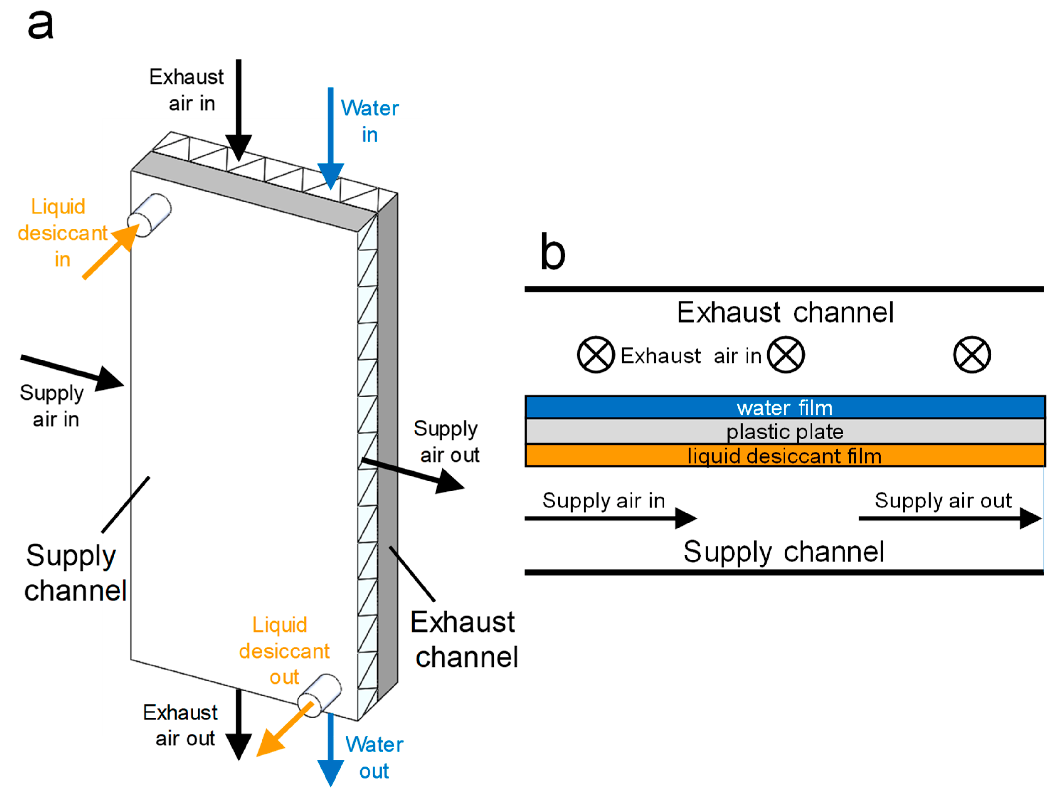
2.2. Heat and Mass Transfer Model

A schematic of a pair of supply and exhaust channels used to develop the heat and mass transfer model is shown in Figure 2. As shown in the figure, the supply air is flowing in the positive x direction, while the exhaust air and liquid desiccant are flowing in the negative y direction. The two-dimensional heat and mass transfer model of the dehumidifier is developed using a number of assumptions that are listed below [19]:

• The system is insulated; therefore, no heat transfer occurs between the device and the surroundings.
• The thickness of the channels is small relative to the channels’ length and width; therefore, the variations of temperature and humidity ratio normal to the flow are neglected, reducing the problem to be two-dimensional.
• The flow is laminar, fully developed, and steady.
• The mass flow rate is constant in each channel.
• The heat and mass transfer coefficients are constant.
• The heat and mass transfer analogy holds.

2.2.1. Governing Equations

Using the listed assumptions, the governing equations are formulated as follows.

Energy balance of the supply air:

$${\dot{m}}_{\mathrm{s}}{C}_{p,\mathrm{s}}\frac{\partial T_{\mathrm{s}}}{\partial x}=UW\left(T_{\mathrm{LD}}-T_{\mathrm{s}}\right)$$

(1)

where U is the overall heat transfer coefficient and is calculated using the following equation:

$$U={\left(\frac{1}{h_{\mathrm{s}}}+\frac{t_{\mathrm{membrane}}}{k_{\mathrm{membrane}}}\right)}^{-1}$$

(2)

where h is the convective heat transfer coefficient, t_membrane is the thickness of the membrane, and k_membrane is the thermal conductivity of the membrane.

Energy balance of the exhaust air:

$$-{\dot{m}}_{\mathrm{e}}{C}_{p,\mathrm{e}}\frac{\partial T_{\mathrm{e}}}{\partial y}=h_{\mathrm{e}}L\left(T_{\mathrm{wf}}-T_{\mathrm{e}}\right)$$

(3)

The specific heats of the supply and exhaust air are determined by the following equation:

$$C_p=C_{p,\mathrm{air}}+\omega C_{p,\mathrm{vapor}}$$

(4)

where ω is the humidity ratio, C_p,air (1007 J kg⁻¹ K⁻¹) is the specific heat of air, and C_p,vapor (1870 J kg⁻¹ K⁻¹) is the specific heat of water vapor at room temperature.

Moisture balance of the supply air:

$${\dot{m}}_{\mathrm{s}}\frac{\partial {\omega }_{\mathrm{s}}}{\partial x}=U_{\mathrm{m},\mathrm{s}}W\left({\omega }_{\mathrm{LD}}-{\omega }_{\mathrm{s}}\right)$$

(5)

where U_m,s is the overall mass transfer coefficient and is determined by the following formula:

$$U_{\mathrm{m},\mathrm{s}}={\left(\frac{1}{h_{\mathrm{m},\mathrm{s}}{\rho }_{\mathrm{air}}}+\frac{t_{\mathrm{membrane}}}{{\rho }_{\mathrm{air}}{D}_{\mathrm{membrane}}}\right)}^{-1}$$

(6)

ω_LD is the humidity ratio of air in equilibrium with the liquid desiccant film and is determined by:

$${\omega }_{\mathrm{LD}}=0.622\frac{{\mathrm{P}}_{\mathrm{LD}}}{P_{\mathrm{atm}}-P_{\mathrm{LD}}}$$

(7)

The properties of the liquid desiccant solution, including the saturated vapor pressure above the liquid desiccant film, P_LD, density, ρ_LD, thermal conductivity, k_LD, specific heat, C_p,LD, and enthalpy of dilution, h_dilution, are determined by correlations from Conde [20].

Moisture balance of the exhaust air:

$$-{\dot{m}}_{\mathrm{e}}\frac{\partial {\omega }_{\mathrm{e}}}{\partial y}=h_{\mathrm{m},\mathrm{e}}{\rho }_{air}L\left({\omega }_{\mathrm{wf}}-{\omega }_{\mathrm{e}}\right)$$

(8)

The saturated air humidity ratio, ω_wf, is determined by Equation (7), substituting P_LD with P_g, the pressure of the saturated vapor at the exhaust air temperature, which is calculated using the following equation [21,22]:

$$P_g=\left(611.21\right)e^{\left(\left(18.678-\frac{T_{\mathrm{e}}}{234.5}\right)\left(\frac{T_{\mathrm{e}}}{257.14+T_{\mathrm{e}}}\right)\right)}$$

(9)

Energy balance of the liquid desiccant film:

$$-{\dot{m}}_{\mathrm{LD}}{C}_{p,\mathrm{LD}}\frac{\partial T_{\mathrm{LD}}}{\partial y}+UL\left(T_{\mathrm{LD}}-T_{\mathrm{s}}\right)+U_{ms}L\left({\omega }_{\mathrm{LD}}-{\omega }_{\mathrm{s}}\right)\left(h_{\mathrm{dilution}}+h_{fg}\right)+U_{\mathrm{plate}}L\left(T_{\mathrm{LD}}-T_{\mathrm{wf}}\right)=0$$

(10)

h_fg is calculated by [23]:

$$h_{fg}={10}^3\left(2501-2.369T_{\mathrm{wf}}\right)$$

(11)

The overall heat transfer coefficient of the plastic plate, U_plate, is calculated as follows:

$$U_{\mathrm{plate}}={\left(\frac{t_{\mathrm{wick}}}{k_{\mathrm{LD}}}+\frac{t_{\mathrm{plate}}}{k_{\mathrm{plate}}}+\frac{t_{\mathrm{wick}}}{k_{\mathrm{wf}}}\right)}^{-1}$$

(12)

Energy balance of the water film:

$$h_{e}L\left(T_{wf}-T_e\right)+h_{me}{\rho }_{air}L\left({\omega }_{wf}-{\omega }_e\right)h_{fg}-U_{\mathrm{plate}}L\left(T_{LD}-T_{wf}\right)=0$$

(13)

Equations (1), (3), (5), (8), (10), and (13) are the governing heat and mass transfer equations of the internally-cooled liquid desiccant dehumidifier. The governing equations were solved using Newton’s method and convergence was assumed to be obtained when the relative residuals of the governing equations were less than 10⁻⁴.

2.2.2. Boundary Conditions

The governing equations are completed by the following boundary conditions. The supply air temperature and humidity ratio are specified at x = 0, Equations (14) and (15). At y = W, the top boundary of the supply channel, the liquid desiccant temperature is specified, Equation (16). The exhaust air temperature and humidity ratio are specified at the inlet of the exhaust channel, at y = W, Equations (17) and (18).

$$T_{\mathrm{s}}\left(0, y\right)=T_{\mathrm{s},\mathrm{in}}$$

(14)

$${\omega }_{\mathrm{s}}\left(0, y\right)={\omega }_{\mathrm{s},\mathrm{in}}$$

(15)

$$T_{\mathrm{LD}}\left(x, W\right)=T_{\mathrm{LD},\mathrm{in}}$$

(16)

$$T_{\mathrm{e}}\left(x,W\right)=T_{\mathrm{e},\mathrm{in}}$$

(17)

$${\omega }_{\mathrm{e}}\left(x, W\right)={\omega }_{\mathrm{e},\mathrm{in}}$$

(18)

2.2.3. Heat and Mass Transfer Coefficients

Using the following formula, the convective heat transfer coefficient is determined:

$$h=\frac{Nu{k}_{\mathrm{air}}}{d_{\mathrm{h}}}$$

(19)

The Nusselt number, Nu, for parallel plates is assumed to be equal to the average of the constant wall temperature boundary condition (7.541) and constant heat flux (8.235) boundary condition values [24], since the boundary condition at the channel walls is neither constant temperature nor constant heat flux.

The mass transfer coefficient in the supply and exhaust channels is calculated as follows:

$$h_m=\frac{Sh{D}_{\mathrm{va}}}{d_{\mathrm{h}}}$$

(20)

where Sh is the Sherwood number, and D_va is the binary diffusion coefficient of water vapor in air. Given that the heat and mass transfer analogy holds, the Sherwood number is considered equal to the Nusselt number.

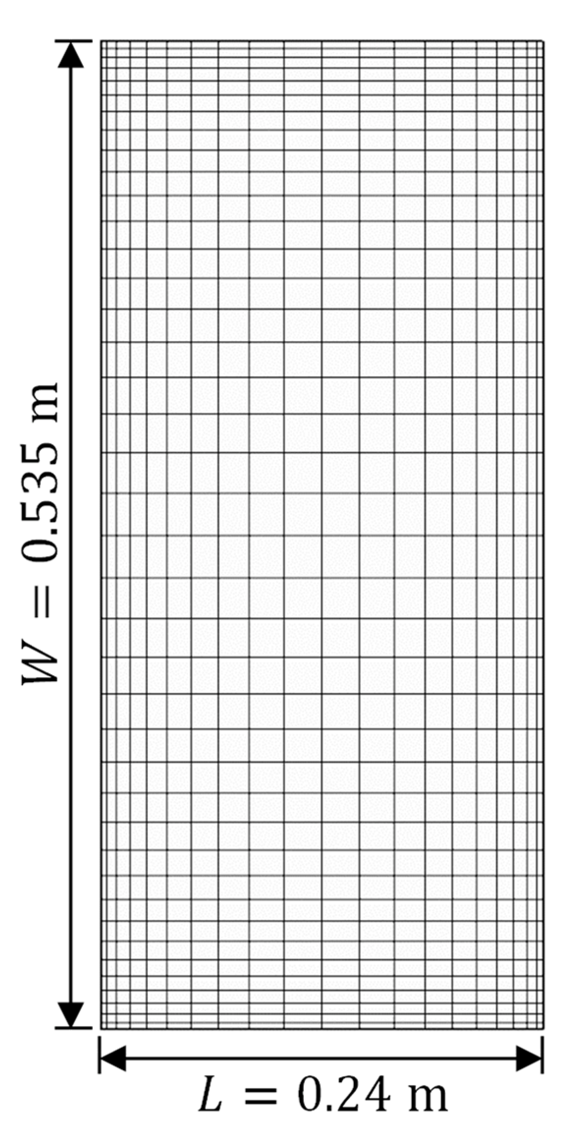
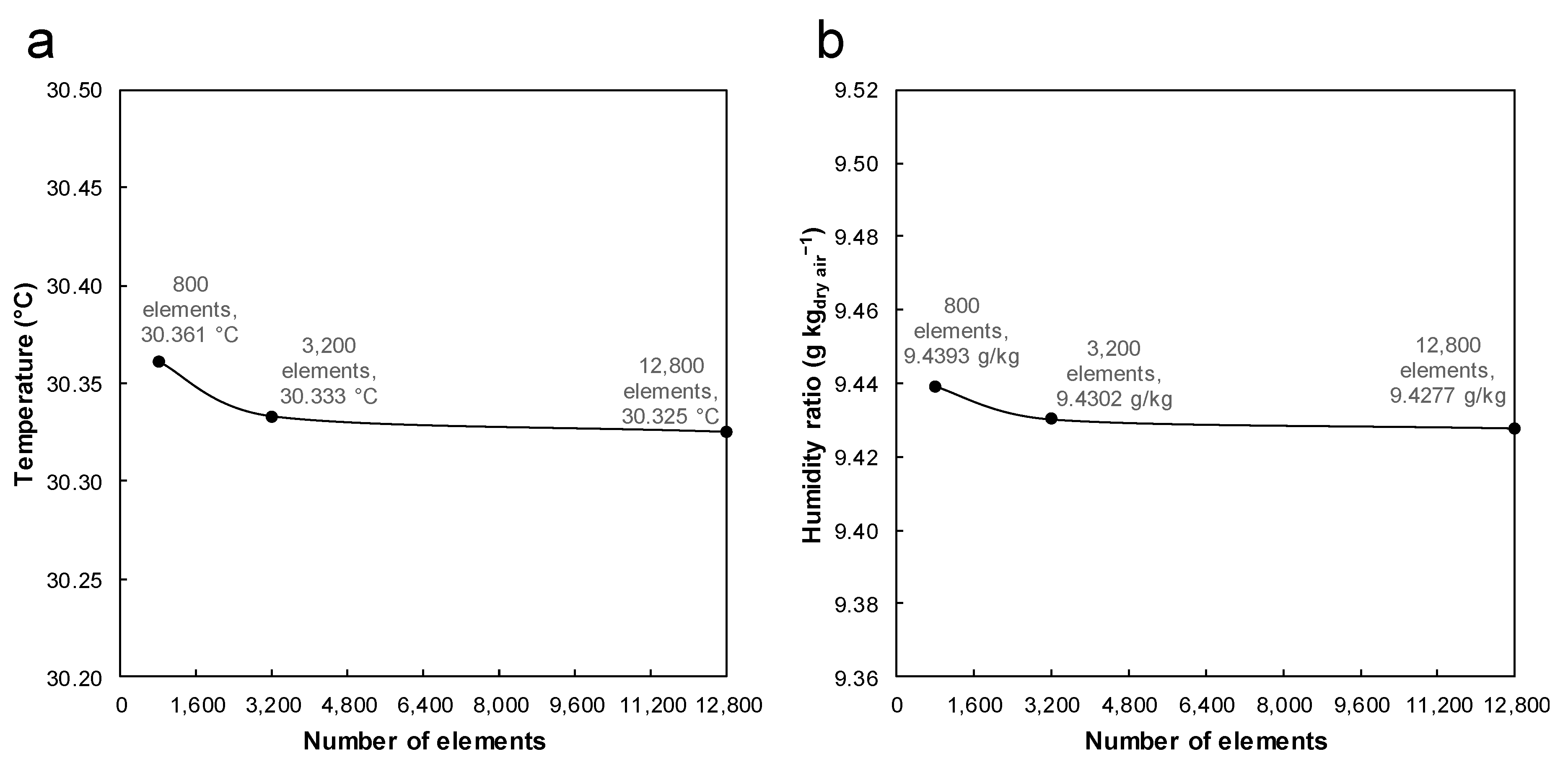
2.2.4. Computational Grid

The system of equations governing the heat and mass transfer in the internally-cooled liquid desiccant dehumidifier was discretized and solved using the finite element method. The computational domain, Figure 3, was discretized using a structured mesh with quadrilateral elements. The length and width of the domain were divided into 20 and 40 elements, respectively. The elements along the length and width were distributed using a symmetric arithmetic sequence with an element ratio of 6. Two additional grids were created by doubling the number of divisions along the length and width, twice, which changed the obtained supply air outlet conditions by less than 0.1%. Figure 4 shows the obtained supply air outlet temperature and humidity ratio using the three computational grids. Therefore, it was concluded that the results obtained by the mesh shown in Figure 3 are grid-independent.

2.3. Regression Models

Response surface methodology was used to analyze and model the influence of several operational and geometrical factors on the supply air outlet humidity ratio, ω_s,out, and supply air outlet temperature, T_s,out, of internally-cooled liquid desiccant dehumidifiers. To fit quadratic response models in 12 factors, the central composite design was used.

Table 2. The level of the factors in the CCD.

No.	Factor	Description	Unit	Levels
1	Ts,in	Supply air inlet temperature	°C	20	26.5	33	39.5	46
2	ωs,in	Supply air inlet humidity ratio	kg/kg	0.011	0.0145	0.018	0.0215	0.025
3	Te,in	Exhaust air inlet temperature	°C	24	29.5	35	40.5	46
4	ωe,in	Exhaust air inlet humidity ratio	kg/kg	0.011	0.0145	0.018	0.0215	0.025
5	TLD,in	Liquid desiccant inlet temperature	°C	24	29.5	35	40.5	46
6	CLD	Liquid desiccant concentration	kg/kg	0.32	0.375	0.43	0.485	0.54
7	vLD	Liquid desiccant flow rate per channel	mL/min	7	9.75	12.5	15.25	18
8	${\dot{m}}_{\mathrm{s}}$	Supply air mass flow rate per channel	kg/s	0.0024	0.0033	0.0042	0.0051	0.006
9	r	Ratio of exhaust to supply mass flow rate	-	0	0.25	0.5	0.75	1
10	t	Thickness of the channels	mm	2	3	4	5	6
11	L	Channel length	m	0.15	0.2625	0.375	0.4875	0.6
12	W	Channel width	m	0.15	0.2625	0.375	0.4875	0.6

shows the 12 considered factors and their levels, which include supply inlet temperature, T_s,in, supply inlet humidity ratio, ω_s,in, exhaust inlet temperature, T_e,in, exhaust inlet humidity ratio, ω_e,in, liquid desiccant inlet temperature, T_LD,in, liquid desiccant concentration, C_LD, liquid desiccant flow rate per channel, v_LD, supply air mass flow rate per channel, ${\dot{m}}_{\mathrm{s}}$, ratio of exhaust to supply air mass flow rate, r (${\dot{m}}_{\mathrm{e}}/{\dot{m}}_{\mathrm{s}}$), thickness of the channels, t, channel length, L, and channel width, W. The range of the considered factors, for example, supply temperature and humidity ratio, is selected so that a wide range of possible weather conditions is covered in the developed regression models. The distance between the axial and center points (α value) is 2. The designed experimental runs were performed using the two-dimensional numerical model presented in Section 2.2. The central composite design matrix, which consists of 546 runs, and the calculated responses using the numerical heat and mass transfer model are provided in Table S1 (Supplementary material).

3. Results and Discussion

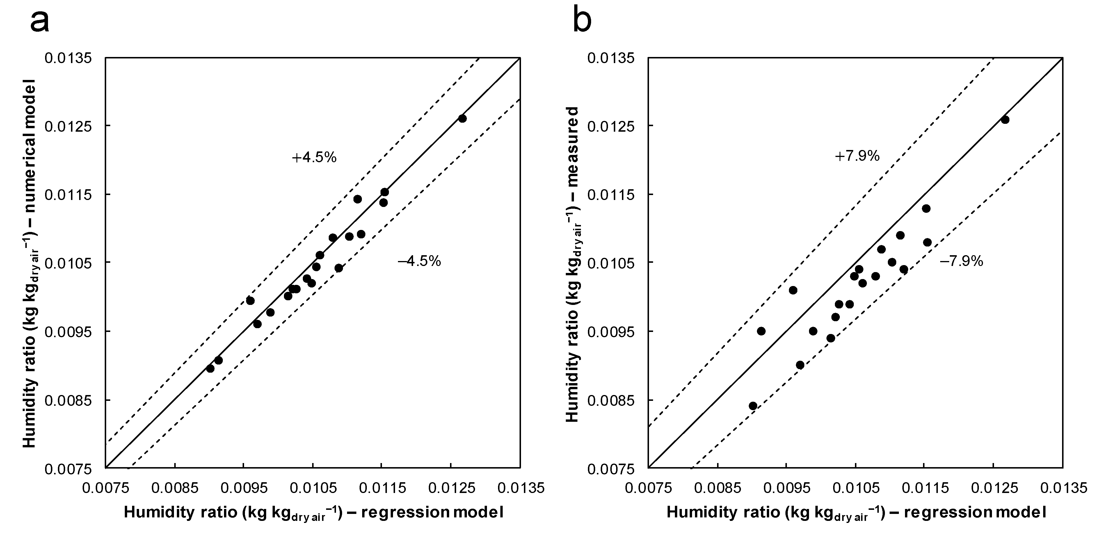
3.1. Validation of the Heat and Mass Transfer Model

To validate the numerical heat and mass transfer model, the predicted supply air outlet humidity ratio of the experimental test conditions listed in Table A1 is compared to the measured values [7]. Figure 5 shows a comparison between the measured and numerical model predictions of the supply air outlet humidity ratio. The data labels in the figure represent the test numbers from Table A1. As shown in the figure, the model predictions match the measured values within 6.7%. The average difference between the predictions and measured values is about 3.7%. As shown in the figure, at approximately 80% of the tests, the numerical model overpredicted the experimental measurements. The maximum difference is at test 6 (6.7%), while the minimum difference is at test 8 (0.1%).

3.2. Regression Models

3.2.1. Supply Air Outlet Humidity Ratio

A quadratic model with the supply air humidity ratio, ω_s,out, as the response is fitted to the central composite design matrix (Table S1, Supplementary material). The analysis of variance (ANOVA) for the reduced model using backward elimination with a p-value of 0.05 is summarized in

Table A2. ANOVA for the supply air outlet humidity ratio regression model.

Source	Coded Coefficient × 10−5	DF	Adj SS × 10−10	Adj MS × 10−5	F-Value	p-Value
Model		60	53,742,256	895,704.3	3677.432	0.000
Linear		12
Ts,in	23.58	1	289,105.9	289,105.9	1186.96	0.000
ωs,in	193.56	1	19,481,938	19,481,938	79,985.66	0.000
Te,in	10.42	1	56,475.98	56,475.98	231.87	0.000
ωe,in	15.88	1	131,123.1	131,123.1	538.34	0.000
TLD,in	7.69	1	30,730.78	30,730.78	126.17	0.000
CLD	−124.66	1	8,080,975	8,080,975	33,177.5	0.000
vLD	−0.38	1	76.78	76.78	0.32	0.575
${\dot{m}}_{\mathrm{s}}$	85.83	1	3,830,366	3,830,366	15,726.07	0.000
r	−23.23	1	280,592.4	280,592.4	1152.01	0.000
t	80.84	1	3,398,203	3,398,203	13,951.77	0.000
L	−122.5	1	7,803,524	7,803,524	32,038.4	0.000
W	−121.81	1	7,715,903	7,715,903	31,678.66	0.000
Square		6
CLD2	13.83	1	7010.6	7010.6	28.78	0.000
${\dot{m}}_{\mathrm{s}}^2$	−17.23	1	10,872.96	10,872.96	44.64	0.000
r2	29.96	1	32,870.27	32,870.27	134.95	0.000
t2	−15.6	1	8915.74	8915.74	36.6	0.000
L2	12.02	1	5288.41	5288.41	21.71	0.000
W2	11.85	1	5143.08	5143.08	21.12	0.000
2-Way Interaction		42
Ts,inωs,in	1.49	1	1131.63	1131.63	4.65	0.032
Ts,inCLD	−8.07	1	33,330.72	33,330.72	136.84	0.000
$T_{\mathrm{s},\mathrm{in}}{\dot{m}}_{\mathrm{s}}$	−2.31	1	2743.74	2743.74	11.26	0.001
Ts,inr	−3.51	1	6309.72	6309.72	25.91	0.000
Ts,int	−4.34	1	9655.98	9655.98	39.64	0.000
Ts,inL	4.05	1	8408.94	8408.94	34.52	0.000
Ts,inW	3.98	1	8099.78	8099.78	33.25	0.000
ωs,inCLD	−9.31	1	44,363.64	44,363.64	182.14	0.000
${\omega }_{\mathrm{s},\mathrm{in}}{\dot{m}}_{\mathrm{s}}$	21.03	1	226,454.4	226,454.4	929.74	0.000
ωs,inr	−4.98	1	12,704.38	12,704.38	52.16	0.000
ωs,int	19.39	1	192,575.3	192,575.3	790.64	0.000
ωs,inL	−29.45	1	443,914	443,914	1822.55	0.000
ωs,inW	−29.28	1	438,928.3	438,928.3	1802.08	0.000
Te,inCLD	−3.66	1	6846.26	6846.26	28.11	0.000
Te,int	−1.37	1	955.12	955.12	3.92	0.048
Te,inL	2.07	1	2192.54	2192.54	9	0.003
Te,inW	2.07	1	2198.43	2198.43	9.03	0.003
ωe,inCLD	−5.59	1	15,970.64	15,970.64	65.57	0.000
${\omega }_{\mathrm{e},\mathrm{in}}{\dot{m}}_{\mathrm{s}}$	−1.93	1	1909	1909	7.84	0.005
ωe,inr	1.7	1	1475.81	1475.81	6.06	0.014
ωe,int	−1.99	1	2032.19	2032.19	8.34	0.004
ωe,inL	3.05	1	4774.97	4774.97	19.6	0.000
ωe,inW	3.05	1	4753.86	4753.86	19.52	0.000
TLD,inCLD	−2.79	1	3976.76	3976.76	16.33	0.000
TLD,invLD	2.4	1	2939.05	2939.05	12.07	0.001
$T_{\mathrm{LD},\mathrm{in}}{\dot{m}}_{\mathrm{s}}$	−1.85	1	1758.02	1758.02	7.22	0.007
TLD,inr	−1.39	1	985.79	985.79	4.05	0.045
$C_{\mathrm{LD}}{\dot{m}}_{\mathrm{s}}$	16.93	1	146,756	146,756	602.53	0.000
CLDr	4.96	1	12,587.89	12,587.89	51.68	0.000
CLDt	16.79	1	144,343	144,343	592.62	0.000
CLDL	−23.91	1	292,820	292,820	1202.21	0.000
CLDW	−23.73	1	288,329	288,329	1183.77	0.000
${\dot{m}}_{\mathrm{s}}$r	5.34	1	14,616.65	14,616.65	60.01	0.000
${\dot{m}}_{\mathrm{s}}$t	−3.34	1	5724.1	5724.1	23.5	0.000
${\dot{m}}_{\mathrm{s}}$L	5.61	1	16,123.14	16,123.14	66.2	0.000
${\dot{m}}_{\mathrm{s}}$W	5.55	1	15,755.57	15,755.57	64.69	0.000
rt	5.27	1	14,223.52	14,223.52	58.4	0.000
rL	−8.22	1	34,587.46	34,587.46	142	0.000
rW	−8.2	1	34,408.51	34,408.51	141.27	0.000
tL	4.98	1	12,697.8	12,697.8	52.13	0.000
tW	5.07	1	13,167.6	13,167.6	54.06	0.000
LW	−8.17	1	34,146.68	34,146.68	140.19	0.000
Error		485	118,130.4	243.5679
Total		545	53,860,387

. DF, Adj SS, and Adj MS stand for degrees of freedom, adjusted sum of squares, and adjusted mean sum of squares, respectively. The regression model terms are assessed according to a significance level of 0.05, that is, terms that have a p-value of less than 0.05 are considered significant. The statistical analysis showed that among the main factors, v_LD has no significant effect on the outlet humidity ratio since its p-value is more than 0.05, which is in line with experimental results [7]. Half of the square terms are significant, C_LD², ${{\dot{m}}_{\mathrm{s}}}^2$, r², t², L², and W², while only 42 of the 66 interaction terms have p-value of less than 0.05.

The coded coefficients of the factors are shown in Table A2. Given that the coded coefficients are dimensionless, the relative effect of the factors can be determined by comparing the magnitude and sign of their coded coefficients. Therefore, as shown in the table, the supply air inlet humidity ratio has the most significant effect on the outlet air humidity ratio. The lower the inlet air humidity ratio, the lower the outlet air humidity ratio. The second significant factor is the liquid desiccant concentration, C_LD, which is inversely proportional to the outlet air humidity ratio; the higher the liquid desiccant concentration, the lower the outlet air humidity ratio and the more efficient the dehumidifying process. The channels’ length and width have almost equal effect on the outlet air humidity ratio. Then there is the mass flow rate of the supply air, with its effect being less than half of the inlet air humidity ratio. From the main significant factors, the temperature of the liquid desiccant has the least effect on the outlet air humidity ratio. As shown in the table, some square terms, r², and interaction terms, for example, r², ω_s,inL, and ω_s,inW, are more significant than some of the main factors.

After removing the terms that are not significant using backward elimination, a regression model with the supply air outlet humidity ratio as the response with a reduced number of terms is obtained. The coefficient of determination (R²) of the regression model is 0.9978; therefore, about 99.78% of the variability in the supply air outlet humidity ratio is explained by the model. It should be noted that the main factor, $v_{\mathrm{L}\mathrm{D}}$, which has no significant effect on the outlet air humidity ratio, is included in the model to keep the model hierarchical since its interaction with T_LD,in is significant. The obtained regression model is:

$$\begin{array}{cc}\hfill {\omega }_{\mathrm{s},\mathrm{out}}& ={10}^{-5}(332.62527+13.45256 T_{\mathrm{s},\mathrm{in}}+82508.26867 {\omega }_{\mathrm{s},\mathrm{in}}+5.57611 T_{\mathrm{e},\mathrm{in}}+15083.53088 {\omega }_{\mathrm{e},\mathrm{in}}\hfill \\ & +5.45609 T_{\mathrm{LD},\mathrm{in}}-3266.92378 C_{\mathrm{LD}}-5.68396 v_{\mathrm{LD}}+5633.09943 {\dot{m}}_s-518.28366 r\hfill \\ & -12.82095 t+745.78794 L+743.98583 W+ 4573.24261 C_{\mathrm{LD}}^2-21269680.36043 {\dot{m}}_s^2\hfill \\ & +479.28494 r^2-15.60094 t^2+949.35774 L^2+936.22194 W^2+65.34856 T_{\mathrm{s},\mathrm{in}}{\omega }_{\mathrm{s},\mathrm{in}}\hfill \\ & -22.56895 T_{\mathrm{s},\mathrm{in}}{C}_{\mathrm{LD}}-395.71314 T_{\mathrm{s},\mathrm{in}}{\dot{m}}_s-2.16031 T_{\mathrm{s},\mathrm{in}}r-0.66811 T_{\mathrm{s},\mathrm{in}}t+5.54204 T_{\mathrm{s},\mathrm{in}}L\hfill \\ & +5.43921 T_{\mathrm{s},\mathrm{in}}W-48355.7224 {\omega }_{\mathrm{s},\mathrm{in}}{C}_{\mathrm{LD}}+6676438.49206 {\omega }_{\mathrm{s},\mathrm{in}}{\dot{m}}_s-5692.90179 {\omega }_{\mathrm{s},\mathrm{in}}r\hfill \\ & +5541.11607 {\omega }_{\mathrm{s},\mathrm{in}}t-74781.44841 {\omega }_{\mathrm{s},\mathrm{in}}L-74360.31746 {\omega }_{\mathrm{s},\mathrm{in}}W-12.08833 T_{\mathrm{e},\mathrm{in}}{C}_{\mathrm{LD}}\hfill \\ & -0.24833 T_{\mathrm{e},\mathrm{in}}t+3.34444 T_{\mathrm{e},\mathrm{in}}L+3.34893 T_{\mathrm{e},\mathrm{in}}W-29013.18994 {\omega }_{\mathrm{e},\mathrm{in}}{C}_{\mathrm{LD}}\hfill \\ & -612996.03175 {\omega }_{\mathrm{e},\mathrm{in}}{\dot{m}}_s+1940.3125 {\omega }_{\mathrm{e},\mathrm{in}}r-569.21875 {\omega }_{\mathrm{e},\mathrm{in}}t+7755.85317 {\omega }_{\mathrm{e},\mathrm{in}}L\hfill \\ & +7738.69048 {\omega }_{\mathrm{e},\mathrm{in}}W-9.21307 T_{\mathrm{LD},\mathrm{in}}{C}_{\mathrm{LD}}+0.15841 T_{\mathrm{LD},\mathrm{in}}{v}_{\mathrm{LD}}-374.34501 T_{\mathrm{LD},\mathrm{in}}{\dot{m}}_s\hfill \\ & -1.00915 T_{\mathrm{LD},\mathrm{in}}r+342024.93687 C_{\mathrm{LD}}{\dot{m}}_s+360.6108 C_{\mathrm{LD}}r+305.28125 C_{\mathrm{LD}}t\hfill \\ & -3865.00631 C_{\mathrm{LD}}L-3835.25253 C_{\mathrm{LD}}W+23746.875 {\dot{m}}_{s}r-3715.14757 {\dot{m}}_{s}t\hfill \\ & +55423.61111 {\dot{m}}_{s}L+54788.19444 {\dot{m}}_{s}W+21.08281 rt-292.23472 rL-291.47778 rW\hfill \\ & +44.26667 tL+45.07812 tW-645.25926 LW)\hfill \end{array}$$

(21)

3.2.2. Supply Air Outlet Temperature

The ANOVA for the reduced model using backward elimination with a p-value of 0.05 with the supply air outlet temperature, T_s,out, as the response is shown in

Table A3. ANOVA for the supply air outlet temperature regression model.

Source	Coded Coefficient	DF	Adj SS	Adj MS	F-Value	p-Value
Model		59	7503.37	127.18	1747.11	0.000
Linear		12
Ts,in	3.2351	1	5442.19	5442.19	74,763.64	0.000
ωs,in	0.9002	1	421.37	421.37	5788.68	0.000
Te,in	0.3522	1	64.52	64.52	886.33	0.000
ωe,in	0.5377	1	150.33	150.33	2065.14	0.000
TLD,in	0.2616	1	35.58	35.58	488.82	0.000
CLD	0.7573	1	298.19	298.19	4096.41	0.000
vLD	−0.0142	1	0.1	0.1	1.44	0.231
${\dot{m}}_{\mathrm{s}}$	−0.0772	1	3.1	3.1	42.54	0.000
r	−0.7296	1	276.84	276.84	3803.12	0.000
t	−0.2364	1	29.07	29.07	399.38	0.000
L	0.1461	1	11.1	11.1	152.45	0.000
W	0.1378	1	9.88	9.88	135.67	0.000
Square		7
ωs,in2	−0.1034	1	0.39	0.39	5.3	0.022
ωe,in2	−0.0987	1	0.35	0.35	4.82	0.029
CLD2	−0.1894	1	1.29	1.29	17.77	0.000
${\dot{m}}_{\mathrm{s}}^2$	−0.1068	1	0.41	0.41	5.65	0.018
r2	0.7185	1	18.61	18.61	255.61	0.000
L2	−0.1428	1	0.73	0.73	10.1	0.002
W2	−0.1404	1	0.71	0.71	9.76	0.002
2-Way Interaction		40
$T_{\mathrm{s},\mathrm{in}}{\dot{m}}_{\mathrm{s}}$	0.4097	1	85.95	85.95	1180.82	0.000
Ts,inr	−0.0738	1	2.79	2.79	38.33	0.000
Ts,int	0.4953	1	125.6	125.6	1725.4	0.000
Ts,inL	−0.5692	1	165.87	165.87	2278.63	0.000
Ts,inW	−0.5647	1	163.28	163.28	2243.11	0.000
ωs,inωe,in	−0.0254	1	0.33	0.33	4.53	0.034
ωs,inCLD	0.0427	1	0.94	0.94	12.85	0.000
${\omega }_{\mathrm{s},\mathrm{in}}{\dot{m}}_{\mathrm{s}}$	−0.0854	1	3.73	3.73	51.27	0.000
ωs,inr	−0.0771	1	3.04	3.04	41.77	0.000
ωs,int	−0.1566	1	12.55	12.55	172.38	0.000
ωs,inL	0.1477	1	11.17	11.17	153.44	0.000
ωs,inW	0.1453	1	10.8	10.8	148.42	0.000
$T_{\mathrm{e},\mathrm{in}}{\dot{m}}_{\mathrm{s}}$	−0.0418	1	0.89	0.89	12.29	0.000
Te,inr	0.0503	1	1.29	1.29	17.79	0.000
Te,int	−0.0579	1	1.72	1.72	23.58	0.000
Te,inL	0.0662	1	2.24	2.24	30.82	0.000
Te,inW	0.0662	1	2.24	2.24	30.82	0.000
${\omega }_{\mathrm{e},\mathrm{in}}{\dot{m}}_{\mathrm{s}}$	−0.0616	1	1.95	1.95	26.72	0.000
ωe,inr	0.0835	1	3.57	3.57	49.07	0.000
ωe,int	−0.0855	1	3.74	3.74	51.44	0.000
ωe,inL	0.0979	1	4.9	4.9	67.38	0.000
ωe,inW	0.0977	1	4.89	4.89	67.13	0.000
TLD,invLD	0.0344	1	0.61	0.61	8.33	0.004
$T_{\mathrm{LD},\mathrm{in}}{\dot{m}}_{\mathrm{s}}$	−0.0607	1	1.89	1.89	25.95	0.000
TLD,inr	−0.0404	1	0.84	0.84	11.48	0.001
$C_{\mathrm{LD}}{\dot{m}}_{\mathrm{s}}$	−0.0557	1	1.59	1.59	21.81	0.000
CLDr	−0.108	1	5.97	5.97	82.08	0.000
CLDt	−0.1272	1	8.28	8.28	113.74	0.000
CLDL	0.1076	1	5.92	5.92	81.37	0.000
CLDW	0.1042	1	5.56	5.56	76.33	0.000
${\dot{m}}_{\mathrm{s}}$r	0.1533	1	12.04	12.04	165.37	0.000
${\dot{m}}_{\mathrm{s}}$t	−0.0426	1	0.93	0.93	12.78	0.000
${\dot{m}}_{\mathrm{s}}$L	0.0607	1	1.89	1.89	25.91	0.000
${\dot{m}}_{\mathrm{s}}$W	0.0612	1	1.92	1.92	26.32	0.000
rt	0.1762	1	15.89	15.89	218.28	0.000
rL	−0.2396	1	29.38	29.38	403.67	0.000
rW	−0.239	1	29.24	29.24	401.75	0.000
tL	0.0512	1	1.34	1.34	18.47	0.000
tW	0.0493	1	1.25	1.25	17.12	0.000
LW	−0.0774	1	3.07	3.07	42.16	0.000
Error		486	35.38	0.07
Total		545	7538.75

. As shown in the table, the main factor, v_LD, has no significant effect on the supply air outlet temperature. From the square terms, only seven have significant effect: ω_s,in², ω_e,in², C_LD², ${\dot{m}}_{\mathrm{s}}^2$, r², L², and W². From the interaction terms, only 40 out of the 66 have significant effect on the outlet air temperature. It should be noted that even though the effect of the main factor v_LD was not significant, its interaction with T_LD,in is significant, as shown in the table. From the coded coefficients, it can be seen that the supply air inlet temperature is the most significant factor affecting the supply air outlet temperature followed by supply air inlet humidity ratio, the liquid desiccant concentration, and the exhaust to supply mass flow rate ratio.

After removing the terms that are not significant using backward elimination, a reduced regression model for the supply air outlet temperature is obtained. The R² of the model is 0.9953 which indicates that up to 99.53% of the total variance can be explained by this model:

$$\begin{array}{cc}\hfill T_{\mathrm{s},\mathrm{out}}& =-17.78584+0.50295 T_{\mathrm{s},\mathrm{in}}+560.68845 {\omega }_{\mathrm{s},\mathrm{in}}+0.0431 T_{\mathrm{e},\mathrm{in}}+426.78387 {\omega }_{\mathrm{e},\mathrm{in}}+0.08534 T_{\mathrm{LD},\mathrm{in}}\hfill \\ & +68.68971 C_{\mathrm{LD}}-0.08481 v_{\mathrm{LD}}+156.5784 {\dot{m}}_s-9.22115 r-0.63201 t+15.21398 L\hfill \\ & +15.19101 W-8441.6389 {\omega }_{\mathrm{s},\mathrm{in}}^2-8053.8838 {\omega }_{\mathrm{e},\mathrm{in}}^2-62.6149 C_{\mathrm{LD}}^2-131833.42782 {\dot{m}}_s^2\hfill \\ & +11.49544 r^2-11.28178 L^2-11.09413 W^2+70.0394 T_{\mathrm{s},\mathrm{in}}{\dot{m}}_s-0.04543 T_{\mathrm{s},\mathrm{in}}r\hfill \\ & +0.0762 T_{\mathrm{s},\mathrm{in}}t-0.77835 T_{\mathrm{s},\mathrm{in}}L-0.77226 T_{\mathrm{s},\mathrm{in}}W-2072.06633 {\omega }_{\mathrm{s},\mathrm{in}}{\omega }_{\mathrm{e},\mathrm{in}}\hfill \\ & +222.03734 {\omega }_{\mathrm{s},\mathrm{in}}{C}_{\mathrm{LD}}-27103.1746 {\omega }_{\mathrm{s},\mathrm{in}}{\dot{m}}_s-88.07143 {\omega }_{\mathrm{s},\mathrm{in}}r-44.72879 {\omega }_{\mathrm{s},\mathrm{in}}t\hfill \\ & +375.10913 {\omega }_{\mathrm{s},\mathrm{in}}L+368.91865 {\omega }_{\mathrm{s},\mathrm{in}}W-8.4446 T_{\mathrm{e},\mathrm{in}}{\dot{m}}_s+0.03657 T_{\mathrm{e},\mathrm{in}}r-0.01053 T_{\mathrm{e},\mathrm{in}}t\hfill \\ & +0.10698 T_{\mathrm{e},\mathrm{in}}L+0.10698 T_{\mathrm{e},\mathrm{in}}W-19567.2123 {\omega }_{\mathrm{e},\mathrm{in}}{\dot{m}}_s+95.45982 {\omega }_{\mathrm{e},\mathrm{in}}r\hfill \\ & -24.43304 {\omega }_{\mathrm{e},\mathrm{in}}t+248.57143 {\omega }_{\mathrm{e},\mathrm{in}}L+248.11508 {\omega }_{\mathrm{e},\mathrm{in}}W+0.00228 T_{\mathrm{LD},\mathrm{in}}{v}_{\mathrm{LD}}\hfill \\ & -12.27036 T_{\mathrm{LD},\mathrm{in}}{\dot{m}}_s-0.02938 T_{\mathrm{LD},\mathrm{in}}r-1124.92109 C_{\mathrm{LD}}{\dot{m}}_s-7.85653 C_{\mathrm{LD}}r\hfill \\ & -2.31207 C_{\mathrm{LD}}t+17.38258 C_{\mathrm{LD}}L+16.83586 C_{\mathrm{LD}}W+681.47569 {\dot{m}}_{s}r-47.36979 {\dot{m}}_{s}t\hfill \\ & +599.38272 {\dot{m}}_{s}L+604.16667 {\dot{m}}_{s}W+0.70466 rt-8.51778 rL-8.4975 rW+0.45545 tL\hfill \\ & +0.43851 tW-6.11698 LW\hfill \end{array}$$

(22)

3.3. Model–Experiments Comparison

Figure 6a compares the estimated supply air outlet humidity ratio by the regression and numerical models for the 20 test conditions in Table A1. As shown in the figure, the maximum difference between the estimations of the two models is about 4.5%, the minimum difference is 0%, and the average difference is about 1.5%.

The regression model’s estimates of the supply air outlet humidity ratio match the measured values within 7.9% (Figure 6b), with a minimum difference of 0.5% and an average difference of about 4.4%. Similar to the numerical model performance, for the majority of the tests, the regression model predicted higher outlet humidity ratios compared to the measured values.

3.4. Performance Assessment of the Dehumidification Process

The main purpose of the dehumidifier is to reduce the humidity ratio of the supply air. Therefore, to better understand the effect of the considered input factors, the plots of the 12 main effects of the factors on the supply air outlet humidity ratio are shown in Figure 7. In each plot, one factor is varied thorough its levels while the other factors are kept at their respective average levels.

The factors can be divided into four groups. The first group includes the supply and exhaust air inlet conditions, T_s,in, ω_s,in, T_e,in, and ω_e,in. The second group includes the liquid desiccant conditions, T_LD,in, C_LD, and v_LD. The third group includes the operational parameters, the supply air mass flow rate and the exhaust to supply air mass flow rate ratio, ${\dot{m}}_{\mathrm{s}}$ and r. The fourth group includes the geometrical properties of the dehumidifier, t, L, and W.

From the factors in the first group, varying the exhaust air inlet temperature and humidity ratio through their levels has little effect on the dehumidification process, with the dehumidification being more effective at their respective low levels. The reason for this behavior is that at the lower levels of exhaust air temperature and humidity ratio, the evaporative cooling potential in the exhaust channel increases, which leads to an improvement in the obtained dehumidification. Increasing the supply air inlet temperature has a negative effect on the dehumidification of the supply air. Increasing the supply air inlet temperature leads to an increase in the temperature of the liquid desiccant solution which lowers its dehumidification potential. Even though the effect of the supply air inlet temperature is higher than the previous factors, it is still not quite significant. In contrast to the previous factors, the effect of the supply air inlet humidity ratio is quite significant. Increasing the supply air inlet humidity ratio leads to an increase in supply air outlet humidity ratio; however, the amount of moisture removed increases as well.

From the factors in the second group, increasing the liquid desiccant inlet temperature has no significant effect on the dehumidification process; this is mainly due to the cooling effect from the exhaust channel. However, increasing the liquid desiccant concentration through its levels significantly affects the dehumidification of the supply air, with the most dehumidification being reached at the highest concentration level. The supply air outlet humidity ratio remains almost unchanged when changing the liquid desiccant flow rate through its levels.

From the third group, increasing the supply air mass flow rate leads to higher supply air outlet humidity ratio; that is, less dehumidification. Increasing the ratio of the exhaust to supply air mass flow rate improves the dehumidification; however, it reaches an optimum level between 50% and 75%, beyond which, increasing the mass flow rate ratio has a negative effect on the dehumidification process. This is in agreement with experimental results by Park et al. (2019); however, this could be due to the fact that models developed using a central composite design have poor predictability at the factor extremes relative to the central region of the factors.

From the last group, the smaller the channel thickness, the lower the supply air outlet humidity ratio. The effects of the length and width of the channels are relatively significant, with their effect being almost identical; lower supply air outlet humidity ratio is obtained for longer channels.

From the considered factors, the supply air inlet humidity ratio has the most significant effect on the dehumidification process. However, it should be noted that this factor cannot be controlled as it depends on the weather condition or the return air (if circulation is considered). Therefore, from the controllable factors, the most significant factor that affects the dehumidification process is the liquid desiccant concentration, followed by the dimensions of the channels.

3.5. Example of Using the Regression Models

The developed regression models, Equations (21) and (22), can be used to estimate the supply air outlet conditions of an internally-cooled liquid desiccant dehumidifier. Here, an example of using these equations is presented. The units and the range of input factors are listed in Table 2. Similar to the experiments, the liquid desiccant is assumed to be lithium chloride. The measured ambient air temperature and relative humidity during a humid day in Qatar are used as the supply air conditions. The exhaust air inlet conditions are considered equal to the supply air inlet conditions. The supply air mass flow rate is set to 0.15 kg/s and the ratio of the exhaust to supply air mass flow rate is set to 0.65. The temperature and concentration of the liquid desiccant are set to 35 °C and 0.5, respectively. The dimensions of the dehumidifier, including number of channels (36), length (0.24 m) of channels, and width (0.535) of channels, are set as the experiments.

It is assumed that the dehumidifier is used in combination with a counter flow dew point evaporative cooling system. For predicting the outlet air conditions of the evaporative cooling system, the regression models developed by Pakari and Ghani [25] are used. The specifications of the cooling system are as follows. Number of channels, 80, channel length, 0.55 m, channel width, 0.35 m, channel thickness, 2.2 mm, and extraction ratio, 40%.

Figure 8a,b show the ambient air temperature and relative humidity during a humid day (16 June 2017) in Doha, Qatar. As shown in the figure, the relative humidity of the ambient air after midnight until about 5 in the morning is extremely high, ranging from 80–90%. Therefore, to provide any level of cooling using an evaporative cooling system, a dehumidifier has to be used. After passing through the dehumidifier, the relative humidity of the air drops to about 30%, with its temperature increasing by about 5 °C. Now that the moisture content of the air is reduced, the evaporative cooling system can provide outlet conditions that are thermally comfortable. Figure 8c shows the inlet and outlet air conditions of the dehumidifier and the evaporative cooler on a psychometric chart at 4 AM. The outlet air temperature and outlet air relative humidity of the evaporative cooling system have the following ranges: 19.1–25.2 °C and 36–62%, respectively.

4. Conclusions

In this study, a two-dimensional heat and mass transfer model of an internally-cooled liquid desiccant dehumidifier was developed and validated against experimental measurements from literature. Using the central composite design and the validated heat and transfer model, the most significant factors that affect the performance of internally-cooled liquid desiccant dehumidifiers were determined. The 12 input variables were supply air inlet temperature, supply air inlet humidity ratio, exhaust air inlet temperature, exhaust air inlet humidity ratio, liquid desiccant inlet temperature, liquid desiccant concentration, liquid desiccant flow rate, supply air mass flow rate, ratio of exhaust to supply air mass flow rate, thickness of the channels, channel length, and channel width. The selected output responses of the dehumidifier were supply air outlet humidity ratio and supply air outlet temperature.

Using the central composite design, quadratic models were fitted to the responses. These models relate the 12 input variables to the 2 output responses. The two regression models provide a simple tool for the performance prediction and optimization of internally-cooled liquid desiccant dehumidifiers. The estimated supply air outlet humidity ratios using the regression model matched measured values within 7.9%, with a minimum difference of 0.5% and an average difference of about 4.4%. It should be noted that the regression models are to be used within the range of the input factors presented in this study. The statistical analysis showed that among the main factors, the liquid desiccant flow rate has no significant effect on the dehumidification process, while from the controllable input factors, the liquid desiccant concentration has the most significant effect on the dehumidification process.

References

1. IEA. World Energy Outlook 2018; OECD: Paris, France, 2018. [Google Scholar] [CrossRef]
2. International Energy Agency. The Future of Cooling; OECD: Paris, France, 2018. [Google Scholar] [CrossRef]
3. Lowenstein, A.; Slayzak, S.; Kozubal, E. A zero carryover liquid-desiccant air conditioner for solar applications. In Proceedings of the ASME 2006 International Solar Energy Conference, Denver, CO, USA, 8–13 July 2006; pp. 397–407. [Google Scholar] [CrossRef] [Green Version]
4. Lu, H.; Lu, L. CFD simulation of liquid desiccant dehumidifier performance with smooth and rough plates. Int. J. Refrig. 2021, 124, 1–12. [Google Scholar] [CrossRef]
5. Gao, W.Z.; Shi, Y.R.; Cheng, Y.P.; Sun, W.Z. Experimental study on partially internally cooled dehumidification in liquid desiccant air conditioning system. Energy Build. 2013, 61, 202–209. [Google Scholar] [CrossRef]
6. Jafarian, H.; Sayyaadi, H.; Torabi, F. Numerical modeling and comparative study of different membrane-based liquid desiccant dehumidifiers. Energy Convers. Manag. 2019, 184, 735–747. [Google Scholar] [CrossRef]
7. Woods, J.; Kozubal, E. A desiccant-enhanced evaporative air conditioner: Numerical model and experiments. Energy Convers. Manag. 2013, 65, 208–220. [Google Scholar] [CrossRef]
8. Park, J.Y.; Kim, B.J.; Yoon, S.Y.; Byon, Y.S.; Jeong, J.W. Experimental analysis of dehumidification performance of an evaporative cooling-assisted internally cooled liquid desiccant dehumidifier. Appl. Energy 2019, 235, 177–185. [Google Scholar] [CrossRef]
9. Huang, S.M.; Zhong, Z.; Yang, M. Conjugate heat and mass transfer in an internally-cooled membrane-based liquid desiccant dehumidifier (IMLDD). J. Memb. Sci. 2016, 508, 73–83. [Google Scholar] [CrossRef]
10. Li, W.; Yao, Y. Thermodynamic analysis of internally-cooled membrane-based liquid desiccant dehumidifiers of different flow types. Int. J. Heat Mass Transf. 2021, 166, 120802. [Google Scholar] [CrossRef]
11. Guan, B.; Liu, X.; Zhang, T.; Liu, J. Optimal flow type in internally-cooled liquid-desiccant system driven by heat pump: Component level vs. System level. Appl. Therm. Eng. 2021, 183, 116208. [Google Scholar] [CrossRef]
12. McDonald, B.; Waugaman, D.G.; Kettleborough, C.F. A statistical analysis of a packed tower dehumidifier. Dry. Technol. 1992, 10, 223–237. [Google Scholar] [CrossRef]
13. Abdul-Wahab, S.A.; Zurigat, Y.H.; Abu-Arabi, M.K. Predictions of moisture removal rate and dehumidification effectiveness for structured liquid desiccant air dehumidifier. Energy 2004, 29, 19–34. [Google Scholar] [CrossRef]
14. Gandhidasan, P.; Mohandes, M.A. Artificial neural network analysis of liquid desiccant dehumidification system. Energy 2011, 36, 1180–1186. [Google Scholar] [CrossRef]
15. Mohammad, A.T.; Bin Mat, S.; Sulaiman, M.Y.; Sopian, K.; Al-Abidi, A.A. Implementation and validation of an artificial neural network for predicting the performance of a liquid desiccant dehumidifier. Energy Convers. Manag. 2013, 67, 240–250. [Google Scholar] [CrossRef]
16. Park, J.Y.; Yoon, D.S.; Lee, S.J.; Jeong, J.W. Empirical model for predicting the dehumidification effectiveness of a liquid desiccant system. Energy Build. 2016, 126, 447–454. [Google Scholar] [CrossRef]
17. Lin, J.; Huang, S.M.; Wang, R.; Jon Chua, K. On the in-depth scaling and dimensional analysis of a cross-flow membrane liquid desiccant dehumidifier. Appl. Energy 2019, 250, 786–800. [Google Scholar] [CrossRef]
18. Sohani, A.; Sayyaadi, H.; Hasani Balyani, H.; Hoseinpoori, S. A novel approach using predictive models for performance analysis of desiccant enhanced evaporative cooling systems. Appl. Therm. Eng. 2016, 107, 227–252. [Google Scholar] [CrossRef]
19. Pakari, A.; Ghani, S. Comparison of 1D and 3D heat and mass transfer models of a counter flow dew point evaporative cooling system: Numerical and experimental study. Int. J. Refrig. 2019, 99, 114–125. [Google Scholar] [CrossRef]
20. Conde, M.R. Properties of aqueous solutions of lithium and calcium chlorides: Formulations for use in air conditioning equipment design. Int. J. Therm. Sci. 2004, 43, 367–382. [Google Scholar] [CrossRef]
21. Buck, A.L. New Equations for Computing Vapor Pressure and Enhancement Factor. J. Appl. Meteorol. 1981, 20, 1527–1532. [Google Scholar] [CrossRef]
22. Buck, A.L. CR-1A Hygrometer Operating Manual. 2012. Available online: https://www.hygrometers.com/wp-content/uploads/CR-1A-users-manual-2009-12.pdf (accessed on 10 January 2022).
23. Sharqawy, M.H.; Lienhard, V.J.H.; Zubair, S.M. The thermophysical properties of seawater: A review of existing correlations and data accessed thermophysical properties of seawater: A review of existing correlations and data. Desalin. Water Treat. 2010, 16, 354–380. [Google Scholar] [CrossRef]
24. Shah, R.K.; London, A.L. Chapter VI—Parallel plates. In Laminar Flow Forced Convection in Ducts; Shah, R.K., London, A.L., Eds.; Academic Press: Cambridge, MA, USA, 1978; pp. 153–195. [Google Scholar] [CrossRef]
25. Pakari, A.; Ghani, S. Regression models for performance prediction of counter flow dew point evaporative cooling systems. Energy Convers. Manag. 2019, 185, 562–573. [Google Scholar] [CrossRef]
Figure 1. Schematic of a pair of supply and exhaust channels of an internally-cooled liquid desiccant dehumidifier: (a) isometric view; (b) top view.
Energies 15 01758 g001
Figure 2. Schematic of the dehumidifier used to develop the heat and mass transfer model.
Energies 15 01758 g002
Figure 3. Computational domain mesh.
Energies 15 01758 g003
Figure 4. Predicted (a) supply air outlet temperature and (b) supply air outlet humidity ratio as functions of the number of elements.
Energies 15 01758 g004
Figure 5. Numerical model predictions vs. experimental measurements of the supply air outlet humidity ratio.
Energies 15 01758 g005
Figure 6. (a) Comparison between the predicted supply air outlet humidity ratio by the regression and numerical models and (b) comparison between the regression model’s predictions of supply air outlet humidity ratio and measurements.
Energies 15 01758 g006
Figure 7. Main effect plots: the supply air outlet humidity ratio at the levels of the 12 input factors.
Energies 15 01758 g007
Figure 8. (a) Ambient air temperature and (b) relative humidity during a humid day (16 June 2017) in Doha, Qatar and the corresponding outlet conditions of the dehumidifier and evaporative cooling system. (c) The inlet and outlet air conditions of the dehumidifier and the evaporative cooler on a psychometric chart at 4 AM.
Energies 15 01758 g008