A Production Performance Model of the Cyclic Steam Stimulation Process in Multilayer Heavy Oil Reservoirs

Abstract

Cyclic steam stimulation (CSS) is a typical enhanced oil recovery method for heavy oil reservoirs. In this paper, a new model for the productivity of a CSS well in multilayer heavy oil reservoirs is proposed. First, for the steam volume of each formation layer, it is proposed that the total steam injection volume will be split by the formation factor (Kh) for the commingled steam injection mode. Then, based on the equivalent flow resistance principle, the productivity model can be derived. In this model, the heavy oil reservoir is composed of a cold zone, a hot water zone, and a steam zone. Next, using the energy conservation law, the equivalent heating radius can be calculated with the consideration of the steam overlay. Simultaneously, a correlation between the threshold pressure gradient (TPG) and oil mobility is also applied for the productivity formula in the cold zone and the hot water zone. Afterward, this model is validated by comparing the simulation results with the results of an actual CNOOC CSS well. A good agreement is observed, and the relative error of the cumulative oil production is about 2.20%. The sensitivity analysis results indicate that the effect of the bottom hole pressure is the most significant, followed by the TPG, and the effect of the steam overlay is relatively slight. The formation factor can affect the splitting of the steam volume in each layer; thus, the oil production rate will be impacted. The proposed mathematical model in this paper provides an effective method for the prediction of preliminary productivity of a CSS well in a multilayer heavy oil reservoir.

1. Introduction

Heavy oil is a widespread energy resource throughout the world [1]. It accounts for more than two-thirds of the global crude oil reserves, mainly distributed in Canada, Russia, Venezuela, China, and Indonesia [1,2,3]. In China, heavy oil resources are mainly distributed in oilfields of Liaohe, Shengli, Xinjiang, Henan, and the Bohai offshore oilfield [2,3,4]. Because of its high viscosity in the formation condition [5], the thermal recovery process is usually the primary exploitation method for heavy oil reservoirs [1,2]. On the other hand, WAG (water alternating gas) is another potential exploitation method for the heavy oil recovery process. Considering its characteristics of an easily operated process system and a high oil production rate at an early stage, cyclic steam stimulation (CSS) is usually considered as the primary development method [6]. Currently, heavy oil resources have gradually become the primary source of crude oil reserves in Bohai Bay, making up 85% to the total oil reserves [5,7]. Since 2009, a series of pilot tests of the multi-component thermal fluid simulation process, cyclic steam stimulation, and steam flooding have been conducted in Bohai Bay. The successful operation of CSS in offshore heavy oil reservoirs further indicates the possibility for the application of this thermal recovery process in an offshore environment [8,9,10]. Typically, a multilayer heavy oil reservoir is usually the main reservoir type in Bohai Bay. Therefore, in order to accurately evaluate the production performance of a CSS well in multilayer heavy oil reservoirs, a mathematical model is required.

For the CSS process in heavy oil reservoirs, the reservoir is usually considered as a composite formation of a heated zone and an initial zone [1,4,11]. The determination of the heating radius in the heated zone is of great importance for the prediction of the oil production rate and recovery performance [12]. Marx and Langenheim [13] originally proposed a method to predict the heated area of a vertical well with an isothermal assumption. Then, based on the Marx-Langenheim model, Willman et al. [14] modified the expression of the heating area and proposed a new model. Contrastingly, with the consideration of critical time, Mandl and Volek [15] also deduced an expression for the heating area. The proposed calculation methods for the heating radius laid a solid foundation for the classical prediction method of the CSS process [11,16,17]. Li et al. [18] derived the heating radius using a non-isothermal model. In their model, the radial temperature was declined linearly from the steam injection temperature to the initial temperature in the heated zone; a prediction method for the oil production rate was then proposed. In this model, however, it was assumed that the reservoir was consisted of only a hot zone and an initial zone, and the steam zone was neglected. Based on Li’s model, Hou et al. [19], and Zhang et al. [20] proposed a new productivity model, and in their model, it is assumed that the temperature is declined linearly in the hot zone. In particular, Zhang et al. considered the existence of a steam zone. They introduced the temperature difference between the hot water zone and the steam zone, i.e., the front temperature. In order to further improve the accuracy of the heating radius calculation model, Wu et al. [21] assumed that the temperature decreases exponentially in the hot water zone; a mathematical model was then established to estimate the oil productivity. Currently, for the effect of the steam overlay, most of the productivity models are based on van Lookeren’s theory [22], in which the radius in steam zone is corrected with a shape coefficient. Hou et al. [23] established a production prediction model for multilayer heavy oil reservoirs. In this model, although the effect of the steam overlay was considered, it was assumed that the temperature remained isothermal for the heated zone. Furthermore, Lai et al. [24] considered the effect of the steam overlap and proposed a model to calculate the heat loss behavior in formation. Simultaneously, a sensitivity analysis on heat loss was also conducted. Based on the pseudo-steady state production formula, Tian et al. [25] also established a CSS productivity prediction model with the consideration of the steam overlap. To demonstrate its validity, their calculation results are compared against the simulation results of the STARS Module in CMG. Sun et al. [26,27] developed a production prediction model on the cyclic superheated steam stimulation process. It was observed that compared with the conventional CSS process, in their models, the superheated steam region is proximate to the wellbore instead of to the saturated steam region.

On the other hand, various studies [28,29,30,31,32] have also reported the non-Newtonian flow behavior of heavy oil in porous media. In some publications, the effects of permeability [31], temperature [32,33], oil viscosity [31,32], pressure-drop [33], oil components [34], and oil mobility [31,35,36] have been studied. Yang et al. [37] considered non-Newtonian flowing characteristics of crude oil in cold zone. Thus, a new prediction model for the productivity of CSS well was established by considering the non-Newtonian flow behavior of heavy oil. In their model, however, the TPG is considered as a constant instead of a function with oil properties. Huang et al. [38,39] studied the effect of interlayers on the multilayer commingled production, but their studies are focused on the waterflooding process instead of on thermal recovery. For the CSS process in multilayer heavy oil reservoirs, few researchers established the mathematical model with the consideration of non-Newtonian flowing characteristics and non-isothermal distribution features. Hence, there a new productivity model of the CSS well in multilayer heavy oil reservoirs is required.

In this paper, a splitting model of the steam injection volume of each layer is first proposed for the CSS process in multilayer heavy oil reservoirs. Then, from the energy conservation law, the heating radius in the heated region is derived with the consideration of the steam overlay and a non-isothermal assumption. In addition, a correlation between TPG and oil mobility is also applied for the flow characterization of heavy oil in the cold zone. Afterwards, by using the properties of an actual CSS well in the Jinzhou 23-2 block, the calculation results of our model are compared against the simulation results of CMG software to validate its accuracy. Finally, a sensitivity analysis is conducted, including the effects of the formation factor, steam overlay, TPG, and bottom hole pressure.

2. Model Assumption

The vertical well is located at the center of the reservoir. The reservoir includes several thin layers, and different permeable layers are separated by interlayers (Figure 1). The pay thickness, porosity, permeability, and initial water saturation of each thin layer are homogeneous. During the steam injection process, gravitational differentiation causes the occurrence of the steam overlay. Unlike conventional crude, heavy oil involves the non-Newtonian rheological behavior. Specifically, TPG cannot be neglected when the temperature is below the critical starting temperature (conversion temperature). Several assumptions of the model are given as follows:

(1) The reservoir is homogeneous and isotropic; the amount of steam injected into each layer is split by the formation factor (Kh value).

(2) The radius of the heating zone remains constant in a CSS cycle, and the temperature gradually decreases after the soaking stage, in which the thermal conduction and the heat carried by the liquid production are principally considered.

(3) Both heat transfer processes between the steam and the reservoir and the steam condensation process are completed instantly. The curves of oil-water relative permeability and oil viscosity vs. temperature are shown in Figure 2 and Figure 3. They are based on the experimental test results using the oil sample from the Jinzhou 23-2 block, CNOOC. This is a composite reservoir composed of cold, hot water and steam zones. The temperature in the steam zone is homogeneous, while the temperature in the hot water zone decreases linearly from the temperature in the steam zone to the initial reservoir temperature.

(4) The steam overlay can aggravate the extent of thermal loss; therefore, the shape coefficient and radius ratio between overburden and underburden are introduced to calculate the equivalent heating radius.

(5) The TPG is the function of oil mobility, i.e., the permeability divided by the oil’s viscosity. Specifically, the heavy oil is heated for the steam and hot water zones, involving Newtonian flow behavior, while the crude in the cold zone should be treated as non-Newtonian fluid, as we have considered.

3. Model Description

3.1. Heating Radius

The multilayer heavy oil reservoir comprises several thin layers that are separated by impermeable interlayers. The steam is injected into the reservoir by the commingled injection method, and it can only enter into the permeable layers. Therefore, it is necessary to determine the steam splitting amount for each layer. Hou et al. [23] proposed a method of formation factor distribution, which can be expressed as,

$$i_{s,j}=I·\frac{K_j{h}_j}{{\displaystyle \sum _{j=1}^Z{K}_j{h}_j}}$$

(1)

3.1.1. The Heating Radius of the Steam Zone

During the steam injection process, the density difference between the steam and the crude causes the phenomenon of gravitational differentiation; then, the steam tends to accumulate at the top of the reservoir, i.e., steam overlay. Relevant studies indicate that the degree of steam overlay directly affects the heat conduction between the oil-bearing layer and overburden (underburden), and it further reduces the heat utilization efficiency in the CSS process. Concerning the effects of steam overlay, Lai et al. [24] and Tian et al. [25] postulated that the steam zone is a circular truncated cone centering on the thermal production well; they then obtained the equivalent heating radius based on generalizing using the Marx–Langenheim method. In the process of solving for the heating radius of the steam zone, two intermediate variables are introduced, including the shape coefficient and the radius ratio between the overburden and underburden; the shape coefficient can be expressed as,

$$A_{rd}=\sqrt{\frac{{\mu }_s{i}_{s,j}}{\pi \left(d_o-d_s\right){g{h}_j}^2{k}_{s,j}{d}_s}}$$

(2)

Based on several assumptions of van Lookeren’s theory [22], there is a correlation between the shape coefficient and radius ratio as follows,

$$\frac{1}{{A_{rd}}^2}=\ln y-\frac{1}{2}+\frac{1}{2y^2}\left(y\ge 1\right)$$

(3)

According to the principle of energy conservation, the rate of heat injected into the reservoir equals the increased energy rate in the oil-bearing layer and the thermal loss rate to the overburden (underburden), which can be expressed as,

$$\begin{array}{l}{i}_{s,j}·x·L_v=M_R·\frac{d{A}_{s2}}{dt}·\frac{h_j}{3}\left(y^2+y+1\right)·\left(T_s-T_i\right)+{\displaystyle {\int }_0^t\frac{{\lambda }_e\left(T_s-T_i\right)}{\sqrt{\pi \alpha \left(t-\delta \right)}}}\frac{d{A}_{s1}}{d\delta }d\delta \\ +{\displaystyle {\int }_0^t\frac{{\lambda }_e\left(T_s-T_i\right)}{\sqrt{\pi \alpha \left(t-\delta \right)}}}\frac{d{A}_{s2}}{d\delta }d\delta \end{array}$$

(4)

The relationship between the overburden and underburden can be expressed as,

$$A_{s1}=y^2·A_{s2},A_{s2}=\pi r_b^2$$

(5)

Solving Equation (4) using the Laplace transform and the inverse transform, the bottom heating radius can be obtained as,

$$r_b=\sqrt{\frac{y^2+y+1}{{\left(y^2+1\right)}^2}·\frac{i_{s,j}·x·L_v·h_j·\lambda }{3·\pi ·{\lambda }_e·\left(T_S{T}_i\right)}·\left(e^{\frac{9t_D}{4{\lambda }^2{\left(1+\frac{y}{y^2+1}\right)}^2}}erfc\left(\frac{3\sqrt{t_D}}{2\lambda \left(1+\frac{y}{y^2+1}\right)}\right)+\frac{3}{\lambda }\frac{\sqrt{\frac{t_D}{\pi }}}{\left(1+\frac{y}{y^2+1}\right)}-1\right)}$$

(6)

In order to calculate the production rate quickly, the volume of the heating zone is equivalent to a cylinder, and the equivalent heating radius can be expressed as,

$$r_s=\sqrt{r_b^2·\frac{y^2+y+1}{3}}$$

(7)

3.1.2. The Heating Radius of the Hot Water Zone

For the hot water zone, it is assumed that the temperature decreases linearly from the temperature in the steam zone to the initial reservoir temperature; the expression of the energy conservation principle is as follows,

$$i_{s,j}· \left(h_{ws}-h_{wr}\right) =M_R·\frac{d{A}_h}{dt}·h_j·\left(T_h-T_i\right) + 2{\displaystyle {\int }_0^t\frac{{\lambda }_e\left(T_h-T_i\right)}{\sqrt{\pi \alpha \left(t-\delta \right)}}}\frac{d{A}_h}{d\delta }d\delta$$

(8)

The temperature distribution in the hot water zone before soaking can be expressed as,

$$T_h=\frac{T_s-T_f}{r_h-r_s}\left(r-r_s\right)+ T_s$$

(9)

Substituting Equation (9) into Equation (8), then solving it by the Laplace transform and the inverse transform, the heating radius in the hot water zone can be obtained as,

$$r_h=\frac{-b_0+\sqrt{{b_0}^2-4a_0\left(c_0-\frac{A_0}{2\pi }\right)}}{2a_0}$$

(10)

where,

$$a_0=\frac{T_s}{6}-\frac{T_i}{2}+\frac{T_f}{3}$$

(11)

$$b_0=\frac{r_s· \left(T_s-T_f\right)}{6}$$

(12)

$$c_0= \left(\frac{T_i}{2}-\frac{T_s}{3}-\frac{T_f}{6}\right) · r_s^2$$

(13)

$$A_0=\frac{i_s·\left(h_{ws}-h_{wr}\right)·h_j·\lambda }{4{\lambda }_e}·\left(e^{\frac{t_D}{{\lambda }^2}}erfc\left(\frac{\sqrt{t_D}}{\lambda }\right)+\frac{2}{\lambda }\sqrt{\frac{t_D}{\pi }}-1\right)$$

(14)

3.2. The Temperature Variation and Distribution in the Heated Zone

3.2.1. The Temperature Variation of the Steam Zone

The temperature of this zone remains as the saturated vapor temperature at the end of the injection process, and the heated radius of the steam zone remains constant in a CSS cycle. During the soaking period, the temperature decreases gradually considering radial thermal loss and vertical thermal loss, which can be expressed as,

$$T_{savg}=T_i+(T_s-T_i)V_{rs}{V}_{zs}$$

(15)

The decreased level of temperature along the radial and vertical directions in a given time interval can be expressed respectively as,

$$V_{rs}=\frac{1}{1+5O_{rs}},O_{rs}=\frac{\alpha ·t_b}{r_s^2}$$

(16)

$$V_{zs}=\frac{1}{\sqrt{1+5O_{zs}}},O_{zs}=\frac{4\alpha ·t_b}{h_j^2}$$

(17)

Compared with the soaking period, the temperature further declines with thermal flux carried by fluids produced during the oil production phase, so the expression is as follows,

$$T_{as}(t_p,N,j)=T_i+(T_s-T_i)\left(V_{rs}{V}_{zs}(1-O_s)-O_s\right)$$

(18)

where,

$$O_s=\frac{{\displaystyle {\int }_0^{t_p}{H}_{fs}dt}}{2\pi r_s^2·h_j·M_R·(T_{savg}-T_i)}$$

(19)

$$H_{fs}(t_p,N,j)=(Q_o(t_p,N,j)d_o{V}_o+Q_w(t_p,N,j)d_w{V}_w)·(T_{as}(t_p-1,N,j)-T_i)$$

(20)

$$O_{rs}=\frac{\alpha ·\left(t_b+t_p\right)}{r_s^2},O_{zs}=\frac{4\alpha ·\left(t_b+t_p\right)}{h_j^2}$$

(21)

3.2.2. The Temperature Distribution and Variation of the Hot Water Zone

After the injection process, the area weighting average temperature is obtained from Equation (9) as,

$$\overline{T_h}=\frac{{\displaystyle {\int }_{r_s}^{r_h}2\pi r\left(\frac{T_f-T_s}{r_h-r_s}(r-r_s)+T_s\right)dr}}{\pi (r_h^2-r_s^2)}$$

(22)

Combining Equations (9) and (22), the radius corresponding to average temperature is obtained as,

$$\overline{r_h}=\frac{2}{3}\frac{r_s^2+r_s·r_h+r_h^2}{r_s+r_h}$$

(23)

Due to thermal loss from both radial and vertical directions, the average temperature variation can be expressed as,

$$T_{havg}=T_i+(\overline{T_h}-T_i)V_{rh}{V}_{zh}$$

(24)

The decreased temperature along the radial and vertical directions in a given time interval can be expressed respectively as,

$$V_{rh}=\frac{1}{1+5O_{rh}},O_{rh}=\frac{\alpha ·t_b}{{\left(r_h-r_s\right)}^2}$$

(25)

$$V_{zh}=\frac{1}{\sqrt{1+5O_{zh}}},O_{zh}=\frac{4\alpha ·t_b}{h_j^2}$$

(26)

Combining Equations (9), (23), and (24), the temperature distribution after the soaking period can be obtained as,

$$T_{h,s}\left(r\right) =T_f+(r_h-r)·\frac{T_{havg}-T_f}{r_h-\overline{r_h}}$$

(27)

Similarly, the temperature variation during the oil production phase can be expressed as,

$$T_{ah}(t_p,N,j)=T_i+(\overline{T_h}-T_i)\left(V_{rh}{V}_{zh}(1-O_h)-O_h\right)$$

(28)

where,

$$O_h=\frac{{\displaystyle {\int }_0^{t_p}{H}_{fh}dt}}{2\pi \left(r_h^2-r_s^2\right)·h_j·M_R·(T_{havg}-T_i)}$$

(29)

$$H_{fh}(t_p,N,j)=(Q_o(t_p,N,j)d_o{V}_o+Q_w(t_p,N,j)d_w{V}_w)·(T_{ah}(t_p-1,N,j)-T_i)$$

(30)

$$O_{rs}=\frac{\alpha ·\left(t_b+t_p\right)}{{\left(r_h-r_s\right)}^2},O_{zs}=\frac{4\alpha ·\left(t_b+t_p\right)}{h_j^2}$$

(31)

Combining Equations (9), (23), and (28), the temperature distribution during the oil production phase can be obtained as,

$$T_{h,p}\left(r\right) =T_f+(r_h-r)·\frac{T_{ah}(t_p,N,j)-T_f}{r_h-\overline{r_h}}$$

(32)

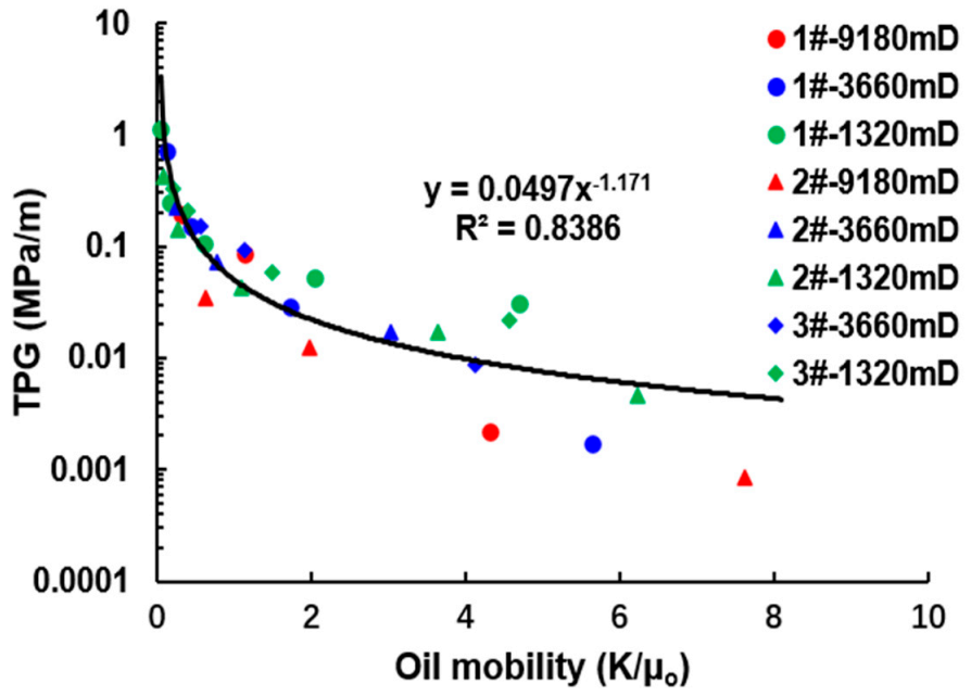
3.3. Threshold Pressure Gradient

Heavy oil could show the properties of the non-Newtonian fluid at low temperature. Yang et al. [37] and Wu et al. [21] established a productivity model of the CSS process, in which the TPG has been considered in the cold zone. It is commonly assumed that the TPG of heavy oil is related to oil viscosity and permeability. Sun [35] established an expression between oil mobility and the TPG by fitting experimental data. Figure 4 shows a typical correlation of the TPG for the unconsolidated sandstone heavy oil reservoirs, which varies with oil mobility. In this paper, this model will be used to describe the non-Newtonian flowing characteristics of heavy oil in a porous media.

3.4. Production Performance Model in a Multilayer Heavy Oil Reservoir

CSS is a pressure-declining recovery process. It indicates that the reservoir pressure decreases continuously with the fluid production. Therefore, a pseudo-steady state fluid flow model can be applied to estimate the production performance. Furthermore, the equivalent flow resistance principle is utilized to derive the production formula, in which the reservoir is composed of the cold zone, hot water zone, and steam zone.

For a particular thin layer reservoir, according to the theory of radial flow in the pseudo-steady state, its oil production rate can be expressed as,

$$Q_o(t_p,N,j)=\frac{0.0864\left(P_{avg}\left(t_p,N,j\right)-P_{wf}-TPG·\left(r_e-r_h\right)\right)}{B_o·R_o\left(t_p,N,j\right)}$$

(33)

The fluid flow resistance in the cold zone is,

$$R_{oc}\left(t_p,N,j\right) =\frac{{\mu }_{o\mathrm{c}}}{2\pi h_{j}K{K}_{roc}}\left(\ln \frac{r_e}{r_h}-\frac{3}{4}+\frac{r_h^2}{2r_e^2}\right)$$

(34)

Considering the temperature distribution in the hot water zone and the effects of temperature on the relative permeability curve and oil viscosity, the fluid flow resistance in the hot water zone can be expressed as,

$$R_{oh}\left(t_p,N,j\right) =\frac{1}{2\pi h_{j}K}{\displaystyle {\int }_{r_s}^{r_h}\frac{{\mu }_{oh}}{K_{roh}}\left(\frac{1}{r}-\frac{r}{r_e^2}\right)dr}$$

(35)

The fluid flow resistance in the steam zone is,

$$R_{os}\left(t_p,N,j\right) =\frac{{\mu }_{os}}{2\pi h_{j}K{K}_{ros}}\left(\ln \frac{r_s}{r_w}-\frac{r_s^2}{2r_e^2}+S\right)$$

(36)

According to the water-electricity similarity principle, the total oil phase seepage resistance can be expressed as,

$$R_o\left(t_p,N,j\right) =R_{oc}\left(t_p,N,j\right) + R_{oh}\left(t_p,N,j\right) + R_{os}\left(t_p,N,j\right)$$

(37)

Similarly, the water production rate can be expressed as,

$$Q_w(t_p,N,j)=\frac{0.0864\left(P_{avg}\left(t_p,N,j\right)-P_{wf}\right)}{B_w·R_w\left(t_p,N,j\right)}$$

(38)

3.5. The Evolution of Reservoir Dynamic Parameters

For the production rate formula of a particular thin layer reservoir, several dynamic parameters should be calculated, e.g., average reservoir pressure, average water saturation, average temperature, and cyclic residual heat. Furthermore, the oil viscosity and relative permeability can be obtained based on the corresponding viscosity-temperature correlation and oil-water relative permeability curve.

3.5.1. Average Reservoir Pressure

The injection of steam induces an increase in reservoir pressure, and the material balance equation can obtain it; the underground volume of injected steam equals the sum of the volume expansion of the pore and the volume compression of the reservoir fluids. The expression of the pressure at the end of the soaking period can be obtained by arranging the equation as follows,

$$P_{avg,s}=P_i+\frac{G_w·B_w}{N·B_o·C_e}+\frac{N_{os}·(T_{savg}-T_i)·{\beta }_e}{N·C_e}+\frac{N_{oh}·(T_{havg}-T_i)·{\beta }_e}{N·C_e}$$

(39)

The principle is also applied to the oil production period; the underground volume of the produced fluids equals the sum of the volume expansion of the reservoir fluids and the volume compression of the pore. The average reservoir pressure during the oil production process can be expressed as,

$$\begin{array}{l}{P}_{avg,p}=P_{avg,s}-\frac{N_w{B}_w+N_o{B}_o}{N·B_o·C_e}-\frac{N_{os}(T_{savg}-T_{as}(t_p,N,j))·{\beta }_e}{N·C_e}\\ -\frac{N_{oh}(T_{havg}-T_{ah}(t_p,N,j))·{\beta }_e}{N·C_e}\end{array}$$

(40)

in which the comprehensive thermal expansion coefficient and the compressibility coefficient of the reservoir are expressed as respectively,

$${\beta }_e={\beta }_o+\frac{{\beta }_w·S_{wi}}{S_{oi}}+\frac{{\beta }_r·(1-\varphi )}{\varphi ·S_{oi}}$$

(41)

$$C_e=C_o+\frac{C_w·S_{wi}}{S_{oi}}+\frac{C_p}{\varphi ·S_{oi}}$$

(42)

3.5.2. Average Water Saturation

According to the conservation equation for the aqueous phase, the average water saturation in the heated zone equals the initial water saturation and the saturation variation caused by steam injection and water production. It can be expressed as [11],

$$S_w=S_{wi}\frac{d_{wi}}{d_w}+\frac{G_w-N_w}{\phi \pi r_h^2{h}_j}$$

(43)

3.5.3. Cyclic Residual Heat

Generally, there is residual heat in the heated zone when a new CSS cycle begins. From the second CSS cycle, it is assumed that the reservoir remains at the initial temperature; thus, the calculation of the heating radius needs to combine the steam injection rate and the residual heat of the last cycle. The cyclic residual heat of the steam zone and the hot water zone can be expressed as respectively,

$$E_{rs}=\pi r_s^2{h}_j{M}_R\left(T_{as}(t_p,N,j)-T_i\right)$$

(44)

$$E_{rh}=\pi \left(r_h^2-r_s^2\right)h_j{M}_R\left(T_{ah}(t_p,N,j)-T_i\right)$$

(45)

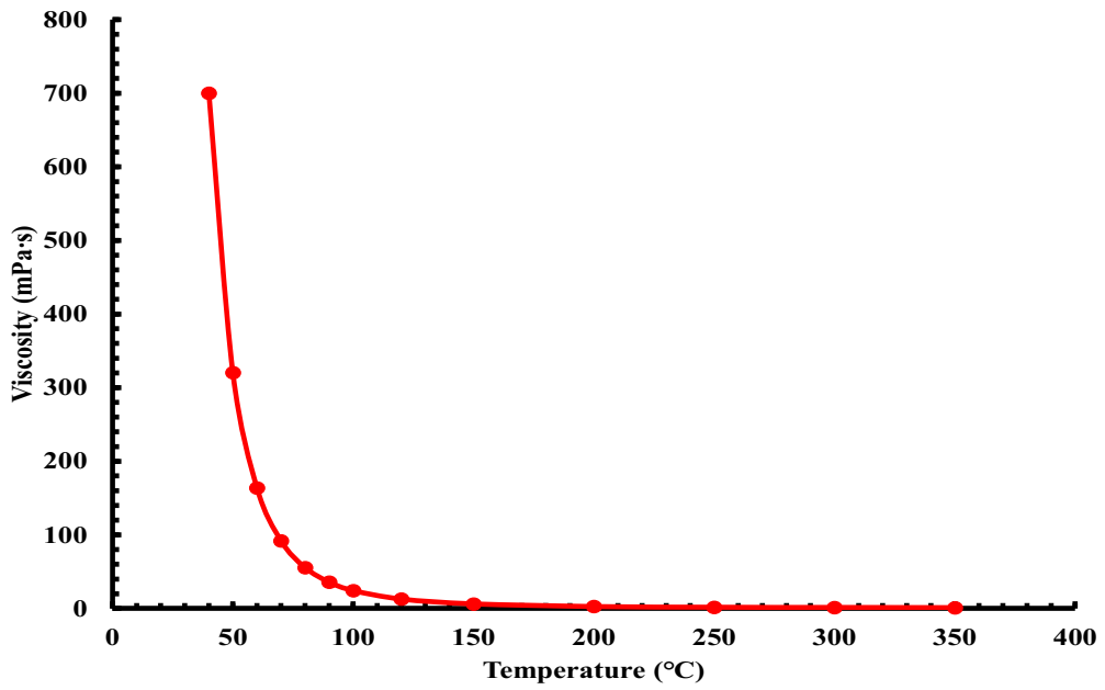
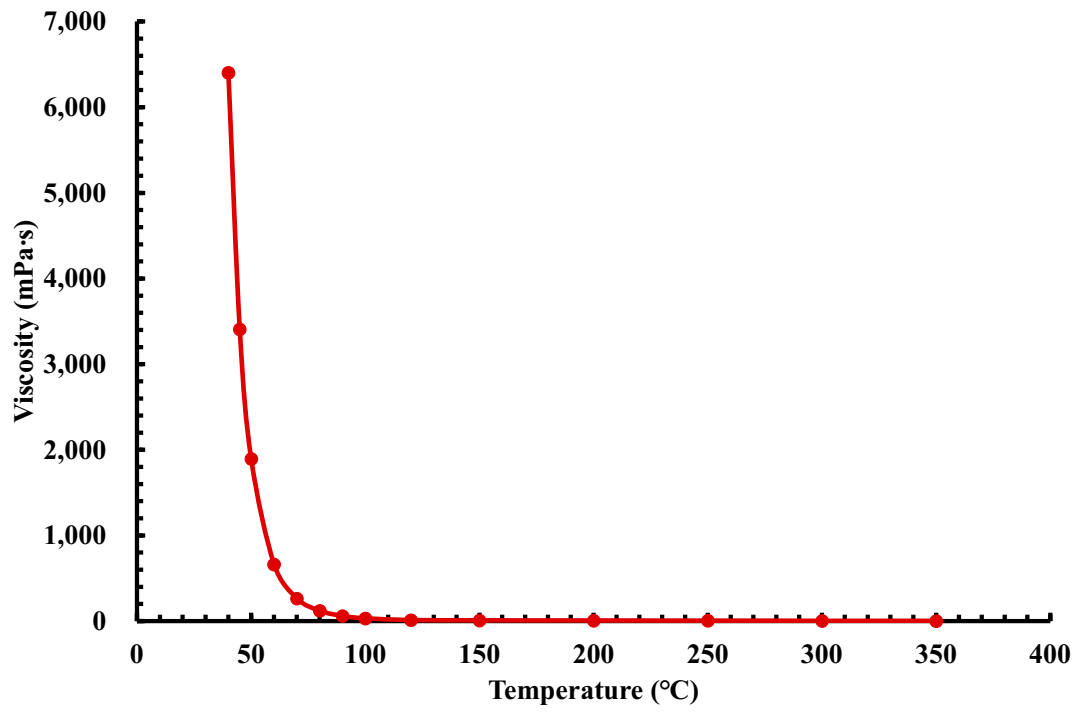
3.5.4. Oil Viscosity

Considering that the viscosity of heavy oil is usually given with a viscosity-temperature table, viscosity and temperature show a linear relation on the ASTM coordinate chart. Therefore, the viscosity at any temperature can be obtained by interpolation on the ASTM coordinate. The linear relation is as follows,

$$\lg \lg {\mu }_o=C-D\lg T$$

(46)

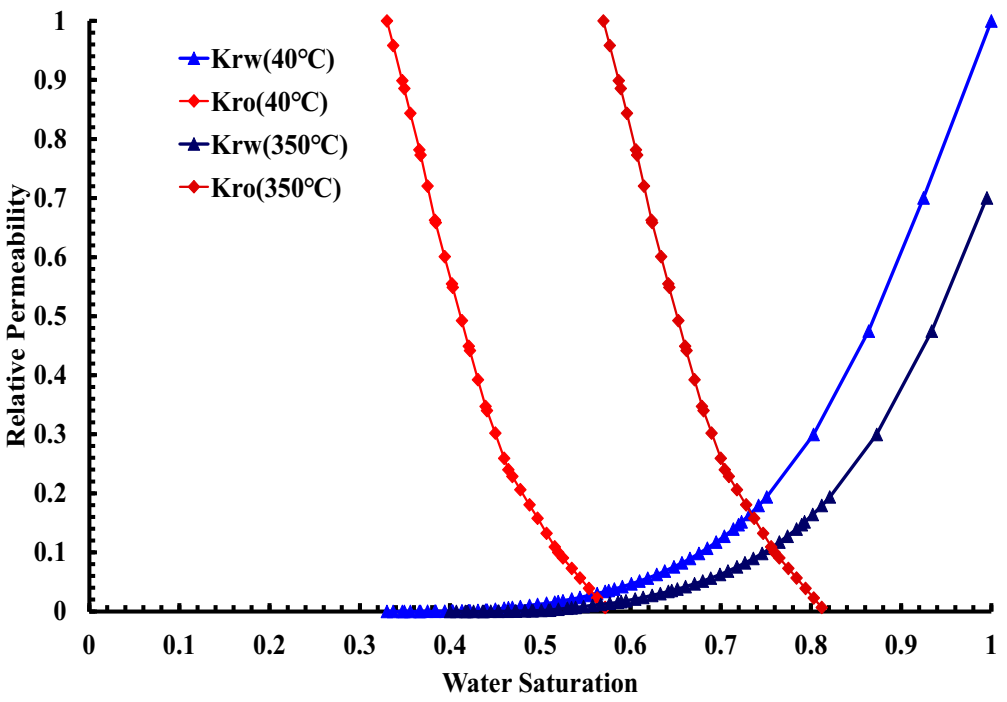
3.5.5. Oil-Water Relative Permeability Curve

The endpoints of the oil-water relative permeability curve are related to temperature, while the curve shape is similar at different temperatures. Meanwhile, the oil (water) relative permeability is a function of water saturation at a given temperature. For the CSS process, the procedure for determining oil-water relative permeability includes an interpolation of the oil (water) relative permeability at a specific temperature based on a given oil-water relative permeability table and shifting the curve based on the endpoints of different temperatures.

Thus, based on the above mathematical model, the productivity of the CSS well in a multilayer heavy oil reservoir can be obtained. Contrary to the previous published models, in our mode, the non-isothermal feature is considered. Specifically, the heated zone is comprised of a steam zone and a hot water zone. Simultaneously, the TPG effect is considered as a function of oil mobility, and the effect of the steam overlay is also considered.

3.6. Model Limitation

In Section 2, we assumed that the reservoir is homogeneous and isotropic. Another important assumption in our model is that the temperature in the hot water zone decreases linearly from the temperature in the steam zone to the initial reservoir temperature. Therefore, it indicates that for the heavy oil reservoirs with a serious permeability heterogeneity, our method is not available to predict the productivity of the CSS wells.

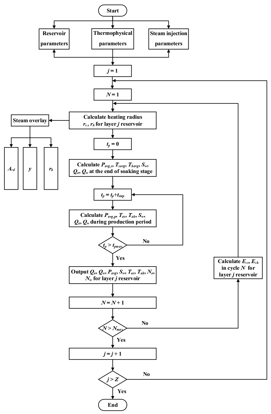
4. Calculation Procedure

The primary solution for the multilayer heavy oil reservoir production model consists of: determining the dynamic production data for a specific thin layer reservoir, e.g., the oil production rate, cumulative oil production, etc.; then, the data for the entire heavy oil reservoir can be obtained by synthesizing the data from all the formation layers. The detailed procedures are as follows:

(1) Inputting the required data, including the reservoir, thermophysical, and steam injection parameters.

(2) Splitting the amount of steam injected into each layer using the formation factor distribution method of Equation (1).

(3) Considering the steam overlay—the shape coefficient (A_rd), radius ratio (y), and heating radius of the underburden (r_b) are calculated in turn to determine the equivalent heating radius (r_s) in the steam zone using Equation (7).

(4) Calculating the heating radius (rh) in the hot water zone by Equation (10).

(5) Calculating the average reservoir pressure, the average temperature in the steam zone, the average temperature in the hot water zone, the average water saturation, etc. at the end of the soaking stage by Equations (39), (15), (24), and (43). The oil production and the water production can then be obtained by Equations (33) and (38).

(6) Similarly, calculating the average reservoir pressure, the average temperature in the steam zone, the average temperature in the hot water zone, the average water saturation, etc. during the oil production period by Equations (40), (18), (28), and (43); then, oil production and water production can be obtained by Equations (33) and (38).

(7) Calculating the cyclic residual heat in the heated zone by Equations (40) and (41), respectively. The production performance of the different CSS cycles in a specific thin layer reservoir can be determined by repeating steps (3)–(7).

(8) The production performance of the multilayer heavy oil reservoir can be determined by repeating steps (2)–(7).

The simulation diagram for the above calculation process is shown in Figure 5.

5. Results and Discussion

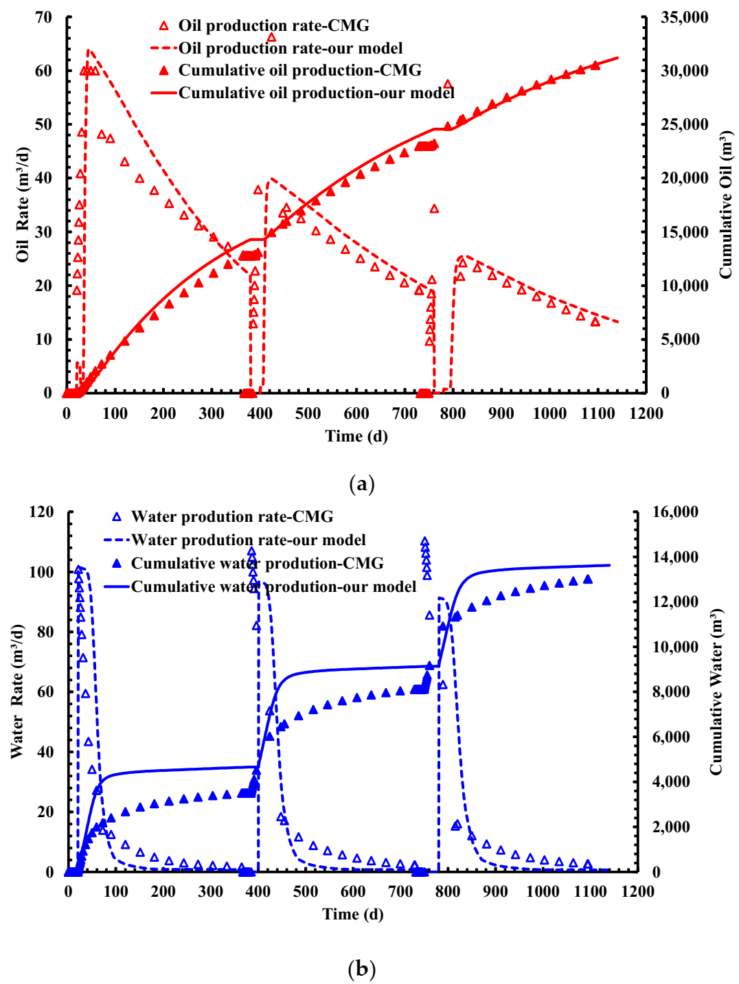
5.1. Model Validation

Based on the above model, the production performance of a CSS well in a multilayer heavy oil reservoir can be obtained. In this section, the calculation results of our model will be compared against the simulation results of CMG software to validate the accuracy of this mode. The basic parameters used in the validation process are taken from an actual CSS well in the Jinzhou 23-2 block, CNOOC, as shown in

Table 1. The basic parameters used in this study.

Stage	Parameters	Value
Basic parameters	Reservoir thickness, m	7.5 * 3 + 10 + 7.5
	Porosity, decimal	0.28
	Permeability, mD	1200
	Initial reservoir pressure, MPa	10
	Initial reservoir temperature, °C	40
	Initial water saturation, decimal	0.33
	Reservoir compressibility, MPa−1	0.0055
	Wellbore radius, m	0.1
	Bottom hole pressure, MPa	6
	Thermal conductivity of reservoir, kJ/(d·m·°C)	163.4
	Thermal conductivity of interlayers, kJ/(d·m·°C)	105.5
	Heat capacity of reservoir, kJ/(m3·°C)	2575
	Heat capacity of interlayers, kJ/(m3·°C)	2200
	Oil thermal expansion coefficient, °C−1	0.00045
	Water thermal expansion coefficient, °C−1	0.00015
	Oil specific heat capacity, kJ/(kg·°C)	2.1
	Water specific heat capacity, kJ/(kg·°C)	4.2
Steam injection parameters	Injection time, d	15
	Soaking time, d	5
	Production time, d	360
	CSS cycles, dless	3
	Steam injection rate, t/d	300
	Injection temperature, ·°C	340
	Steam quality, decimal	0.4

. The oil-water relative permeability curve and the oil viscosity-temperature curve, respectively, are shown in Figure 2 and Figure 3. The comparison results are shown in Figure 6. As shown, a good agreement can be observed. The changing trends of the different curves are well-matched, including the oil production and water production. For the oil production results, the entire changing trends are very close, especially for the last two CSS cycles. The relative error of the cumulative oil production within three CSS cycles is about 2.20%, and the relative error of the cumulative water production within three CSS cycles is about 4.69%. Therefore, this indicates that our new model can provide an accurate prediction for the productivity of a CSS well in multilayer heavy oil reservoirs.

5.2. Sensitivity Analysis

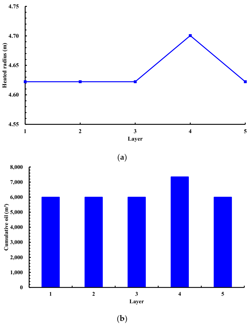
5.2.1. Effect of Formation Factor

The simulated heavy reservoir applied in this paper includes five formation layers. As shown in Table 1, the reservoir thickness of the fourth layer is the highest. It indicates that the formation factor is different for each layer. The calculation results for each layer are shown in Figure 7. As shown, compared with the reservoir thickness (7.5 m) of the other four layers, the thickness of the fourth layer is 10 m. According to the method of splitting the steam amount, the fourth layer has a higher steam injection volume. In addition, its heating radius is 0.08 m greater than that of other layers (Figure 7a). Obviously, both greater reservoir thickness and greater heating radius are inclined to improve oil production. Therefore, it yields an increase of 1347.6 m³ on the cumulative oil production for the fourth layer of the reservoir.

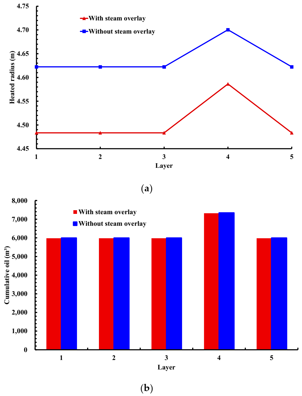
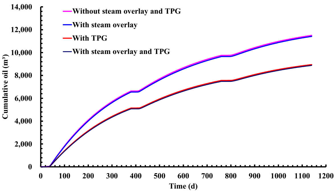
5.2.2. Effect of Steam Overlay

Under the effect of the steam overlay, the steam will rise toward the reservoir top after it is injected into the reservoir. Currently, for the condition considering the effects of the steam overlay, a commonly-used method is based on van Lookeren’s theory [21]. From this theory, the shape coefficient and the radius ratio can be easily obtained. Then, the equivalent heating radius with the effect of the steam overlay in the steam zone can be calculated. Thus, the oil production rate and the cumulative oil production can be calculated. For the first CSS cycle, the detailed comparison of the equivalent heating radius and the cumulative oil production for the five formation layers are shown in Figure 8. As shown, for the case with the effect of the steam overlay, the heating radius is reduced by 0.14 m less than the other cases. Nevertheless, for the cumulative oil production, a slight distinction can be observed (see Figure 8b). Specifically, for the fourth layer, compared with the case without the effect of the steam overlay, the cumulative oil production is reduced by about 24 m³. This indicates that in a field application, the effect of the steam overlay is negligible.

5.2.3. Effect of Threshold Pressure Gradient (TPG)

Contrary to previous publications, in this paper, the TPG of the heavy oil is considered as a function of oil mobility, as shown in Figure 4. It indicates that the TPG of heavy oil is related to the formation permeability and oil viscosity. From Equation (33), it can be found that the consideration of the TPG will further reduce the effective pressure drop, and thus the oil production rate will be reduced. Figure 9 gives the calculation results with and without the consideration of the TPG. As shown, for the fourth formation layer, once the effect of the TPG is considered, the cumulative oil production will be decreased from 7382.1 m³ to 7312.9 m³. Thus, it can be seen that the difference is around 0.94%, and the effect of the TPG in this case can be neglected as well. Based on the TPG expression in Figure 4 and the oil viscosity in Figure 3, it can be determined that the oil viscosity is relatively low. Thus, a low TPG can be obtained.

In order to further demonstrate the effect of the steam overlay and the TPG, a new oil viscosity-temperature is selected, as shown in Figure 10. Compared with the previous oil viscosity (see Figure 3), a higher oil viscosity is applied in this case. Thus, by using the new oil viscosity, the cumulative oil production can be re-calculated, as shown in Figure 11. A significant difference can be observed. Because of the increase in oil viscosity, the TPG is increased, and thus the oil production rate is highly reduced. Simultaneously, compared with the steam overlay, the effect of the TPG is more significant. Compared with the simulation case, where both the effect of steam overlap and the TPG are neglected, the cumulative oil deviations caused by the steam overlap and the TPG are at around 80 m³ and 2500 m³, respectively.

5.2.4. Effect of Bottom Hole Pressure

Bottom hole pressure (BHP) is another important parameter that can significantly affect the oil production rate. In a field operation, changing the bottom hole pressure is a commonly used method for adjusting the oil production rate. In this section, the effect of bottom hole pressure on the recovery performance of the CSS well is simulated. The results are shown in Figure 12. As shown, as the BHP reduces, the pressure difference is increased, thus increasing the oil production rate. From Table 1, in this case, the initial reservoir pressure is 10 MPa. Thus, from Figure 12, it can be noted that as the BHP is reduced from 6 MPa to 4 MPa, the cumulative oil production will be increased from 30,987 m³ to 45,668 m³, indicating that a 2 MPa increase in pressure difference can increase the cumulative oil production by about 47% within three CSS cycles.

6. Summary and Conclusions

(1) A new production performance model for the cyclic steam stimulation process in multilayer heavy oil reservoirs is established in this paper. In order to consider the issue of multilayer formation, the parameter of the formation factor is applied to split the steam volume of each formation layer. Simultaneously, this model fully considers the effect of the steam overlay and the TPG. Contrasting with the previous models, the TPG model used in our method is a function of oil mobility. It can accurately reflect the non-Newtonian flow behavior of the heavy oil in porous media.

(2) By using the reservoir and fluid properties of an actual CSS well, the simulation results of our model are compared against the results of the CMG software to validate this model. A good agreement is observed, indicating that this model can accurately reflect the recovery performance of the CSS process in multilayer heavy oil reservoirs.

(3) A sensitivity analysis is conducted to discuss the effect of different factors (formation factor, steam overlay, TPG, and BHP) in multilayer heavy oil reservoirs. The results indicate that the effect of the steam overlay on the production process can be neglected. The consideration of the steam overlay slightly reduces the heating radius and the cumulative oil production. Comparatively, the effect of the TPG is higher, but it depends on the oil viscosity. A higher oil viscosity can indicate a higher TPG, and thus the TPG effect is enhanced.

References

1. Liu, H. Thermal Recovery Principle and Method; Petroleum Industry Press: Beijing, China, 2013. [Google Scholar]
2. Dong, X.; Liu, H.; Chen, Z.; Wu, K.; Lu, N.; Zhang, Q. Enhanced oil recovery techniques for heavy oil and oilsands reservoirs after steam injection. Appl. Energy 2019, 239, 1190–1211. [Google Scholar] [CrossRef]
3. Thomas, S. Enhanced oil recovery-an overview. Oil Gas Sci. Technol. Rev. IFP 2008, 63, 9–19. [Google Scholar] [CrossRef] [Green Version]
4. Hou, J.; Sun, J. Thermal Recovery Techniques; China University of Petroleum Press: Dongying, China, 2013. [Google Scholar]
5. Somerton, W.H.; Keese, J.A.; Chu, S.L. Thermal behavior of unconsolidated oil sands. SPE J. 1974, 14, 513–521. [Google Scholar] [CrossRef]
6. Thanh, H.V.; Sugai, Y.; Nguele, R.; Sasaki, K. Robust optimization of CO2 sequestration through a water alternating gas process under geological uncertainties in Cuu Long Basin, Vietnam. J. Nat. Gas Sci. Eng. 2020, 76, 103208. [Google Scholar] [CrossRef]
7. Li, B.; Zhang, J.; Kang, X.; Zhang, F.; Wang, S.; Zhao, W.; Wang, X.; Wei, Z. Review and prospect of the development and field application of China offshore chemical EOR technology. In Proceedings of the Abu Dhabi International Petroleum Exhibition & Conference, Abu Dhabi, United Arab Emirates, 11–14 November 2019. [Google Scholar]
8. Tang, X.; Ma, Y.; Sun, Y. Research and field test of complex thermal fluid huff and puff technology for offshore viscous oil recovery. China Offshore Oil Gas 2011, 23, 185–188. [Google Scholar]
9. Li, P.; Liu, Z.; Zou, J.; Liu, H.; Yu, J.; Fan, Y. Injection and production project of pilot test on steam huff-puff in oilfield LD27-2 Bohai Sea. Acta Pet Sin. 2016, 37, 242–247. [Google Scholar]
10. Li, X.; Zhang, F.; Huang, K.; Cui, D.; Huang, Y.; Miao, F. Discussion about the thermal recovery of NB35-2 offshore heavy oilfield. Reserv. Eval. Dev. 2011, 1, 61–63. [Google Scholar]
11. Boberg, T.C.; Lantz, R.B. Calculation of the production rate of a thermally stimulated well. J. Pet. Technol. 1966, 18, 1613–1623. [Google Scholar] [CrossRef]
12. He, C.G.; Mu, L.X.; Xu, A.Z.; Fang, S.D. A new model of steam soaking heating radius and productivity prediction for heavy oil reservoirs. Acta Pet. Sin. 2015, 36, 1564–1570. [Google Scholar]
13. Marx, J.W.; Langenheim, R.H. Reservoir heating by hot fluid injection. Trans. AIME 1959, 216, 312–315. [Google Scholar] [CrossRef]
14. Willman, B.T.; Valleroy, V.V.; Runberg, G.W.; Cornelius, A.J.; Powers, L.W. Laboratory studies of oil recovery by steam injection. J. Pet. Technol. 1961, 13, 681–690. [Google Scholar] [CrossRef]
15. Mandl, G.; Volek, C.W. Heat and mass transport in steam-drive processes. SPE J. 1969, 9, 59–79. [Google Scholar] [CrossRef]
16. Jones, J. Cyclic steam reservoir model for viscous oil, pressure depleted gravity drainage reservoirs. In Proceedings of the SPE 6544, paper presented at California Regional Meeting, Bakersfield, CA, USA, 13–15 April 1977. [Google Scholar]
17. Gros, R.P.; Pope, G.A.; Lake, L.W. Steam soak predictive model. In Proceedings of the SPE Annual Technical Conference and Exhibition, Las Vegas, NV, USA, 22–26 September 1985. [Google Scholar]
18. Li, C.; Yang, B. Non-isothermal productivity predicting model of heavy crude oil exploited with huff and puff. Oil Drill. Prod. Technol. 2003, 25, 89–90. [Google Scholar]
19. Hou, J.; Wei, B.; Du, Q.; Wang, J.; Wang, Q.; Zhang, G. Production prediction of cyclic multi-thermal fluid stimulation in a horizontal well. J. Pet. Sci. Eng. 2016, 146, 949–958. [Google Scholar] [CrossRef]
20. Zhang, Q.; Liu, H.; Kang, X.; Liu, Y.; Dong, X.; Wang, Y.; Liu, S.; Li, G. An investigation of production performance by cyclic steam stimulation using horizontal well in heavy oil reservoirs. Energy 2021, 218, 119500. [Google Scholar] [CrossRef]
21. Wu, Z.; Liu, H.; Zhang, Z.; Wang, X. A novel model and sensitive analysis for productivity estimate of nitrogen assisted cyclic steam stimulation in a vertical well. Int. J. Heat Mass Transf. 2018, 126, 391–400. [Google Scholar] [CrossRef]
22. Van Lookeren, J. Calculation methods for linear and radial steam flow in oil reservoirs. SPE J. 1983, 23, 427–439. [Google Scholar] [CrossRef]
23. Hou, J.; Chen, Y. An improved steam soak predictive model. Pet. Explor. Dev. 1997, 24, 53–56. [Google Scholar]
24. Lai, L.; Pan, T.; Qin, Y. A calculation method for heat loss considering steam overlap in steam flooding. J. Northwest Univ. 2014, 44, 104–110. [Google Scholar]
25. Tian, Y.; Ju, B.; Hu, J. A productivity prediction model for heavy oil steam huff and puff considering steam override. Pet. Drill. Tech. 2018, 46, 100–116. [Google Scholar]
26. Sun, F.; Li, C.; Cheng, L.; Huang, S.; Zou, M.; Sun, Q.; Wu, X. Production performance analysis of heavy oil recovery by cyclic superheated steam stimulation. Energy 2017, 121, 356–371. [Google Scholar] [CrossRef]
27. He, C.; Xu, A.; Fan, Z.; Zhao, L.; Zhang, A.; Shan, F.; He, J. An integrated heat efficiency model for superheated steam injection in heavy oil reservoirs. Oil Gas Sci. Technol. Rev. IFP Energ. Nouv. 2019, 74. [Google Scholar] [CrossRef]
28. Thomas, L.K.; Katz, D.L.; Tek, M.R. Threshold pressure phenomena in porous media. SPE J. 1968, 8, 174–184. [Google Scholar] [CrossRef]
29. Wu, Y.; Pruess, K.; Witherspoon, P.A. Flow and displacement of Bingham non-Newtonian fluids in porous media. SPE Reserv. Eng. 1992, 7, 369–376. [Google Scholar] [CrossRef] [Green Version]
30. Wang, S.; Huang, Y.; Civan, F. Experimental and theoretical investigation of the Zaoyuan field heavy oil flow through porous media. J. Pet. Sci. Eng. 2006, 50, 83–101. [Google Scholar] [CrossRef]
31. Tian, J.; Xu, J.; Cheng, L. The method of characterization and physical simulation of TPG for ordinary heavy oil. J. Southwest Pet. Univ. Sci. Technol. Ed. 2009, 31, 158–162. [Google Scholar]
32. Liu, H.; Wang, J.; Xie, Y.; Ma, D.; Shi, X. Flow characteristics of heavy oil through porous media. Energy Sources Part A Recovery Util. Environ. Eff. 2011, 34, 347–359. [Google Scholar] [CrossRef]
33. Dong, X.; Liu, H.; Wang, Q.; Pang, Z.; Wang, C. Non-Newtonian flow characterization of heavy crude oil in porous media. J. Pet. Explor. Prod. Technol. 2013, 3, 43–53. [Google Scholar] [CrossRef] [Green Version]
34. Huang, T.; Ning, Z.; Liu, H.; Zhang, S.; Xiao, L. Experiment investigation on mobility characteristics of different components of heavy oil. Sci. Technol. Eng. 2013, 13, 6851–6854. [Google Scholar]
35. Sun, J. Experimental Study on Single Phase Flow in Block Zheng 411 of Shengli Ultra Heavy Oil Reservoir. Drill. Pet. Tech. 2011, 39, 86–90. [Google Scholar]
36. Zhang, D.; Peng, J.; Gu, Y.; Leng, Y. Experimental study on threshold pressure gradient of heavy oil reservoir. Xinjiang Pet. Geol. 2012, 33, 201–204. [Google Scholar]
37. Yang, J.; Li, X.; Chen, Z.; Tian, J.; Huang, L.; Liu, X. A productivity prediction model for cyclic steam stimulation in consideration of non-Newtonian characteristics of heavy oil. Acta Pet. Sin. 2017, 38, 84–90. [Google Scholar]
38. Huang, S.; Kang, B.; Cheng, L.; Zhou, W.; Chang, S. Quantitative characterization of interlayer interference and productivity prediction of directional wells in the multilayer commingled production of ordinary offshore heavy oil reservoirs. Pet. Explor. Dev. 2015, 42, 533–540. [Google Scholar] [CrossRef]
39. Shen, F.; Cheng, L.; Sun, Q.; Huang, S. Evaluation of the vertical producing degree of commingled production via waterflooding for multilayer offshore heavy oil reservoirs. Energies 2018, 11, 2428. [Google Scholar] [CrossRef] [Green Version]
40. Dong, X.; Liu, H.; Chen, Z. Hybrid Enhanced Oil Recovery Processes for Heavy Oil Reservoirs. In Developments in Petroleum Science; Elsevier: Amsterdam, The Netherlands, 2021. [Google Scholar]
Figure 1. A schematic diagram of a multilayer heavy oil reservoir; (a) conventional mode; (b) our mode.
Energies 15 01757 g001
Figure 2. Oil-water relative permeability at different temperatures.
Energies 15 01757 g002
Figure 3. Oil viscosity vs. temperature.
Energies 15 01757 g003
Figure 4. The relationship between the TPG and oil mobility [40].
Energies 15 01757 g004
Figure 5. A flowchart for the calculation process of this model.
Energies 15 01757 g005
Figure 6. Simulation results—(a) Oil production rate and cumulative oil production; (b) Water production rate and cumulation water production.
Energies 15 01757 g006
Figure 7. Simulation results for different formation layers—(a) Heating radius; (b) Cumulative oil production.
Energies 15 01757 g007
Figure 8. Calculation results on the effect of the steam overlay—(a) Heating radius; (b) Cumulative oil production.
Energies 15 01757 g008
Figure 9. Calculation results on the effect of the TPG.
Energies 15 01757 g009
Figure 10. The viscosity-temperature curve of a higher oil viscosity.
Energies 15 01757 g010
Figure 11. The effect of the steam overlay and TPG on the cumulative oil production.
Energies 15 01757 g011
Figure 12. The effect of bottom hole pressure.
Energies 15 01757 g012