Article

Analyzing Europe’s Biggest Offshore Wind Farms: A Data Set with 40 Years of Hourly Wind Speeds and Electricity Production

Institute for Operations Research, Karlsruhe Institute of Technology (KIT), Kaiserstraße 12, 76131 Karlsruhe, Germany
*
Author to whom correspondence should be addressed.
These authors contributed equally to this work.
Energies 2022, 15(5), 1700; https://doi.org/10.3390/en15051700
Submission received: 24 January 2022 / Revised: 17 February 2022 / Accepted: 21 February 2022 / Published: 24 February 2022
(This article belongs to the Special Issue Economics of Offshore Wind Energy)

Abstract

:
We provide an open, available, and ready-to-use data set covering 40 years of hourly wind speeds and synthetic hourly production signals for the 29 biggest offshore wind farms in Europe. It enables researchers and industry experts to include realistic offshore time series into their analyses. In particular, we provide data from 1980 to 2019 for wind farms already in operation and those that will be in operation by 2024. We document in detail how the data set was generated from publicly available sources and provide manually collected details on the wind farms, such as the turbine power curves. Correspondingly, the users can easily keep the data set up to date and add further wind farm locations as needed. We give a descriptive analysis of the data and its correlation structure and find a relatively high volatility and intermittency for single locations, with balancing effects across wind farms.

1. Introduction

The EU has the largest wind energy exploitable maritime space in the world. Consequently, to reduce net greenhouse gas emissions, the EU plans to expand the current offshore wind capacity of 12 GW to 60 GW by 2030 and 300 GW by 2050 [1,2]. Similarly, the United Kingdom aims at reach 40 GW offshore wind capacity by 2030 in their Ten-Point Plan [3].
The main potential for such offshore wind farms in the EU and UK is located in the North Sea, due to relatively steadily blowing winds and shallow sea depths allowing for ground-based installations (see, e.g., [1,4,5] for recent studies). Accordingly, the vast majority of the 29 largest European offshore wind farms displayed in Figure 1 are located in the North Sea (further details in Section 2). In this context, data from wind farms are of particular interest for quantitative analyses related to the growing offshore capacities at these and nearby locations. Such data could feed to simulations, forecasts, models, or studies on the overall energy system. However, to the best of our knowledge, no such data are freely available to a broad public.
In this paper, we provide an hourly data set covering the last 40 years for the 29 biggest wind farms in Europe. We include wind speeds at hub height based on meteorological reanalysis data and further weather parameters as well as specifications of currently installed and planned wind turbines with parametric forms of their power curves. Furthermore, we provide synthetic energy time series of produced power over the considered horizon, i.e., power that would have been produced in the past at the respective locations with the current capacity and technology installed. These synthetic time series do not consider interactions of the installed turbines on their respective output, such as wake effects, or constraints in the connected power grids. The data set mainly focuses on the meteorological effects of electricity production. However, we include variables such as wind direction and surface roughness that allow enriching the potential of the data set for energy production analysis in future studies.
Studies in which data sets similar to ours could contribute can be found in the area of economic analysis (see, e.g., [6,7,8,9,10]) or grid integration ([11,12,13,14,15,16,17,18,19]) as well as in climate change analysis [20,21,22]. Among these papers, ref. [19] implicitly use a data set similar to ours to analyze future developments of an offshore (and energy) transmission grid in 2050. They consider 16 wind farms in the North Sea region and use a single reference wind turbine to calculate future feed-in data from meteorological reanalysis data, taking wake effects into account. A recent publication providing a short overview over calculation feed-in data from reanalysis data is [23] (see also the references therein). Further contributions methodologically related to ours include [24], who uses among other data high-resolution geo-spatial wind speed data to analyze renewable energy potentials in the European Union. In addition, the work of [25] synthetically calculates Swedish wind power production based on a single reference turbine for three years. With respect to modeling spatial and temporal dependency structures of wind power production, ref. [26] analyzed northern European countries and waters. For onshore locations, recent studies related to ours include, e.g., [27,28,29,30,31].
The data set provided in our paper can be of particular use and interest to researchers and industry experts as well as policymakers. It is prepared in a structured way so that a broad readership can analyze the data without much computational skills and effort. To better understand the data and potential insights derived from it, we give a first analysis. We include descriptive statistics and aggregate production figures over various time horizons for each wind farm as well as for total electricity production. This includes average production numbers, full load hours, and numbers for site-specific volatility and intermittency. By calculating these variables, we obtain an overview of all wind farms and the possibility to compare production characteristics at different locations. Since offshore wind energy is intended to play an essential role in the future European power system, we further analyze the dependencies of wind speed and electricity production between considered locations. Such analysis is interesting and very relevant with respect to reducing the wind power variability by aggregating productions from diverse geographical locations. While highly correlated locations lead to high volatility and intermittency in the overall supply, low correlations balance the overall output. Interestingly, the correlations of offshore wind farms over distance behave similarly to those found in onshore studies [32,33,34] but show higher correlations in neighboring locations.
The remainder of the paper is structured as follows. The data published with this paper, including weather data, information about wind farms, and derived wind power generation, are presented in Section 2. We explain the data generation step by step so that readers can keep the data set updated and extend it according to their needs. Section 3 includes the results of the analysis of the 29 wind farms. It is divided into a descriptive analysis for all of them as well as combined and a dependence analysis. We conclude in Section 4.

2. Data

We provide 40 years of hourly wind and production data for Europe’s 29 largest offshore wind farms in terms of installed capacity. The data include wind farms that are still under construction but will begin commercial operation in the next three years (by 2024). The locations of these farms are shown in Figure 1 and listed with technical details in Table 1. Our data set consists of hourly wind speeds and synthetic hourly power generation signals for each site. Wind speeds were determined by matching the wind farms locations to the nearest grid point in the ERA5 data set [35] and transforming the wind speeds at 100 m to the hub heights of the turbines. Afterwards, the wind speeds were converted to production signals using the power transfer function of each turbine, which we also provide in this paper. All steps are explained in detail below.
Details about the considered wind farms in Table 1 include their approximate location, hub height (Hub (m)), turbine types, resulting capacity in MW, and the start of commercial operations. The location of each wind farm is rounded to the next quarter longitude and latitude; thus, the positions are projected to a grid corresponding to the resolution of the weather data described below. Lastly, we assign a letter to each wind farm for improved visualization.
Baseline data of each wind farm were manually collected from publicly available information given by the operator of each wind farm or other public information (see Table A1 in Appendix A). Note that although we are talking about 29 wind farms, the number is not so clear to define, and one could, turning to Table 1, also talk about 28 or 32 considered parks. For example, we count Horns Rev Phase 1–3, a wind project built from three turbines types, as one wind farm, since the three parts map onto the same weather coordinates. Opposed to that, we count, e.g., the two projects Hollandse Kust Zuid/Noord as two wind farms. So, decisive for us are the resulting locations we are able to distinguish in the network of weather data.
For the weather data, we extract ERA5 data for every wind farm location from the Copernicus Climate Change Service (C3S) Climate Data Store (CDS) [35]. There, the weather data are provided on a grid of quarter degrees in longitude and latitude, and thus, we already matched each wind farm to the nearest grid point in Table 1. For each location, we extract the lateral wind speed components u and v in (m/s) at 100 m above ground. We neglect the lateral wind component and compute the absolute wind speed s p e e d 100 from these two orthogonal components, by
s p e e d 100 = u 2 + v 2
and wind direction ϕ by
ϕ = 180 π mod π + atan 2 ( v , u ) , 2 π ,
where we have ϕ = 0 for a northerly wind and the angle increases clockwise. Here, atan2 is the 2-argument arctangent function.
In the subsequent step, we follow [32,36] and assume a logarithmic velocity profile to scale the wind speeds s p e e d h u b to different hub heights h h u b (in m) of the turbines based on [37]:
s p e e d h u b = s p e e d 100 * ( l o g ( 100 ) l o g ( z 0 ) l o g ( h h u b ) l o g ( z 0 ) ) .
Here, z 0 corresponds to the surface roughness depending on the actual ocean state (characteristic height of waves, depth, etc.), which is also provided in the ERA5 data set [35]. For wind farms with unknown hub height (where we did not manage to find reliable information, nor were able to calculate it, see Table 1), we set the hub height to 100 m.
Figure 2 displays the wind roses of wind in 100 m for wind farms Gwynt y Mor and Kriegers Flak. Note that Gwynt y Mor represents the most western wind farm in our data, and Kriegers Flak represents the most eastern.
Despite the notable difference in their position, the resulting wind roses indicate quite similar main wind directions for both wind farms and very few northern as well as north-eastern winds. However, we observe a higher proportion of low wind speed hours at the Gwynt y Mor wind farm, which is located in a bay of the Irish Sea near the shore (wind farm C in Figure 1). This difference will also be visible in the descriptive statistics of generated power in Section 3, where, e.g., we observe more downtimes of Gynt y Mor due to low winds (below 4 m/s, which is typically the cut-in speed) compared to the Kriegers Flak wind farm.
As a final step in data preparation, we convert the wind speed data into synthetic power output using the turbines’ power curves. However, in the datasheets of most turbine types, the power curve is only given for individual points, i.e., in the form of a table with discrete wind speeds and corresponding nominal output power. We follow [38] and fit a combination of third-order polynomials to the nominal power at each wind speed to get a functional relationship. A piece-wise definition of the function is given by
p ( s p e e d h ) = 0 , i f s p e e d h u b < s p e e d m i n α 1 s p e e d h u b + β 1 s p e e d h u b + γ 1 s p e e d h u b + δ 1 , i f s p e e d m i n < s p e e d h u b < s p e e d s p l i t α 2 s p e e d h u b + β 2 s p e e d h u b + γ 2 s p e e d h u b + δ 2 , i f s p e e d s p l i t < s p e e d h u b < s p e e d r a t e d p r a t e d , i f s p e e d r a t e d < s p e e d h u b < s p e e d m a x 0 , i f s p e e d m a x < s p e e d h u b ,
where for each turbine type, s p e e d m i n is the cut-in speed, i.e., the minimum wind speed required for any power, and s p e e d r a t e d is the minimum wind speed for the rated power. s p e e d m a x is defined as cut-out speed, i.e., the speed at which the turbine is stopped or braked, and set to s p e e d m a x = 25 m/s for all turbines. In addition to these technical parameters of the turbines, s p e e d s p l i t is the turning point within our functional representation, where we change to the second polynomial. As proposed by [38], we fitted a third-order polynomial to find this point, where the concavity of the power curve changes sign. The resulting power curves for the wind turbine Siemens SWT-3.6-107 and Siemens Gamesa SG 8.0-167 DD, installed in wind farms Gwynt y Mor and Kriegers Flak, are shown in Figure 3.
Fitted polynomials and plots for the other turbine types are given in Appendix C. Note that data on nominal power at different wind speeds were not available for four turbines (Vestas V164-8.25, V164-9.0, V164-10.0, and Siemens Gamesa SG 11.0-200 DD). In these cases, we used a scaled version of the most similar Vestas V164-9.5 power curve instead. To be more specific about the scaling, consider, e.g., an unknown turbine with a nominal capacity of 8 MW and an unknown power curve. Then, the unknown power curve is approximated by adopting the shape of the 9.5 MW Vestas V164-9.5 turbine, and each value is scaled by 8 9.5 .
Having a time series of power output of every single turbine at each wind farm, we sum up all turbines belonging to the same wind farm to model the farms’ overall resulting power output. Without a doubt, this aggregation is a simplification of the actual effects of how individual wind turbines combine to form a wind farm. However, it suffices to provide insights into overall variations, intermittencies, their time constants, as well as distributional characteristics of power production at certain locations and dependency patterns between locations. For studies where the absolute level of generated power of particular wind farms is needed as accurately as possible, we recommend taking the interactions of the wind turbines such as wake effects into account. An implicit way of doing that would be by calibrating the synthetic power data calculated here with the help of measured power data over a short period of time. Depending on the amount of measured data available, one could use different calibrations for different wind conditions such as wind direction or light wind and strong wind scenarios. Alternatively, one could try to consider wake effects within the aggregation step using a theoretical model that incorporates relevant parameters about the wind farm’s outline. Various approaches to model these effects have been proposed, and detailed overviews are given, e.g., in [39,40,41].
The resulting total produced electricity of the Gwynt y Mor and Kriegers Flak wind farms in 2019 is displayed in Figure 4a,b for illustration. The figure shows that the power outputs at these locations are highly volatile and vary between no output at all and the maximum, i.e., the rated power. For better visualization, Figure 5 gives a more detailed view of Gwynt y Mor for January 2019. Here, flat tableaus where the wind speed falls below the cut-in speed or exceeds the speed of rated power are visible. The high volatility of the series might not be surprising for readers familiar with offshore wind power, but it clearly shows that the idea of the wind blowing continuously on the sea is not accurate. However, turning back to Figure 4, we can observe that the upper/lower bound of the power output is often reached at different points in time and, consequently, we expect that aggregating the power from multiple sites will have a flattening effect on the overall production.
We end this section with an overview of the exact format in which we provide the data set before we give a brief (descriptive) analysis in the next section. The data set may be downloaded as a zip archive under the provided DOI. It consists of 31 CSV files, one for each wind farm (total 29), one file summarizing the wind speed, and one for the resulting power outputs. In the first 29 files, we report detailed data for each wind farm, including wind components u and v, the forecast surface roughness (fsr), calculated wind speed, wind direction, scaled wind speed at hub height, and estimated power for each turbine type in the columns. Similar to the last two files, reporting wind speed at hub height and total power for each wind farm, each row represents one point in time. Starting from 1 January 1980, 00:00 a.m. UTC in the first row, the data set ranges up to 31 December 2019, 11:00 p.m. in the last of 350,640 rows.

3. Analysis

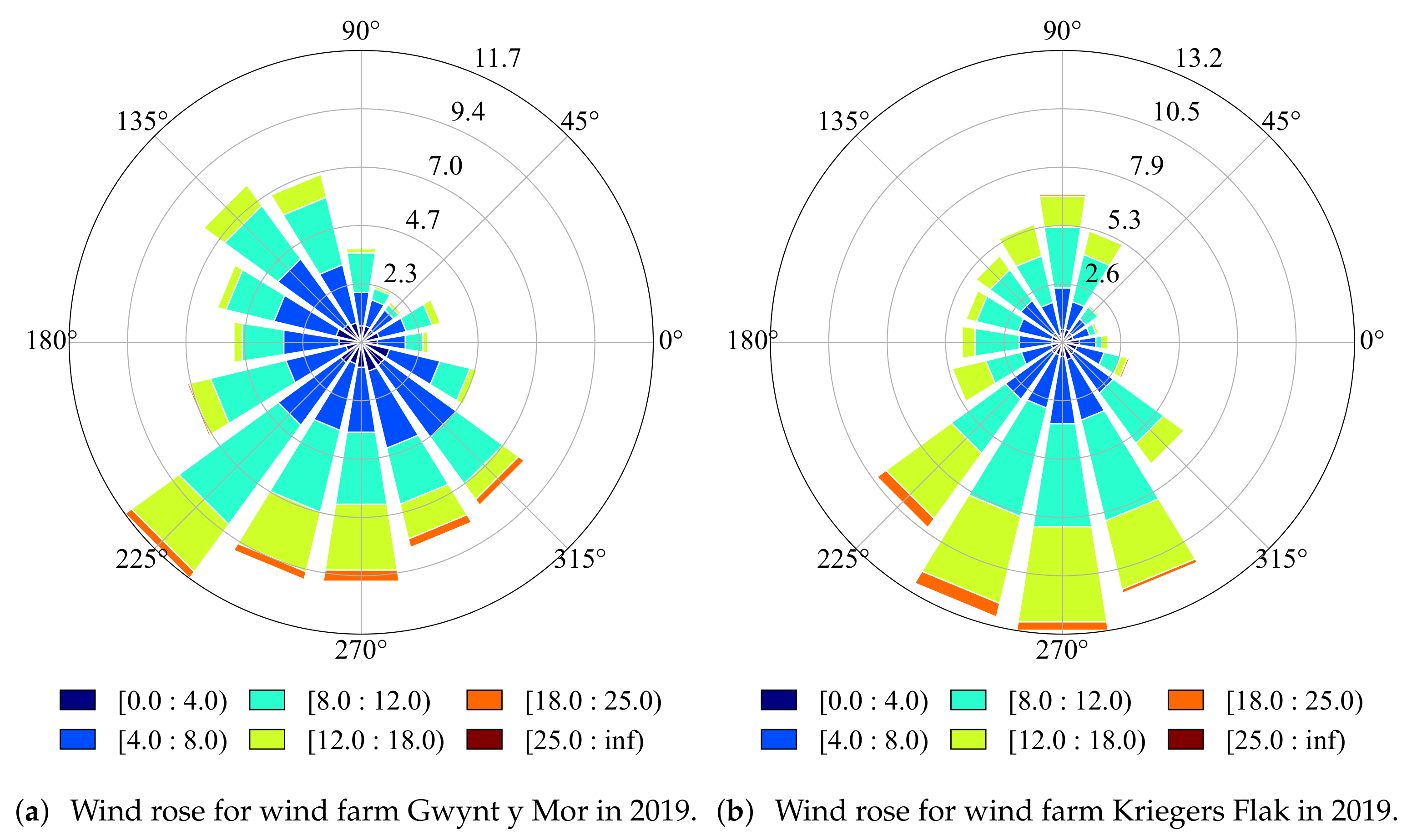
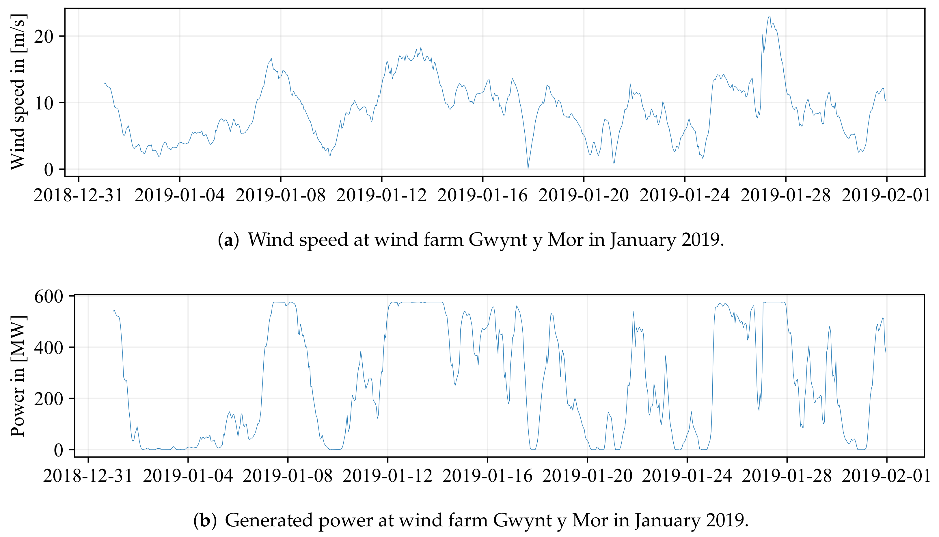
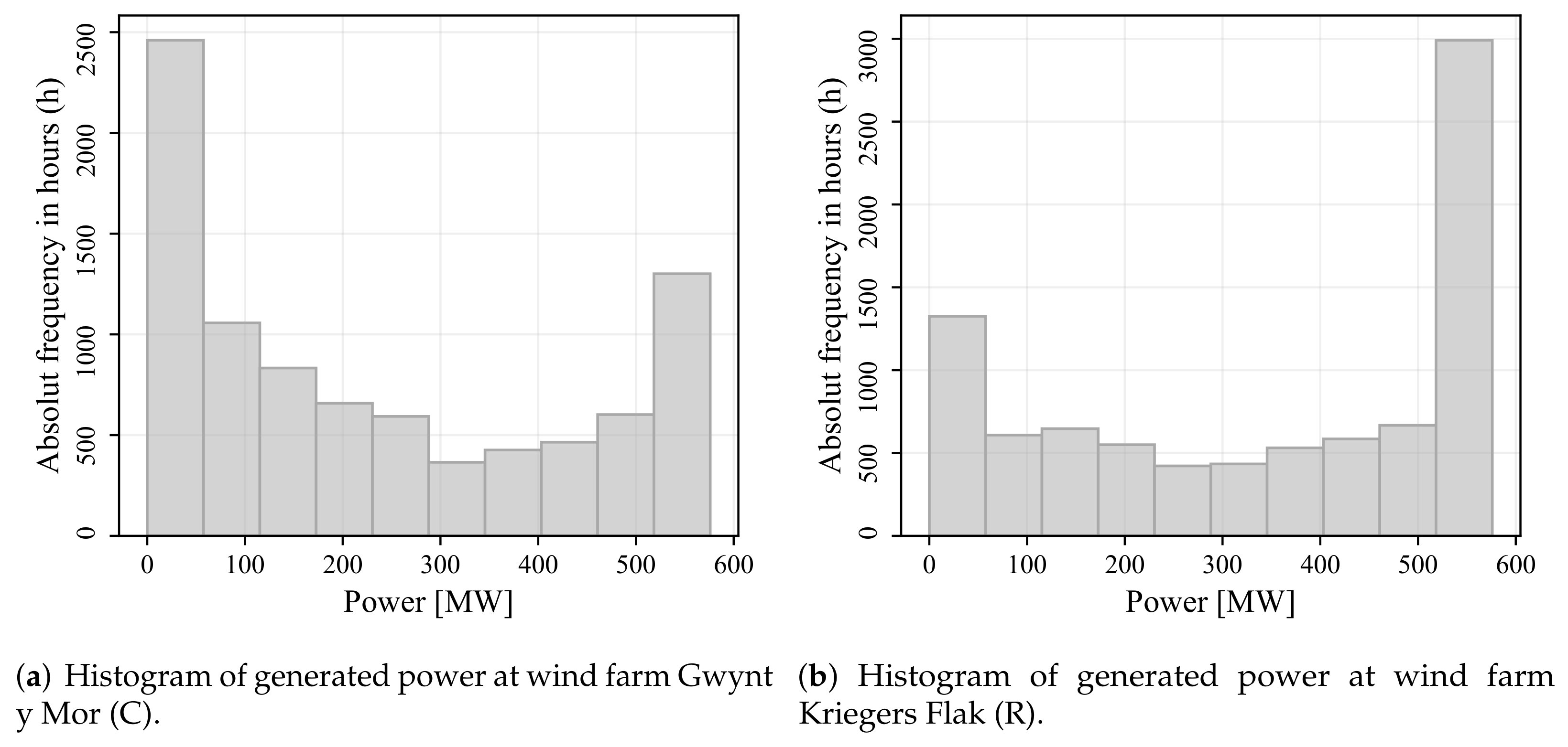
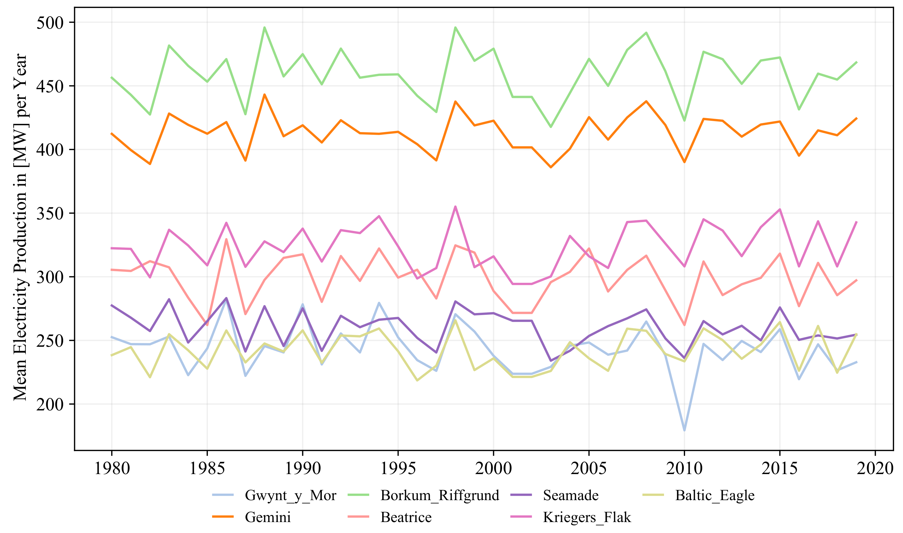
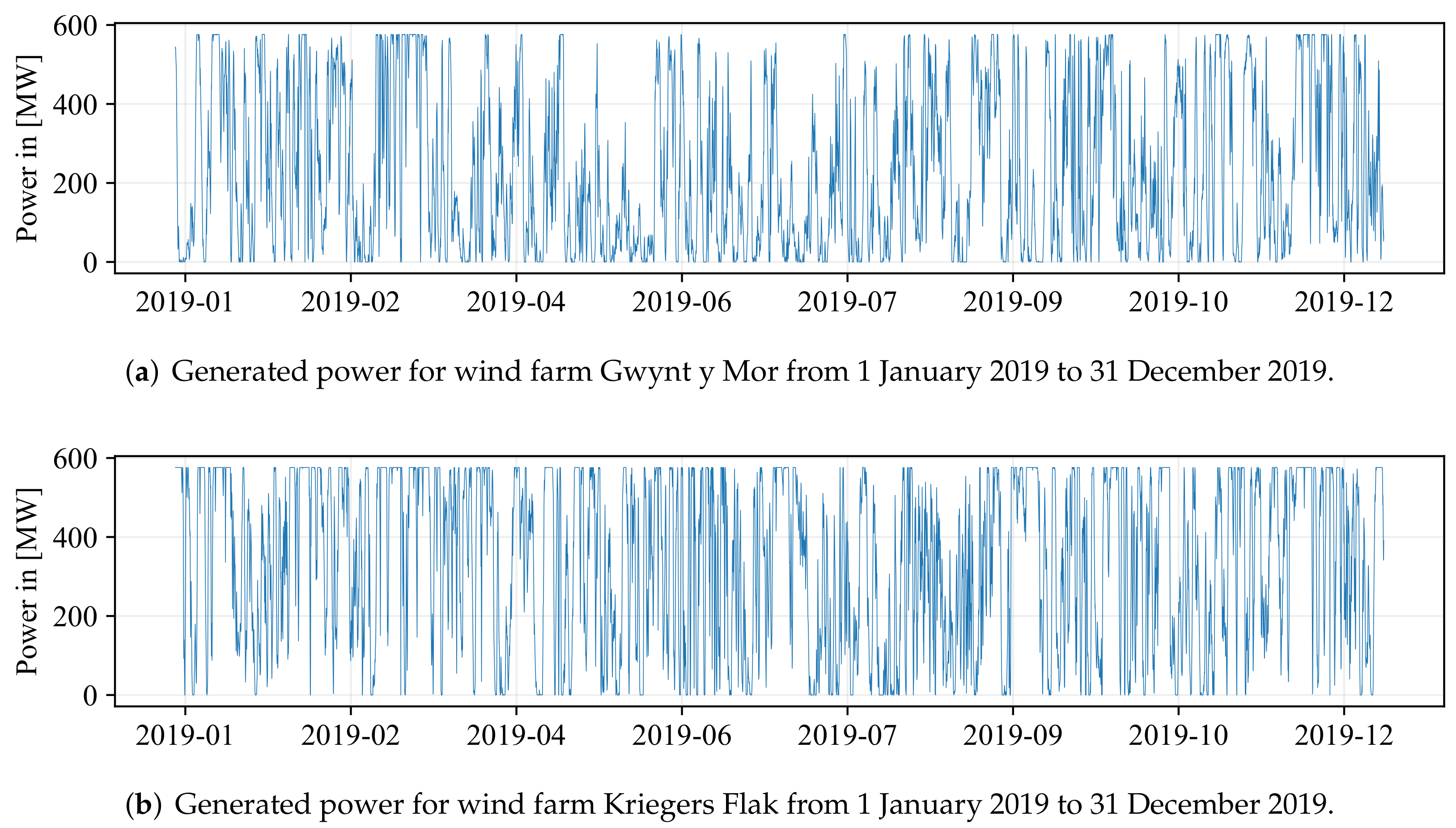
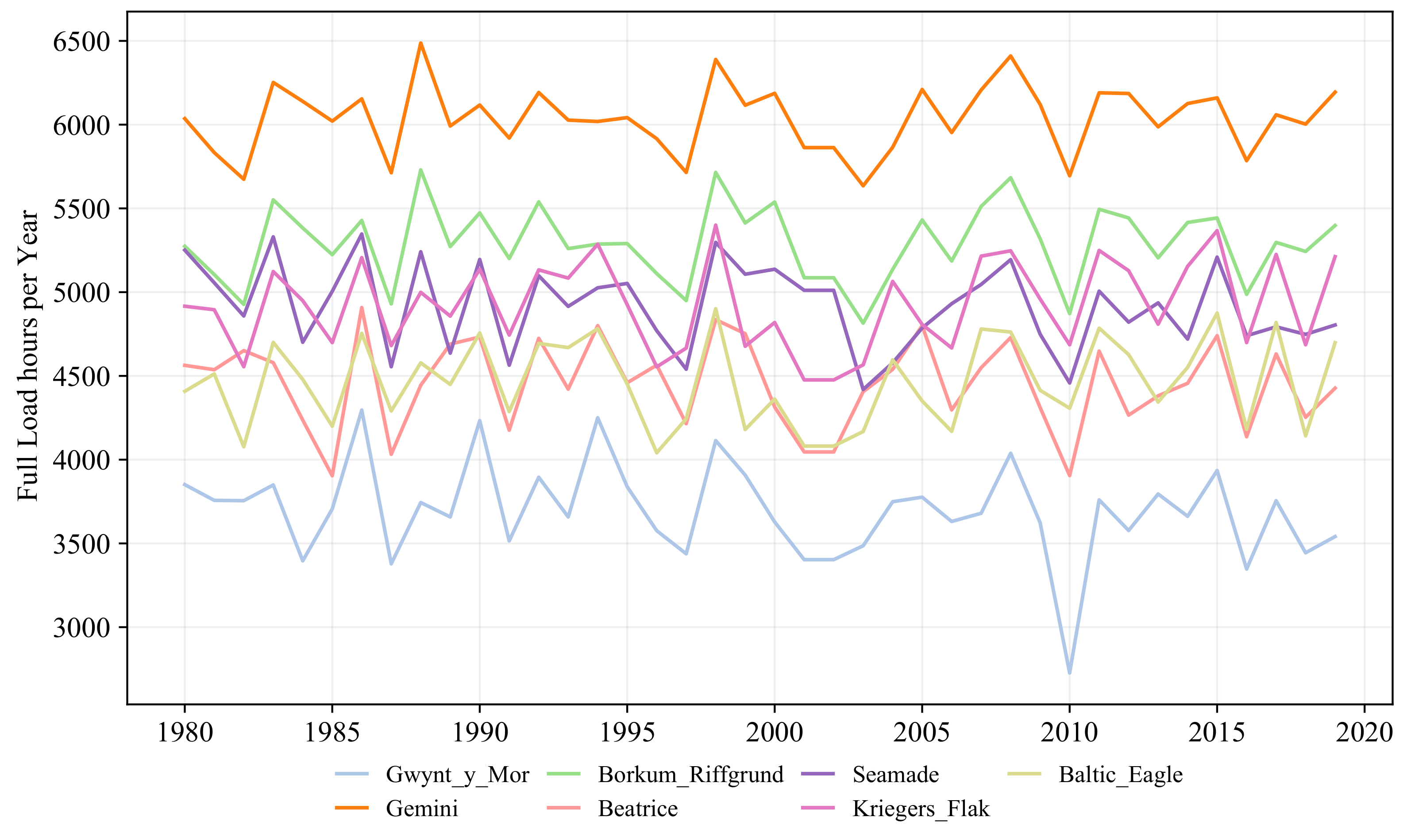
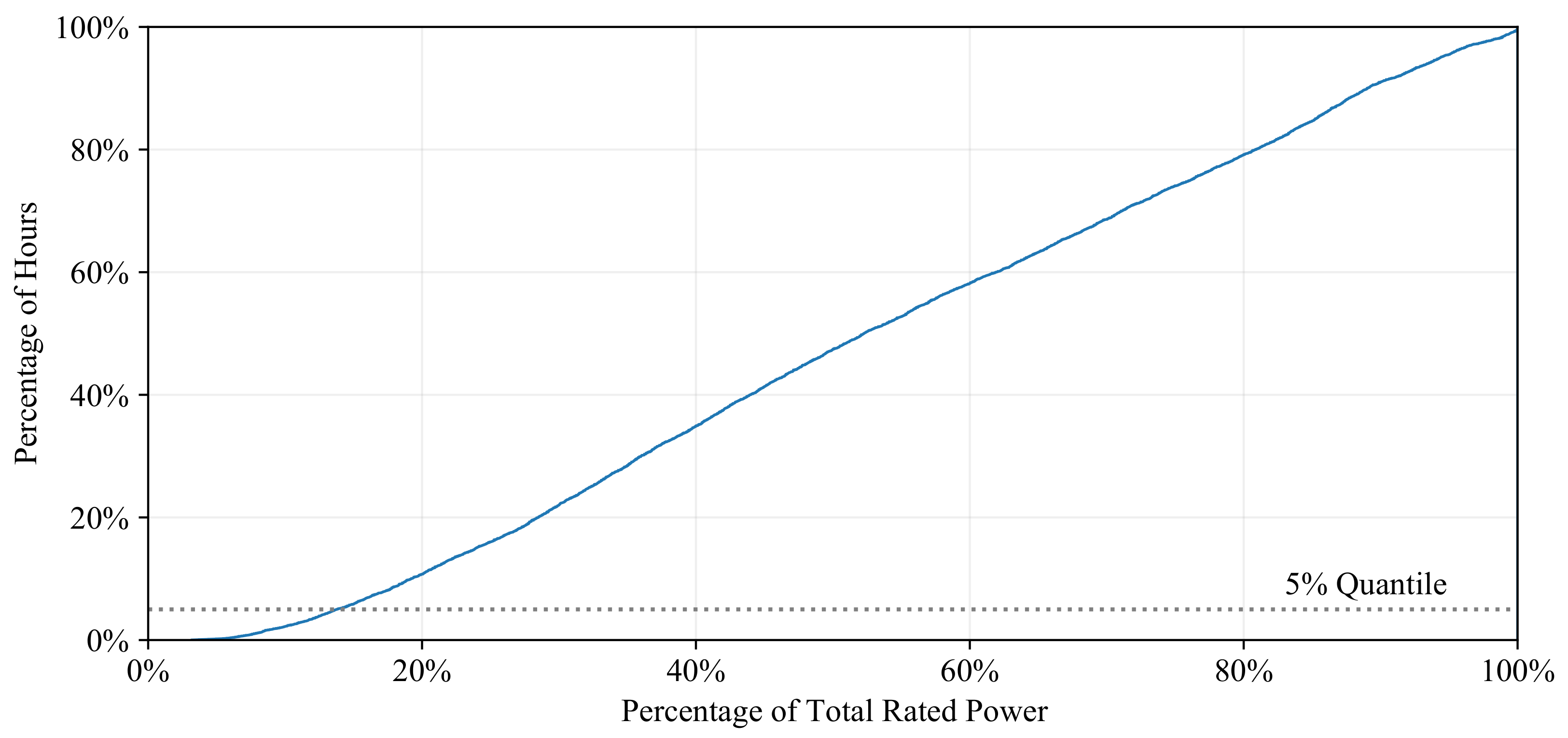
3.1. Descriptive Statistics

In this section, we give results of the descriptive analysis of the data provided. The analysis is intended to give first insights into the data and to enable other scientists to work with the data more quickly. We report quantiles, mean, standard deviations, number of rated power hours (R.-Power), full-load hours (Full-L.), number of cut-out hours (Offs), and number of hours below cut-in (Null) of the year 2019 in Table 2. The same tables for earlier years (1980, 1990, 2000, 2010) are given in Appendix B.1.
In total, the time series of 2019 consists of 8760 data points, i.e., the hours of a non-leap year. Across all wind farms, we observe a relatively small number of cut-out hours where the wind speed was too high for the wind turbines and, thus, turned off. In the other extreme, 506 h on average per wind farm had too light wind conditions to generate electricity. This corresponds to a share of 5.8 % of all hours in 2019. However, on average, each wind farm generates its rated power in 17.6 % of all hours in 2019. In total across all wind farms, this corresponds to 4704 full-load hours. To get a more detailed picture, Figure 6 shows histograms of the hourly output power at Gwynt y Mor (C) and Kriegers Flak (R). The U-shape visualizes the full-load hours on the right tail and the overpowered/underpowered times and low wind hours in the left tail. E.g., we observe more hours in the left tail at the Gwynt y Mor wind farm due to the higher proportion of lower winds observed in Figure 2.
Turning to the full time horizon, Figure 7 displays the full-load hours from 1980 to 2019 for selected wind farms. At closer inspection, we recognize two interesting aspects in the figure. First, the number of full-load hours seems to be stationary over the years for all wind farms. As a result, the order (by full-load hours) of the wind farms does not significantly change over the years; i.e., the the full-load hours of all wind farms develop parallel over time. Second, it seems that the position of the Gemini wind farm is by far the most attractive. However, this is mainly driven by its relatively small wind turbines (SWT 4.0–130), which reach their rated power slightly earlier than other turbines (see, e.g., figures of the power curves in Appendix C). The full figure for all wind farms and figures for mean production and variability (interquartile range) over the same time horizon can be found in Appendix B.2. There, we observe the same co-monotonous movements, whereas the absolute values in the figures seem to be mainly driven by the nominal power of the wind farm.

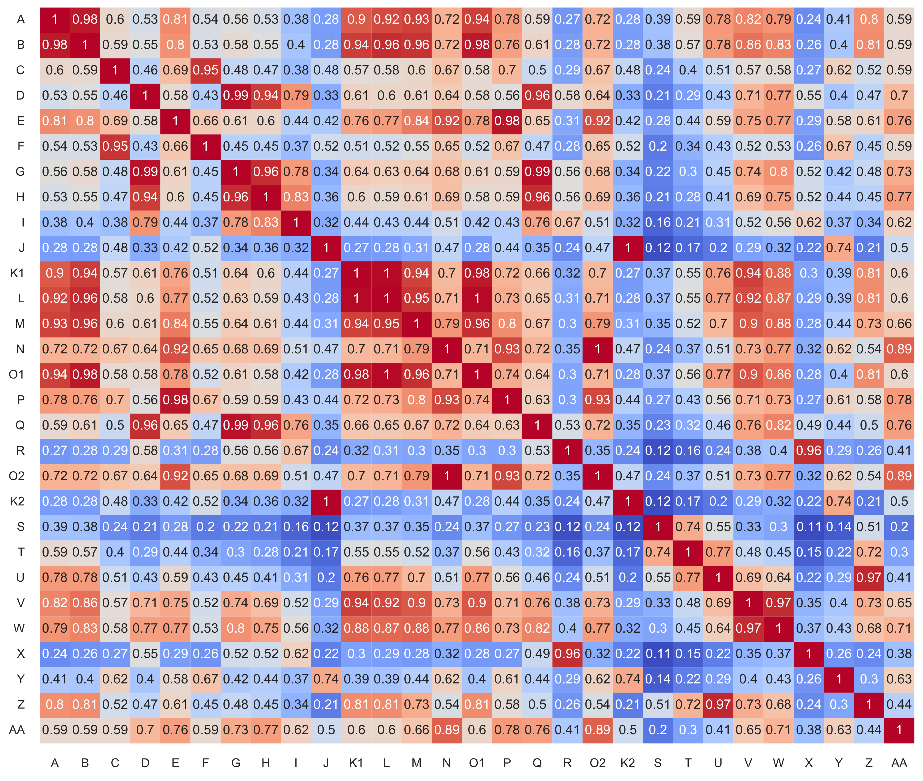
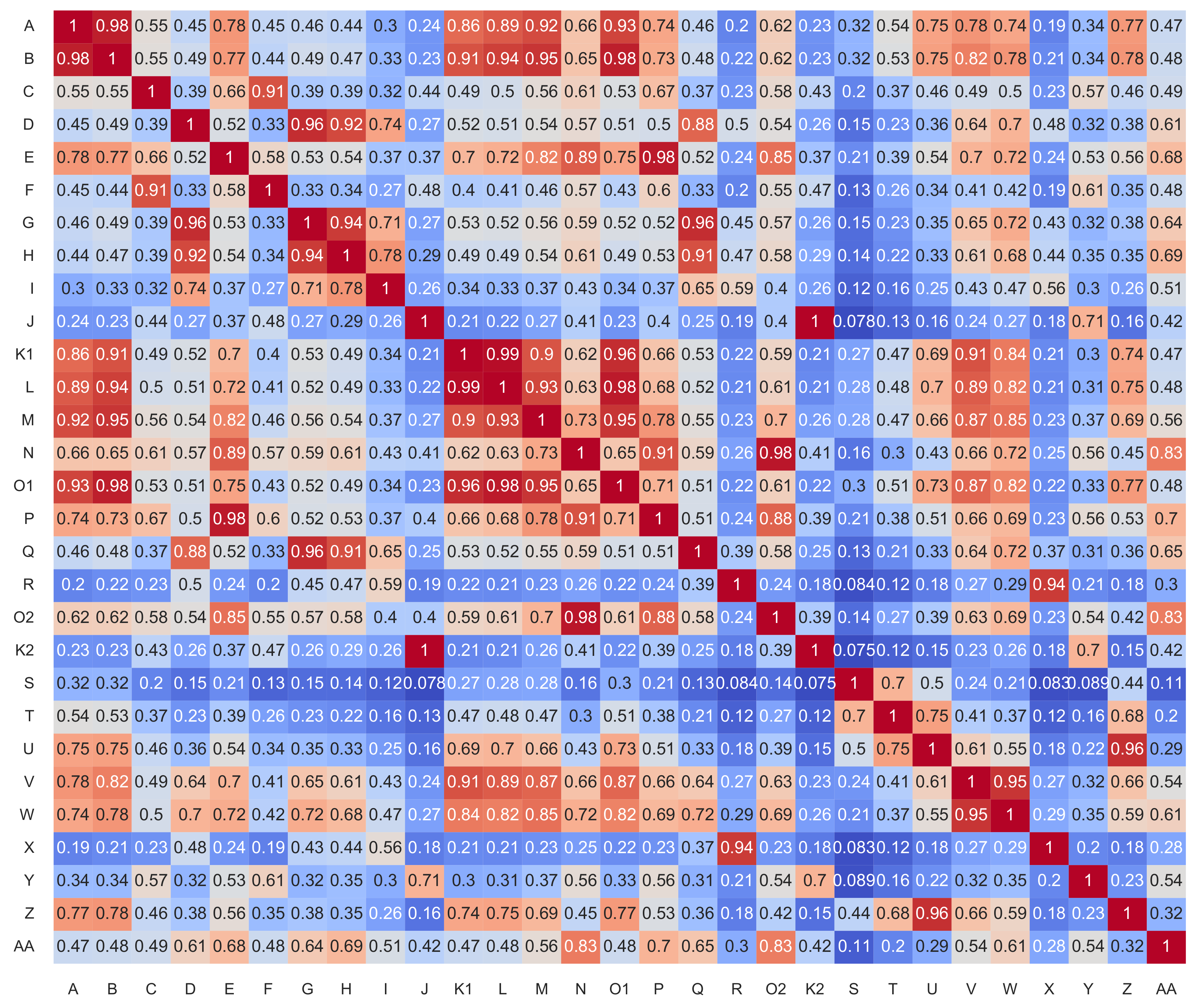
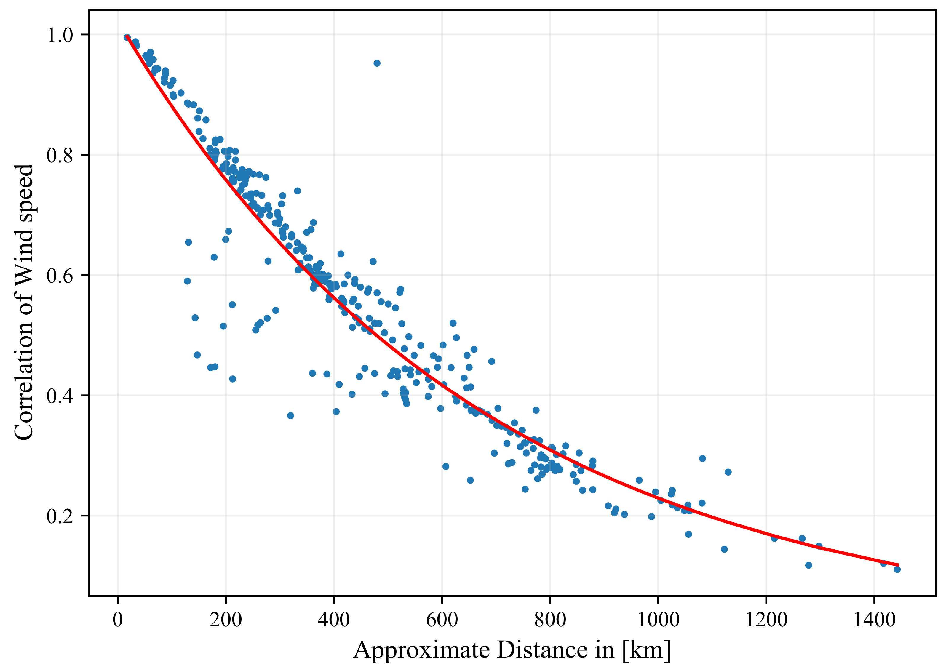
3.2. Dependence Patterns

This section provides an overview of the correlation structure of synthetic power series from different locations. Such dependence analysis is crucial, e.g., for modeling and analyzing uncertainty in the sum of overall produced power and potential balancing effects of geographically more widely distributed installations. For onshore turbines, such effects are investigated, e.g., in [26,32,34,42]. In general, we observe that dependence and joint distributional information across units or time are increasingly considered by researchers contributing to the energy literature, such as, e.g., [43,44,45,46] in the forecasting context.
We study the correlation structure of the data to evaluate the overall potential to reduce the offshore wind power variability by considering wind farms in diverse geographical locations and with diverse technical specifications in Europe. Therefore, we first analyze the correlation between wind speeds at different locations before turning to the correlations of the resulting power output. Looking at both wind speed and power output enables us to disentangle the effect of the turbines’ power curves from the effect of different wind speeds at geographical locations. The correlation matrix of wind speeds is shown in Figure 8.
At first glance, the correlation of wind speed ranges from 0.11 up to values of 1.0 , i.e., perfect correlation. It is notable that all correlations are positive, indicating a similar behavior of wind speeds over all locations, which is driven by synoptic-scale weather effects. Hence, no perfect balancing effects in energy production due to negative correlations in wind speeds can be expected. Moreover, we observe that the wind speed at les dYeu et de Noirmoutir (S) seems to be least dependent on the wind speeds of the other wind farms. This, by far the most southwestern location, is the only one in the Atlantic Ocean. Indeed, a comparison with the distance matrix of the wind farms reveals that the correlation is mainly dependent on the distances between the wind farms (the distance matrix of wind farms is shown in Figure A7). This is also illustrated in Figure 9, which plots pairwise correlations of two sites against their distance. A fitted exponential model ρ e x p ( d i s t a n c e / D ) , results in a decay parameter D = 668.66 km and an intercept of ρ = 1.02 for zero distance. Most interesting, this decay parameter is of similar size as in studies for onshore locations. For example, refs. [32,33,34] found exponential decay parameters of 305, 455, and 723 km, respectively. Here, refs. [32] used data from Texas, while ref. [33] used European data and ref. [34] focused on Germany. Note that these numbers should be compared with care, since the considered frequencies vary from 15 min data over hourly data to data from one 10 min average every 3 h in those studies. However, a characteristic difference we see compared to the onshore studies is that the intercept of the fitted relationship is nearly 1. This has been around 0.9 for the onshore studies. This result seems to be intuitive, since specific surface conditions or obstacles might reduce the correlation between neighbored onshore locations, while this does not hold for offshore locations, at least as long we abstract from the interaction between neighbored turbines.
In the second step of the dependence analysis, we analyze the correlation of derived power signals from each wind farm (see Section 2 for the conversion of wind signals to power signals). The corresponding correlation matrix is shown in Figure 10. Here, a similar but slightly weaker correlation is observed. We explain this by the flattening effect of cut-in speeds and nominal wind speeds in the time series.
To sum up, the lower correlation values of power signals suggest that the geographic diversification and technical details of wind farms lead to a reduced variance in the total energy production, i.e., balancing effects across wind farms and a more stable energy production compared to the power output of a single wind farm. It now seems reasonable to look at the CDF of the total energy generation from all wind farms. This graphical representation of the data enables us to analyze the nature of the total energy generation in Europe, e.g., observing lower bounds of energy production or quantiles. The CDF of the total hourly electricity generation in 2019 is shown in Figure 11. The figure displays the percentage of total rated power versus the percentage of all hours in 2019. We observe that the 1% quantile (5%/10%) of total power generation is 1772.27 MW (3165.34 MW/4415.74 MW), which corresponds to 7.7% (13.7%/19.2%) of the rated power. This means that the considered wind farms generated more than 1.7 GW in 99% of the time and produced more than 13.8% of the total rated power in 95% of the time. Such a high availability of offshore wind energy production is particularly important at night, where other renewable energy sources such as solar power produce less electricity.
In general, the observed results from 2019 seem to indicate no exception over the observed years in our study. In Figure 12, we show the 1%, 5%, and 10% quantile of total power generation from 1980 to 2019. It is interesting to see that these quantiles remain relatively stationary across years with no discernible trend structure or multi-year seasonal variation. Moreover, we find that there are no hours without power generation and only very few hours when the entire system collectively generates the rated power over the years (the annual rated power hours vary around 20 throughout the data). These very few observations of extreme situations in the system prove the overall balancing effect despite observed positive correlations.

4. Conclusions

In this paper, we compile an openly available data set covering 40 years of hourly wind speeds and synthetic historic production signals for the 29 biggest offshore wind farms in Europe. More precisely, the data set contains data from 1980 to 2019 of already operating wind farms as well as such under construction up to 2024. We provide detailed information about the currently installed or planned wind turbine types and give analytical expressions for the power curves. Furthermore, we present a first descriptive analysis of the data and the joint electricity generation of these current offshore wind farms in Europe. We find relative high volatility and intermittency at single locations with balancing potential when interconnecting spatially more distant locations, since dependency patterns between locations prove to weaken with growing distance. We explain in detail how the wind speed data set and production signals were generated based on the ERA5 data set [35], so that researchers making use of our data may easily integrate more current data as soon as available. The same holds for the planned extension of the historical period of the ERA5 data set back to 1950, which would then also open up the possibility of doing very long-term studies as well.

Author Contributions

Conceptualization, O.G., F.K. and M.W.; methodology, O.G., F.K. and M.W.; software, F.K.; validation, O.G., F.K. and M.W.; formal analysis, F.K.; investigation, O.G., F.K. and M.W.; resources, O.G., F.K. and M.W.; data curation, F.K.; writing—original draft preparation, O.G., F.K. and M.W.; writing—review and editing, O.G., F.K. and M.W.; visualization, O.G., F.K. and M.W.; supervision, O.G. All authors have read and agreed to the published version of the manuscript.

Funding

This research received no external funding.

Institutional Review Board Statement

Not applicable.

Informed Consent Statement

Not applicable.

Data Availability Statement

The data presented in this study are openly available through the following doi [https://doi.org/10.6084/m9.figshare.19139648.v1] and generated using Copernicus Climate Change Service information (1980–2019) containing modified Copernicus Climate Change Service information (1980–2019).

Acknowledgments

The work was partly supported by the German Federal Ministry of Economic Affairs and Climate Action through the research project ProKoMo within the Systems Analysis Research Network of the 6th energy research program. Furthermore, we thank Tim Michael Seeberger for programming assistance and acknowledge support by the KIT-Publication Fund of the Karlsruhe Institute of Technology. We also thank three anonymous referees for their insightful comments, which have helped us to improve the paper.

Conflicts of Interest

The authors declare no conflict of interest.

Appendix A. Sources Information on Each Wind Farm

Table A1. Information sources for wind farms.
Wind FarmInformation Source
Ahttps://londonarray.com
Bhttps://sserenewables.com/offshore-wind/operations/greater-gabbard/
Chttps://rwe.com/-/media/archive/ir-archiv/weitere-inhalte/downloads/Download-aspx-pmid-4004961-datei-1.pdf
Dhttps://orsted.de/gruene-energie/offshore-windenergie/unsere-offshore-windparks-nordsee/
Ehttps://orsted.co.uk/energy-solutions/offshore-wind/our-wind-farms
Fhttps://walneyextension.co.uk/about-the-project#project-timeline-2018
Ghttps://orsted.co.uk/energy-solutions/offshore-wind/our-wind-farms
Hhttps://enbw.com/erneuerbare-energien/windenergie/unsere-windparks-auf-see/hohe-see/
Ihttps://powerplants.vattenfall.com/de/horns-rev/
https://orsted.com/en/our-business/offshore-wind/our-offshore-wind-farms
https://powerplants.vattenfall.com/de/horns-rev-3/
Jhttps://www.beatricewind.com
K1https://deme-group.com/news/turbine-installation-borssele-1-2-successfully-completed-deploying-deme-offshores-unique
Lhttps://www.nsenergybusiness.com/projects/seamade-offshore-wind-farm-north-sea/
Mhttps://iberdrola.com/about-us/lines-business/flagship-projects/east-anglia-one-offshore-wind-farm
Nhttps://hornseaprojectone.co.uk
O1https://www.blauwwind.nl/en/
Phttps://tritonknoll.co.uk/about-triton-knoll/
Qhttps://www.geminiwindpark.nl
Rhttps://group.vattenfall.com/de/newsroom/news/2021/offshore-windpark-kriegers-flak-fertiggestellt
O2https://hornseaprojects.co.uk/hornsea-project-two
K2https://morayeast.com/project
Shttps://eoliennesenmer.fr/facades-maritimes-en-france/facade-nord-atlantique-manche-ouest/iles-d-yeu-et-noirmoutier
Thttps://iberdrola.com/about-us/lines-business/flagship-projects/saint-brieuc-offshore-wind-farm
Uhttps://nawindpower.com/construction-commences-on-the-fecamp-offshore-wind-farm
https://parc-eolien-en-mer-de-fecamp.fr/faq/
Vhttps://vattenfall-hollandsekust.nl/en/wind-farm
Whttps://www.crosswindhkn.nl/
Xhttps://iberdrola.com/about-us/lines-business/flagship-projects/baltic-eagle-offshore-wind-farm
Yhttps://seagreenwindenergy.com/
Zhttps://eoliennesenmer.fr/facades-maritimes-en-france/facade-manche-mer-du-nord/dieppe-le-treport
AAhttps://doggerbank.com

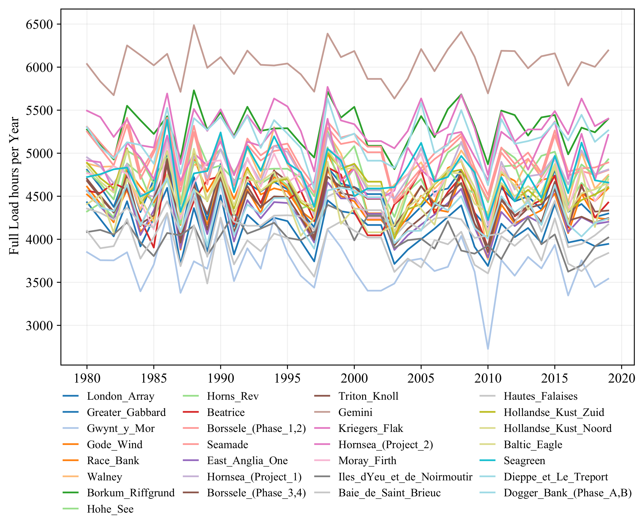
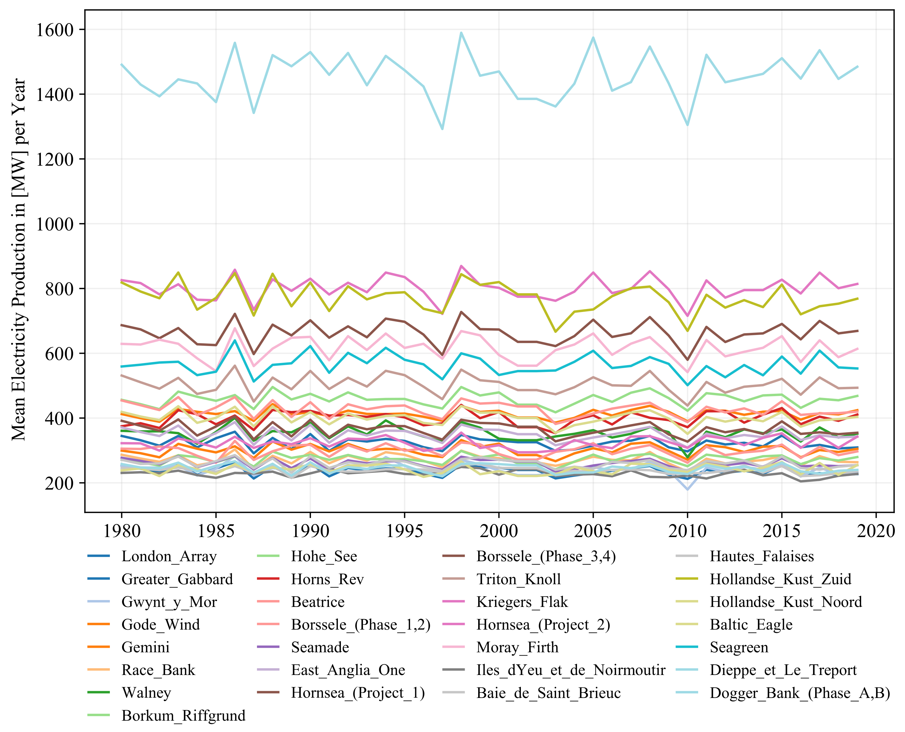
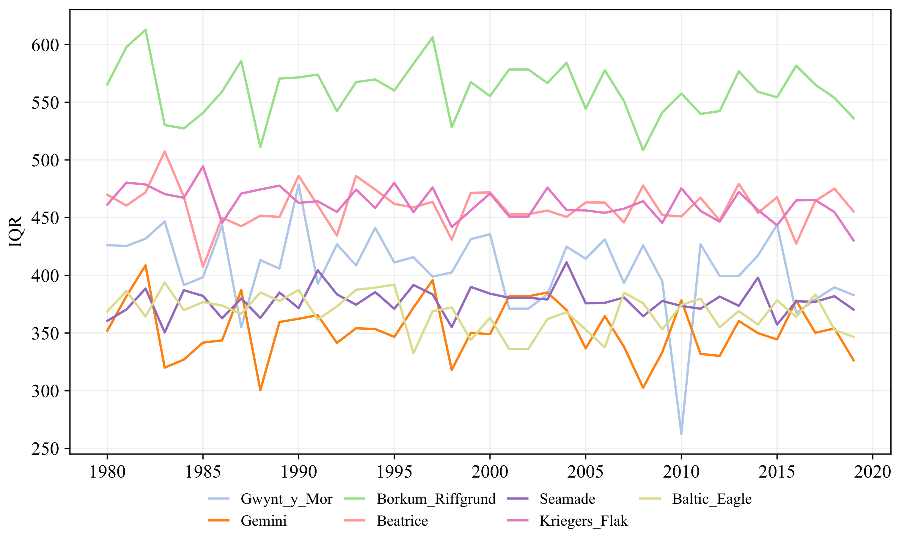
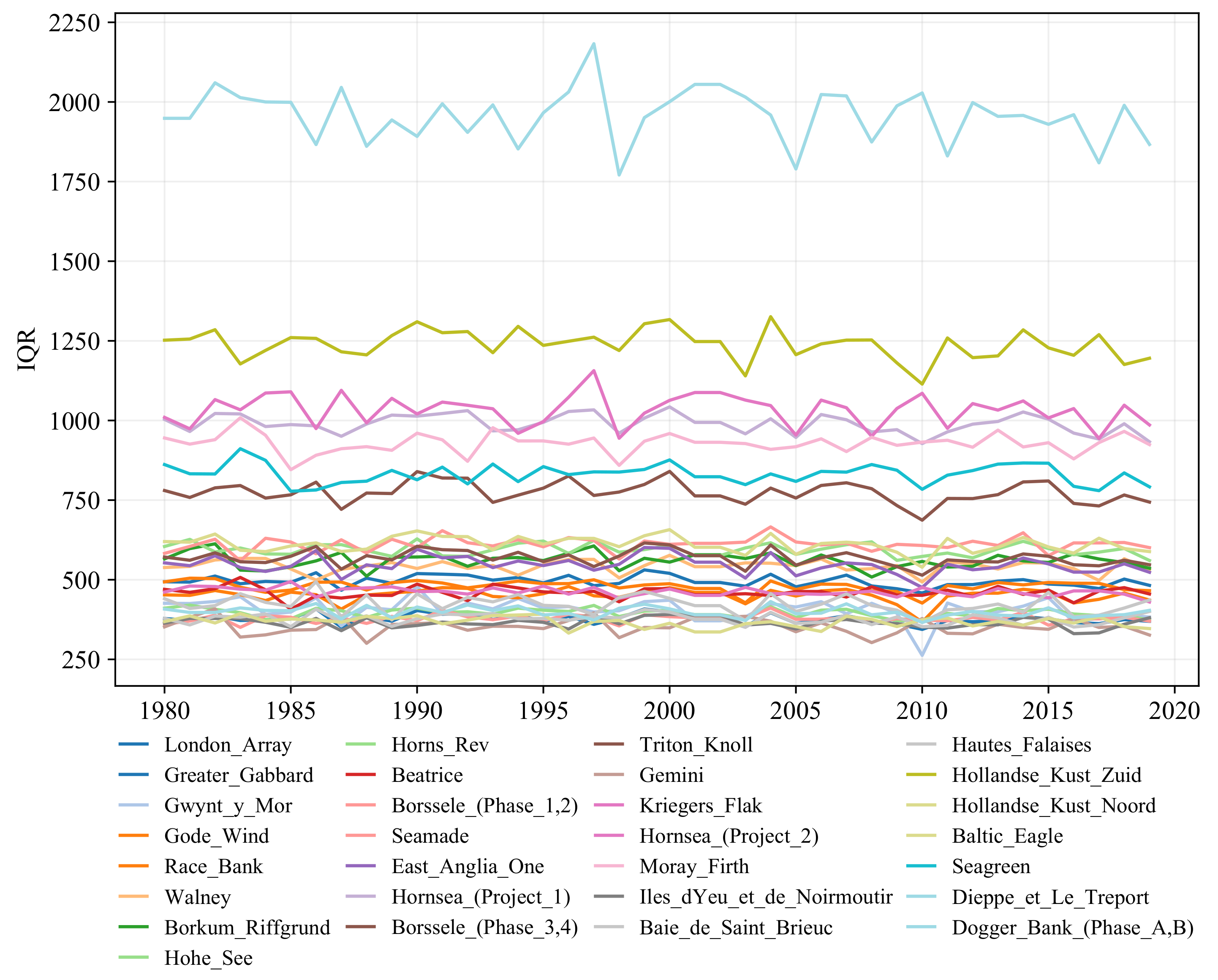
Appendix B. Descriptive Statistics for Various Time Horizons

Appendix B.1. Tables

Table A2. Descriptive statistics of synthetic power production at the wind farms for the year 1980.
Mean0.25-Q0.5-Q0.75-QSDR.-PowerFull-L.OffsNull
A344.79112.90352.29606.51236.14174148070519
B254.2072.57234.46450.94185.5791644300484
C252.5448.99201.47475.16211.0362138510636
D299.5983.37263.12576.73223.25207345210462
E412.30248.01493.28600.00204.32306560363182
F286.7186.33256.74538.89208.22195046120516
G360.69104.29377.10642.68250.81185348811527
H456.37194.59493.10760.00279.67236952740220
I270.9578.79274.75489.47190.09197147882492
J374.6992.72335.09697.14287.3192743231632
K1305.4881.07298.45550.93222.47155745630595
L454.37169.26533.23752.00285.74230453071470
M277.42103.44319.37464.00175.70221852511484
N371.11115.21358.96668.18264.69154745652482
O1686.70210.98710.801214.39464.26208549520466
P391.59126.07386.09697.35271.91166247021459
Q531.29163.14522.94943.24373.00153146780495
R322.41107.55343.74568.82218.31195049163611
O2825.74310.27997.411320.00503.90270854941439
K2629.07179.07644.881124.15441.91176147670558
S230.6453.46198.06417.05182.44117640840699
T246.0563.29232.37441.86185.09129543572543
U271.1462.38227.58502.86216.39116340990630
V857.17273.62897.531525.67584.28199448894460
W419.06129.04431.50748.93287.49193848492452
X238.4166.44219.24435.08177.01149344085576
Y559.23146.60579.131008.16399.38172847233703
Z258.0563.18249.20471.11191.12164245691648
AA1490.85521.421745.252470.00950.972551530123411
Total12,678.627247.0112,416.4018,591.276369.4851,78948475614,851
Table A3. Descriptive statistics of synthetic power production at the wind farms for the year 1990.
Mean0.25-Q0.5-Q0.75-QSDR.-PowerFull-L.OffsNull
A344.79112.90352.29606.51236.14174148070519
B254.2072.57234.46450.94185.5791644300484
C252.5448.99201.47475.16211.0362138510636
D299.5983.37263.12576.73223.25207345210462
E412.30248.01493.28600.00204.32306560363182
F286.7186.33256.74538.89208.22195046120516
G360.69104.29377.10642.68250.81185348811527
H456.37194.59493.10760.00279.67236952740220
I270.9578.79274.75489.47190.09197147882492
J374.6992.72335.09697.14287.3192743231632
K1305.4881.07298.45550.93222.47155745630595
L454.37169.26533.23752.00285.74230453071470
M277.42103.44319.37464.00175.70221852511484
N371.11115.21358.96668.18264.69154745652482
O1686.70210.98710.801214.39464.26208549520466
P391.59126.07386.09697.35271.91166247021459
Q531.29163.14522.94943.24373.00153146780495
R322.41107.55343.74568.82218.31195049163611
O2825.74310.27997.411320.00503.90270854941439
K2629.07179.07644.881124.15441.91176147670558
S230.6453.46198.06417.05182.44117640840699
T246.0563.29232.37441.86185.09129543572543
U271.1462.38227.58502.86216.39116340990630
V857.17273.62897.531525.67584.28199448894460
W419.06129.04431.50748.93287.49193848492452
X238.4166.44219.24435.08177.01149344085576
Y559.23146.60579.131008.16399.38172847233703
Z258.0563.18249.20471.11191.12164245691648
AA1490.85521.421745.252470.00950.972551530123411
Total12,678.627247.0112,416.4018,591.276369.4851,78948475614,851
Table A4. Descriptive statistics of synthetic power production at the wind farms for the year 2000.
Mean0.25-Q0.5-Q0.75-QSDR.-PowerFull-L.OffsNull
A330.4385.73319.67605.82243.07174546075742
B246.7854.30223.85453.10191.02901430011763
C237.9131.05164.75466.70216.3967036281934
D321.1194.44311.38582.00225.96227448466476
E422.61250.99534.79600.00206.433453618721223
F276.1065.28238.59540.44214.37203344419683
G336.3564.53313.06641.23261.05192645522858
H479.19204.63566.49760.00282.16266055389235
I287.5993.78316.70497.00190.722224508223466
J418.59124.96435.82733.31289.591211482930505
K1288.8263.43264.44535.30224.38152743147758
L447.32140.77535.38752.00296.012413522513660
M271.3779.86317.56464.00182.592303513717713
N363.6681.04343.69679.65276.491647447314752
O1673.38175.35686.301218.00481.722278485612608
P383.4196.02377.91705.43281.271660460415723
Q511.52119.41484.42959.55385.91173945047616
R316.0588.89338.61559.78220.601774481914564
O2802.01256.79969.981320.00523.912840533713586
K2594.70140.48572.581099.54446.351723450710720
S225.2140.28179.59431.37189.01129639885796
T246.1853.64231.42451.99189.14136743591702
U271.1458.01237.82499.41216.43123040993722
V855.14218.80904.521535.63602.402082487728577
W417.46100.27442.30757.59298.642116483124608
X235.9059.80229.77423.12176.581283436214610
Y532.94122.23511.90998.37402.55177045015662
Z257.7861.86257.75470.46190.55163045654755
AA1470.09469.181701.902470.00969.332730522846487
Total12,520.726594.4012,598.4318,722.446597.8954,505478636918,504
Table A5. Descriptive statistics of synthetic power production at the wind farms for the year 2010.
Mean0.25-Q0.5-Q0.75-QSDR.-PowerFull-L.OffsNull
A297.1677.74255.68536.33229.23103341310732
B212.3543.45170.07387.56177.5442636900743
C179.3625.02106.46287.69186.0329627271949
D271.4776.05221.49502.82213.37145140863616
E390.13221.71436.01600.00204.112312569511217
F234.9554.89177.55422.18198.55123737693637
G278.9750.50211.46543.57242.27966376514837
H422.74169.20418.22726.73273.73170248726250
I251.3973.50239.53446.43182.78139544314520
J371.7589.82350.85663.05279.6452542770614
K1262.1244.47212.56495.58221.59123939051889
L387.6295.81375.97703.41287.56148945151684
M236.1356.44224.64429.94176.83142044580692
N308.7570.03250.92545.66254.1389237882671
O1579.98138.60500.781066.14453.45135841718544
P327.2573.12274.23587.32264.0794439180669
Q438.5698.34354.71785.40359.2197938510564
R308.1580.08322.51555.51222.81169446860745
O2715.67200.20739.361285.54507.17186447499519
K2541.8499.30463.711031.34442.61141040953836
S222.4350.26185.14401.77179.7699239285621
T228.9657.56194.90410.06179.9795040430609
U239.0853.91186.55419.59202.6073136040697
V709.00178.53593.401292.82564.10119740339592
W351.2088.85298.82628.08277.06120040538545
X233.5552.78217.79427.16179.11129943070733
Y501.54120.08457.87904.03385.89123842240748
Z226.9346.91192.11412.96182.42101740070759
AA1304.99380.171239.562408.34938.001868462812444
Total11,034.016089.9210,368.2415,676.435770.3435,124420610018,676

Appendix B.2. Figures

Figure A1. Full-load hours of all wind farms from 1980 to 2019. Every line illustrates the yearly full-load hours of one wind farm.
Energies 15 01700 g0a1
Figure A2. Mean production of selected wind farms from 1980 to 2019. Every line illustrates the yearly mean production of one wind farm.
Energies 15 01700 g0a2
Figure A3. Mean production of all wind farms from 1980 to 2019. Every line illustrates the mean production of one wind farm.
Energies 15 01700 g0a3
Figure A4. Interquartile range of selected wind farms from 1980 to 2019. Every line illustrates the yearly interquartile range (IQR) of one wind farm.
Energies 15 01700 g0a4
Figure A5. Interquartile range of all wind farms from 1980 to 2019. Every line illustrates the yearly interquartile range (IQR) of one wind farm.
Energies 15 01700 g0a5

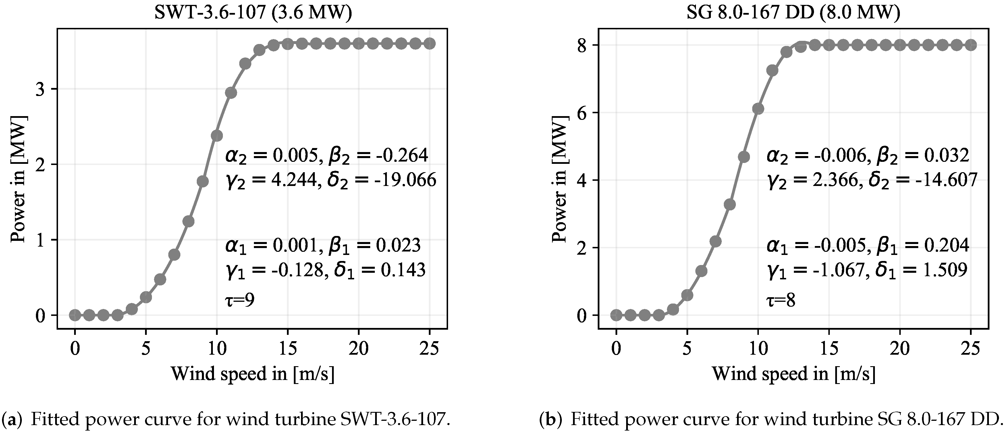
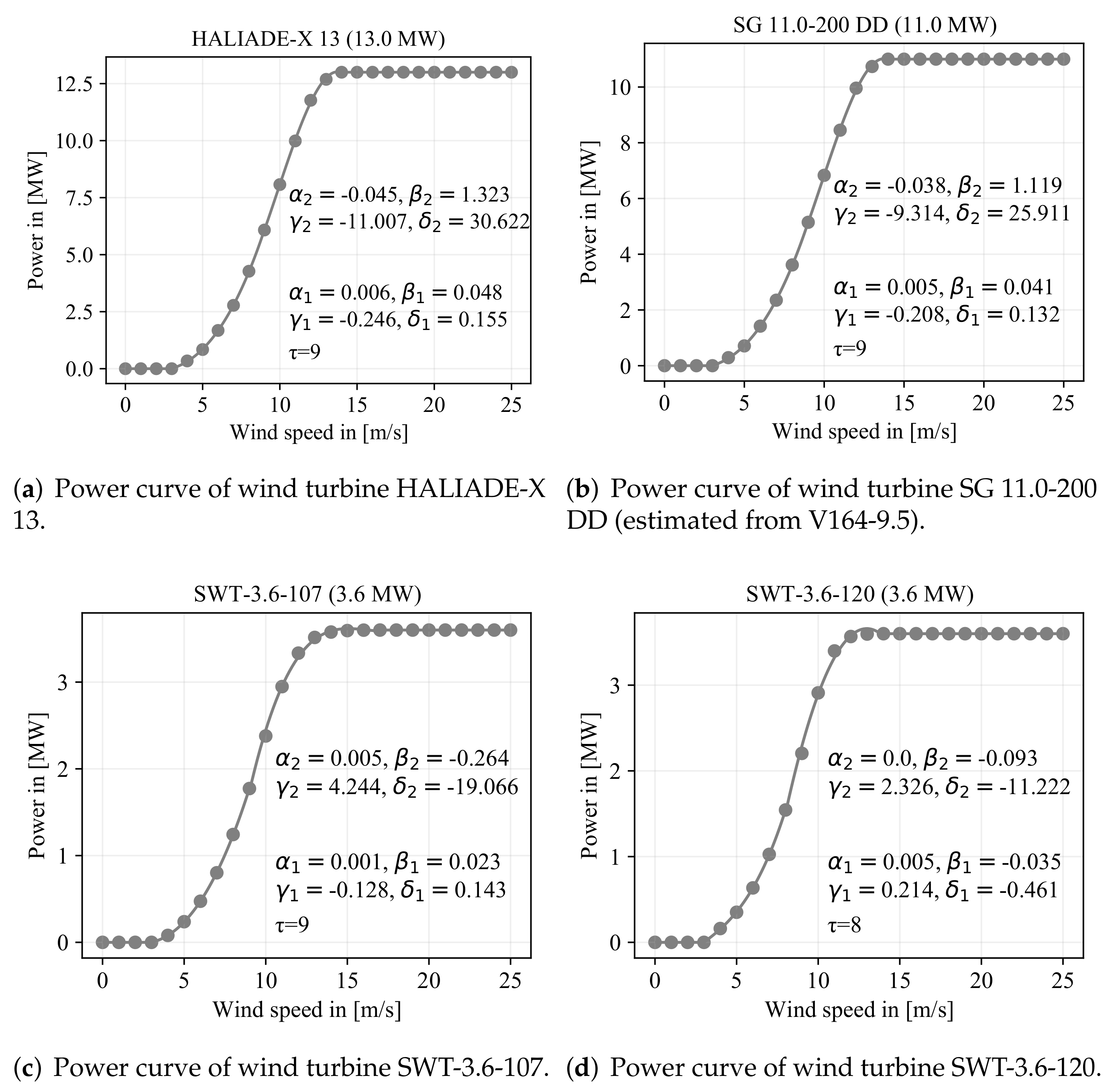
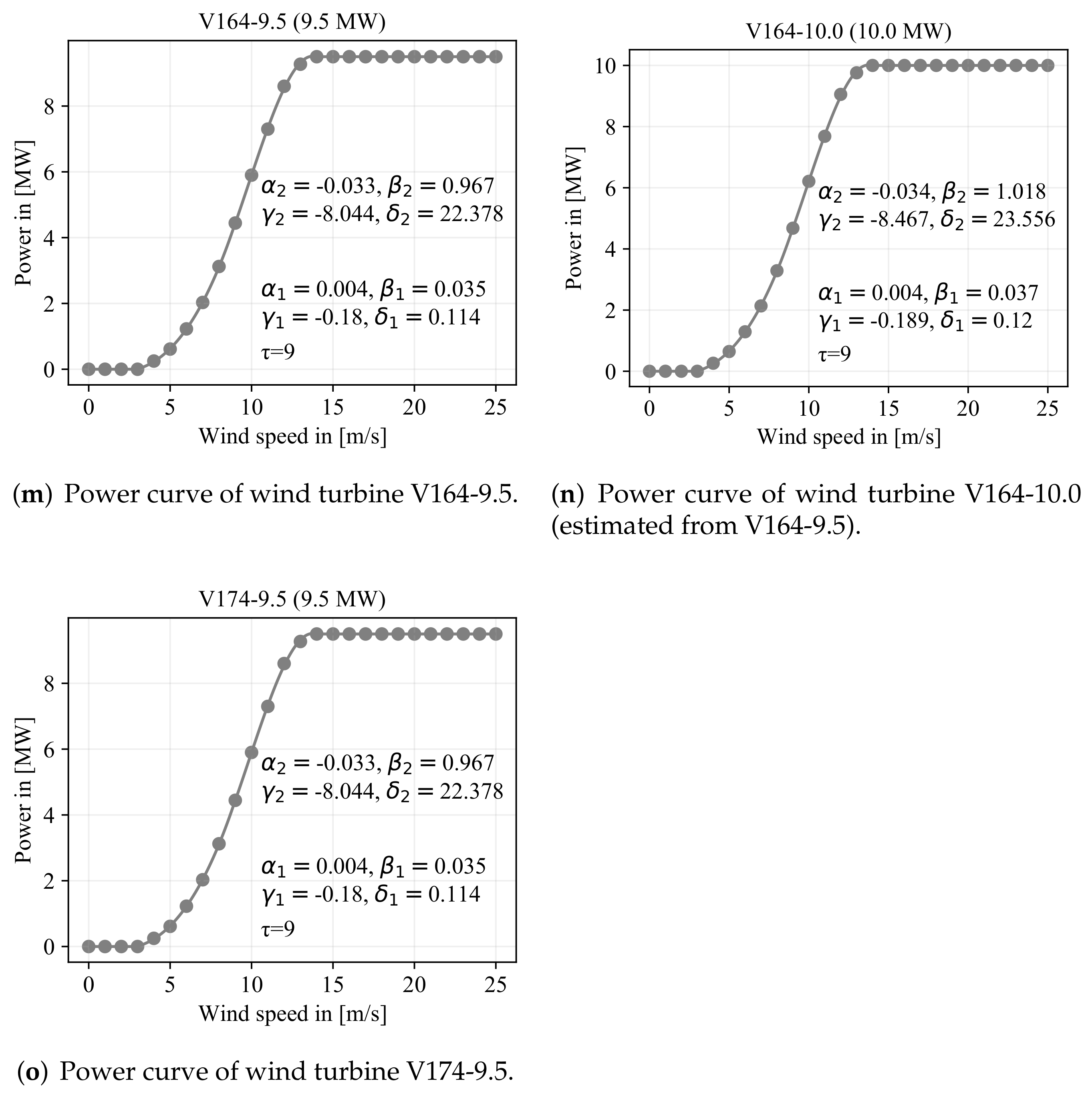
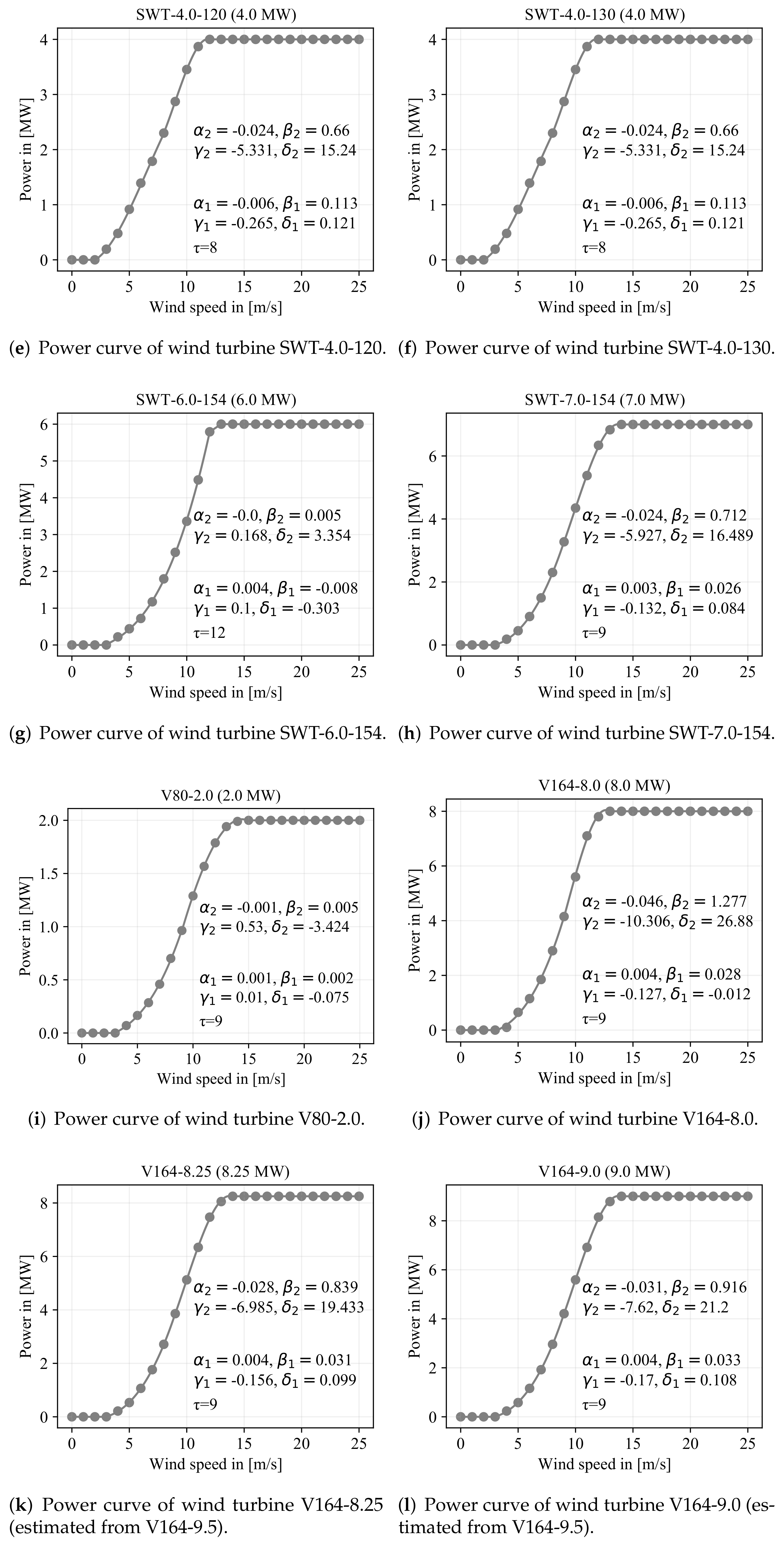
Appendix C. Power Curves of Wind Turbines

Figure A6. Power curves of wind turbines used in the study.
Energies 15 01700 g0a6aEnergies 15 01700 g0a6bEnergies 15 01700 g0a6c

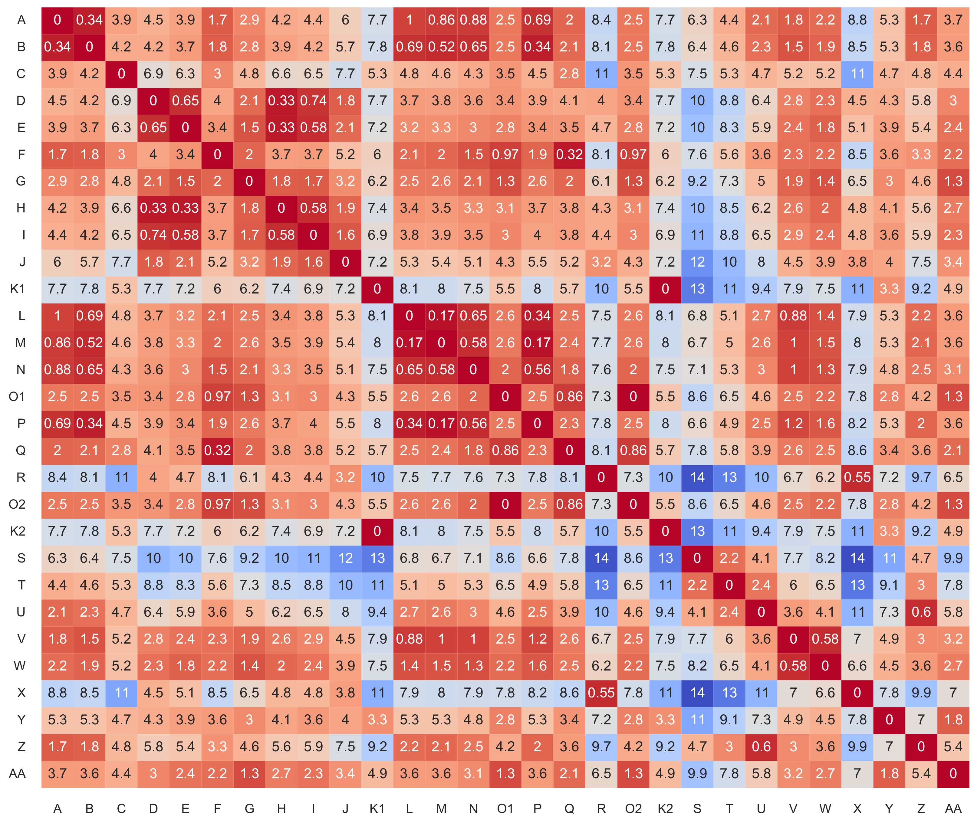
Appendix D. Distance Matrix of Wind Farms

We calculated the distance based on their positions assuming that the Earth is a sphere. Thus, we model the Earth with a radius of r = 6370 km and calculated the distance d ( A , B ) of two points A and B by
d ( A , B ) = r * a r c c o s ( s i n [ l a t i t u d e ( A ) ] * s i n [ l a t i t u d e ( B ) ] + c o s [ l a t i t u d e ( A ) ] * c o s [ l a t i t u d e ( B ) ] * c o s [ l o n g i t u d e ( B ) l o n g i t u d e ( A ) ] )
with angles expressed in radians.
Figure A7. Distance matrix of wind speed of considered wind farms. Shown are pairwise distances in 100 km, each calculated from the two positions from the respective sites in the ERA5 grid. For clearer representation, the matrix elements are colored from dark red (same position) to dark blue.
Energies 15 01700 g0a7

References

  1. EU. Communication from the Commission to the European Parliament, the Council, the European Economic and Social Committee and the Committee of the Regions an EU Strategy to Harness the Potential of Offshore Renewable Energy for a Climate Neutral Future. Available online: https://ec.europa.eu/energy/topics/renewable-energy/eu-strategy-offshore-renewable-energy_en (accessed on 23 December 2021).
  2. EU. Communication from the Commission to the European Parliament, the Council, the European Economic and Social Committee and the Committee of the Regions the European Green Deal. Available online: https://eur-lex.europa.eu/legal-content/EN/TXT/?qid=1576150542719&uri=COM%3A2019%3A640%3AFIN (accessed on 29 December 2021).
  3. IEA. World Energy Outlook 2021. Available online: https://www.iea.org/reports/world-energy-outlook-2021 (accessed on 29 December 2021).
  4. European Commission; Joint Research Center (JRC). Enspreso—Wind—Onshore and Offshore. Available online: http://data.europa.eu/89h/6d0774ec-4fe5-4ca3-8564-626f4927744e (accessed on 29 December 2021).
  5. European Commission; Joint Research Centre; Tarvydas, D.; Politis, S.; Volker, P.; Medarac, H.; Dalla Longa, F.; Badger, J.; Kober, T.; Nijs, W.; et al. Wind Potentials for EU and Neighbouring Countries: Input Datasets for the JRC-EU-TIMES Model; Publications Office: Luxembourg, 2018. [Google Scholar]
  6. Hirth, L. The market value of variable renewables. The effect of solar wind power variability on their relative price. Energy Econ. 2013, 38, 218–236. [Google Scholar] [CrossRef] [Green Version]
  7. Jansen, M.F.; Staffell, I.; Kitzing, L.; Quoilin, S.; Wiggelinkhuizen, E.J.; Bulder, B.; Riepin, I.; Müsgens, F. Offshore wind competitiveness in mature markets without subsidy. Nat. Energy 2020, 5, 614–622. [Google Scholar] [CrossRef]
  8. Kitzing, L.; Juul, N.; Drud, M.; Boomsma, T.K. A real options approach to analyse wind energy investments under different support schemes. Appl. Energy 2017, 188, 83–96. [Google Scholar] [CrossRef]
  9. Hirth, L.; Radebach, A. The Market Value of Wind and Solar Power: An Analytical Approach. SSRN Electron. J. 2018, 38, 218–236. [Google Scholar] [CrossRef]
  10. Beiter, P.; Cooperman, A.; Lantz, E.; Stehly, T.; Shields, M.; Wiser, R.; Telsnig, T.; Kitzing, L.; Berkhout, V.; Kikuchi, Y. Wind power costs driven by innovation and experience with further reductions on the horizon. Wiley Interdiscip. Rev. Energy Environ. 2021, 10, e398. [Google Scholar] [CrossRef]
  11. Weigt, H.; von Hirschhausen, C. Price formation and market power in the German wholesale electricity market in 2006. Energy Policy 2008, 36, 4227–4234. [Google Scholar] [CrossRef] [Green Version]
  12. Möst, D.; Genoese, M. Market power in the German wholesale electricity market. J. Energy Mark. 2009, 2, 47–74. [Google Scholar] [CrossRef]
  13. Keles, D.; Genoese, M.; Möst, D.; Ortlieb, S.; Fichtner, W. A combined modeling approach for wind power feed-in and electricity spot prices. Energy Policy 2013, 59, 213–225. [Google Scholar] [CrossRef]
  14. Gil, H.A.; Gomez-Quiles, C.; Riquelme, J. Large-scale wind power integration and wholesale electricity trading benefits: Estimation via an ex post approach. Energy Policy 2012, 41, 849–859. [Google Scholar] [CrossRef]
  15. Paraschiv, F.; Erni, D.; Pietsch, R. The impact of renewable energies on EEX day-ahead electricity prices. Energy Policy 2014, 73, 196–210. [Google Scholar] [CrossRef] [Green Version]
  16. Pape, C.; Hagemann, S.; Weber, C. Are fundamentals enough? Explaining price variations in the German day-ahead and intraday power market. Energy Econ. 2016, 54, 376–387. [Google Scholar] [CrossRef] [Green Version]
  17. Antweiler, W.; Muesgens, F. On the long-term merit order effect of renewable energies. Energy Econ. 2021, 99, 105275. [Google Scholar] [CrossRef]
  18. Beran, P.; Pape, C.; Weber, C. Modelling German electricity wholesale spot prices with a parsimonious fundamental model—Validation & application. Util. Policy 2019, 58, 27–39. [Google Scholar]
  19. Gea-Bermudez, J.; Kitzing, L.; Matti, K.; Kaushik, D.; León, J.P.M.; Sørensen, P. The Influence of Large-Scale Wind Farm Wake Losses and Sector Coupling on the Development of Offshore Grids. SSRN Electron. J. 2021; Preprint. [Google Scholar] [CrossRef]
  20. Wang, N.; Zhou, K.P.; Wang, K.; Feng, T.; Zhang, Y.H.; Song, C.H. Climate Change Characteristics of Coastal Wind Energy Resources in Zhejiang Province Based on ERA-Interim Data. Front. Phys. 2021, 9, 696. [Google Scholar] [CrossRef]
  21. Pryor, S.C.; Barthelmie, R.J. Climate change impacts on wind energy: A review. Renew. Sustain. Energy Rev. 2010, 14, 430–437. [Google Scholar] [CrossRef]
  22. Gernaat, D.E.; de Boer, H.S.; Daioglou, V.; Yalew, S.G.; Müller, C.; van Vuuren, D.P. Climate change impacts on renewable energy supply. Nat. Clim. Chang. 2021, 11, 119–125. [Google Scholar] [CrossRef]
  23. Koivisto, M.; Jónsdóttir, G.M.; Sørensen, P.; Plakas, K.; Cutululis, N. Combination of meteorological reanalysis data and stochastic simulation for modelling wind generation variability. Renew. Energy 2020, 159, 991–999. [Google Scholar] [CrossRef]
  24. Ruiz, P.; Nijs, W.; Tarvydas, D.; Sgobbi, A.; Zucker, A.; Pilli, R.; Jonsson, R.; Camia, A.; Thiel, C.; Hoyer-Klick, C.; et al. ENSPRESO—An open, EU-28 wide, transparent and coherent database of wind, solar and biomass energy potentials. Energy Strategy Rev. 2019, 26, 100379. [Google Scholar] [CrossRef]
  25. Olauson, J.; Bergkvist, M. Modelling the Swedish wind power production using MERRA reanalysis data. Renew. Energy 2015, 76, 717–725. [Google Scholar] [CrossRef]
  26. Koivisto, M.; Ekström, J.; Seppänen, J.; Mellin, I.; Millar, J.; Haarla, L. A statistical model for comparing future wind power scenarios with varying geographical distribution of installed generation capacity. Wind Energy 2016, 19, 665–679. [Google Scholar] [CrossRef]
  27. Jensen, T.V.; Pinson, P. RE-Europe, a large-scale dataset for modeling a highly renewable European electricity system. Sci. Data 2017, 4, 170175. [Google Scholar] [CrossRef] [Green Version]
  28. Andresen, G.B.; Rodriguez, R.A.; Becker, S.; Greiner, M. The potential for arbitrage of wind and solar surplus power in Denmark. Energy 2014, 76, 49–58. [Google Scholar] [CrossRef]
  29. Gupta, R.; Shankar, H. Global Energy Observatory. Available online: http://www.globalenergyobservatory.com/index.php (accessed on 12 January 2021).
  30. Wiese, F.; Schlecht, I.; Bunke, W.D.; Gerbaulet, C.; Hirth, L.; Jahn, M.; Kunz, F.; Lorenz, C.; Mühlenpfordt, J.; Reimann, J.; et al. Open Power System Data—Frictionless data for electricity system modelling. Appl. Energy 2019, 236, 401–409. [Google Scholar] [CrossRef] [Green Version]
  31. Engelhorn, T.; Müsgens, F. How to estimate wind-turbine infeed with incomplete stock data: A general framework with an application to turbine-specific market values in Germany. Energy Econ. 2018, 72, 542–557. [Google Scholar]
  32. Katzenstein, W.; Fertig, E.; Apt, J. The variability of interconnected wind plants. Energy Policy 2010, 38, 4400–4410. [Google Scholar] [CrossRef]
  33. Giebel, G. On the Benefits of Distributed Generation of Wind Energy in Europe. Masters’s Thesis, Carl von Ossietzky Universitat Oldenburg, Oldenburg, Germany, 2000. [Google Scholar]
  34. Grothe, O.; Schnieders, J. Spatial dependence in wind and optimal wind power allocation: A copula-based analysis. Energy Policy 2011, 39, 4742–4754. [Google Scholar] [CrossRef] [Green Version]
  35. Hersbach, H.; Bell, B.; Berrisford, P.; Biavati, G.; Horányi, A.; Sabater, J.M.; Nicolas, J.; Peubey, C.; Radu, R.; Rozum, I.; et al. ERA5 Hourly Data on Single Levels from 1979 to Present. Copernicus Climate Change Service (C3S) Climate Data Store (CDS). 2018. Available online: https://cds.climate.copernicus.eu/cdsapp#!/dataset/reanalysis-era5-single-levels?tab=overview (accessed on 29 October 2021).
  36. Grothe, O.; Müsgens, F. The influence of spatial effects on wind power revenues under direct marketing rules. Energy Policy 2013, 58, 237–247. [Google Scholar] [CrossRef] [Green Version]
  37. Seinfeld, J.H.; Pandis, S.N. Atmospheric Chemistry and Physics: From Air Pollution to Climate Change, 3rd ed.; John Wiley & Sons: Hoboken, NJ, USA, 2016. [Google Scholar]
  38. Archer, C.L.; Jacobson, M.Z. Supplying Baseload Power and Reducing Transmission Requirements by Interconnecting Wind Farms. J. Appl. Meteorol. Climatol. 2007, 46, 1701–1717. [Google Scholar] [CrossRef] [Green Version]
  39. Göçmen, T.; van der Laan, P.; Réthoré, P.E.; Diaz, A.P.; Larsen, G.C.; Ott, S. Wind turbine wake models developed at the technical university of Denmark: A review. Renew. Sustain. Energy Rev. 2016, 60, 752–769. [Google Scholar] [CrossRef] [Green Version]
  40. Archer, C.L.; Vasel-Be-Hagh, A.; Yan, C.; Wu, S.; Pan, Y.; Brodie, J.F.; Maguire, A.E. Review and evaluation of wake loss models for wind energy applications. Appl. Energy 2018, 226, 1187–1207. [Google Scholar] [CrossRef]
  41. Crespo, A.; Hernández, J.; Frandsen, S. Survey of modelling methods for wind turbine wakes and wind farms. Wind Energy 1999, 2, 1–24. [Google Scholar] [CrossRef]
  42. Santos-Alamillos, F.; Thomaidis, N.; Usaola-García, J.; Ruiz-Arias, J.; Pozo-Vázquez, D. Exploring the mean-variance portfolio optimization approach for planning wind repowering actions in Spain. Renew. Energy 2017, 106, 335–342. [Google Scholar] [CrossRef]
  43. Ziel, F.; Weron, R. Day-ahead electricity price forecasting with high-dimensional structures: Univariate vs. multivariate modeling frameworks. Energy Econ. 2018, 70, 396–420. [Google Scholar] [CrossRef] [Green Version]
  44. Chai, S.; Xu, Z.; Jia, Y. Conditional Density Forecast of Electricity Price Based on Ensemble ELM and Logistic EMOS. IEEE Trans. Smart Grid 2019, 10, 3031–3043. [Google Scholar] [CrossRef]
  45. Janke, T.; Steinke, F. Probabilistic multivariate electricity price forecasting using implicit generative ensemble post-processing. In Proceedings of the 2020 International Conference on Probabilistic Methods Applied to Power Systems (PMAPS), Liege, Belgium, 18–21 August 2020. [Google Scholar]
  46. Grothe, O.; Kächele, F.; Krüger, F. From Point Forecasts to Multivariate Probabilistic Forecasts: The Schaake Shuffle for Day-Ahead Electricity Price Forecasting; Working Paper; Karlsruhe Institute of Technology (KIT): Karlsruhe, Germany, 2022. [Google Scholar]
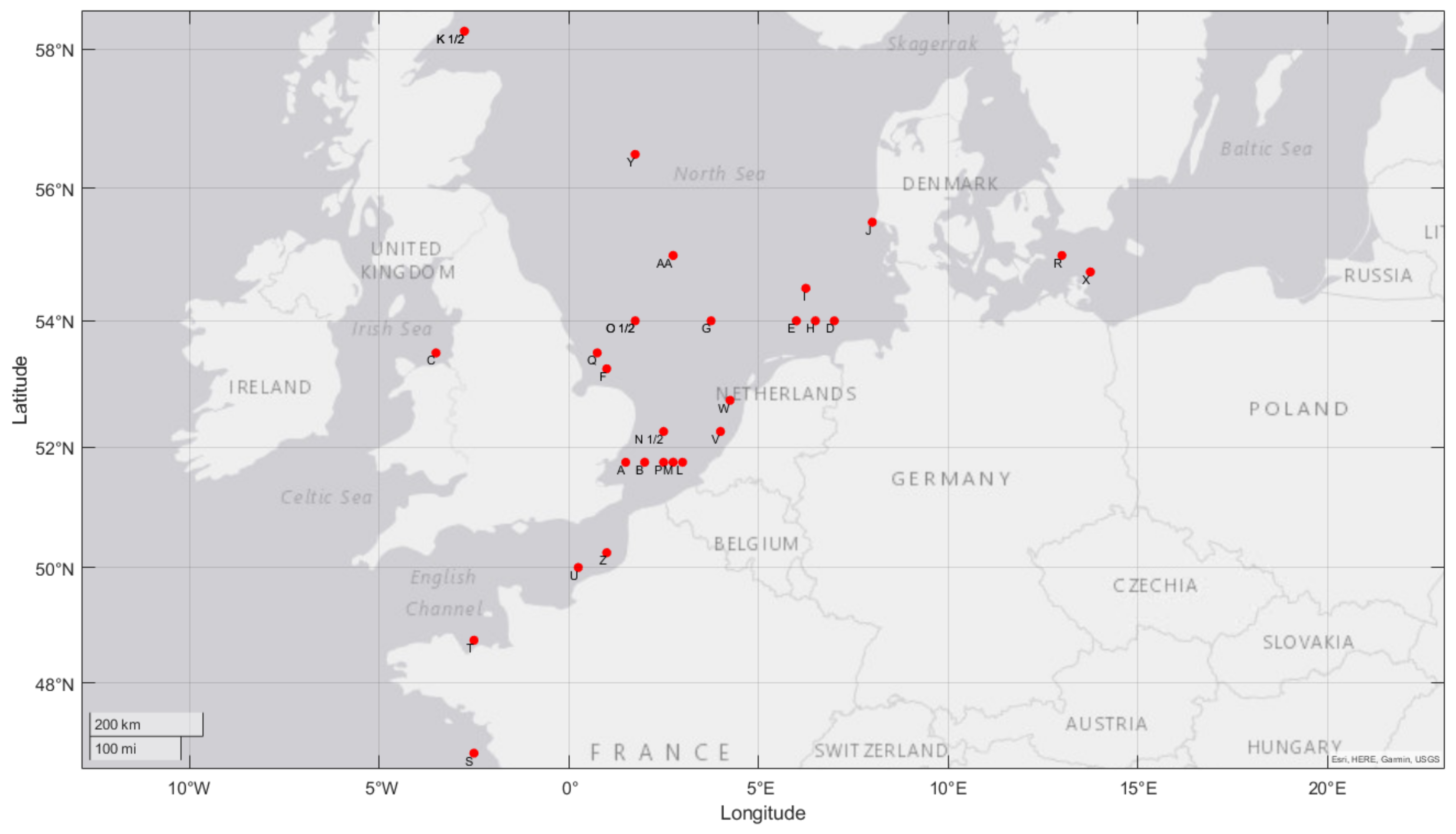
Figure 1. Map of Europe with locations of the 29 largest wind farms marked by red points. Large wind farms are mainly concentrated in the North Sea.
Energies 15 01700 g001
Figure 2. Wind roses for Gwynt y Mor and Kriegers Flak in 2019. Colors, from blue to red, indicate different wind speeds. Corresponding frequencies for each wind angle are displayed by the length of spokes.
Energies 15 01700 g002
Figure 3. Power curves and specific parameters of the two turbine types installed at Gwynt y Mor (SWT-3.6-107) and Kriegers Flak (SG 8.0-167 DD).
Energies 15 01700 g003
Figure 4. Generated power of different wind farms from 1 January 2019 to 31 December 2019.
Energies 15 01700 g004
Figure 5. Wind speed and power for Gwynt y Mor from 1 January 2019 to 31 January 2019.
Energies 15 01700 g005
Figure 6. Histograms of generated power from different wind farms in 2019.
Energies 15 01700 g006
Figure 7. Full-load hours of selected wind farms from 1980 to 2019. Every line illustrates the yearly full-load hours of one wind farm.
Energies 15 01700 g007
Figure 8. Correlation matrix of wind speed of considered wind farms. Shown are pairwise correlation coefficients, each calculated from the two vectors of hourly wind speeds from the respective sites. For clearer representation, the matrix elements are colored from dark blue (correlation is equal to 1 ) to dark red (correlation is equal to 1).
Energies 15 01700 g008
Figure 9. Pairwise correlation of wind speed vs. distance. Each point (blue) represents a pair of wind farms in the data. The best fitting exponential model ρ e x p ( d i s t a n c e / D ) is shown by the red line.
Energies 15 01700 g009
Figure 10. Correlation matrix of generated power of considered wind farms. Shown are pairwise correlation coefficients, each calculated from the two vectors of hourly production data from the respective sites. Again, for clearer representation, the matrix elements are colored from dark blue (correlation is equal to 1 ) to dark red (correlation is equal to 1).
Energies 15 01700 g010
Figure 11. Cumulative distribution function of total power generation in percent and corresponding 5% quantile in 2019. Note that the CDF starts with a zero slope at the beginning, illustrating that there are no hours without power production.
Energies 15 01700 g011
Figure 12. The 1%, 5%, and 10% quantiles of total power production from 1980 to 2019. Every line illustrates a quantile over the years derived from the yearly CDF of total power generation analogously to the CDF shown in Figure 11 for 2019.
Energies 15 01700 g012
Table 1. Considered wind farms in this paper. * Latitude in °North ** Longitude in °. Negative values refer to a position west of Greenwich; positive values refer to a position east of Greenwich. The placeholders ‘-’ mark the locations where reliable hub heights were not available (see text).
LetterWind FarmLat. *Long. **Hub (m)TurbineMWYear
ALondon Array51.751.587SWT-3.6-1206302012
BGreater Gabbard51.75278SWT-3.6-1075042012
CGwynt y Mor53.5−3.584.4SWT-3.6-1075762015
DGode Wind (1&2)547-SWT-6.0-1545822016
EGemini546120SWT-4.0.1306002017
FRace Bank53.251100SWT-6.0-1545732018
GWalney Extension543.75113V164-8.256592018
111SWT-7.0-154
HBorkum Riffgrund 1&2546.5-SWT-4.0-1207672019
-V164-9.0
IHohe See54.56.25105SWT-7.0-1544792019
JHorns Rev Phase 1–355.5870V80-2.07742019
68SWT-2.3-93
-V164-8.3
K1Beatrice58.25−2.7590SWT-7.0-1545882019
LBorssele Phase 1&251.753116.5SG 8.0-167 DD7522020
MSeamade51.752.75109SG 8.0-167 DD4872020
NEast Anglia One52.252.590.5SWT-7.0-1547142020
O1Hornsea (Project 1)541.75113SWT-7.0-15412182020
PBorssele Phase 3&451.752.5-V164-9.5731.52021
QTriton Knoll53.50.75105V164-9.58572021
RKriegers Flak5513104.5SG 8.0-167 DD6042021
O2Hornsea (Project 2)541.75123.5SG 8.0-167 DD13862022
K2Moray Firth (East)58.25−2.75122V164-9.59502022
SIles dYeu et de Noirmoutir46.75−2.5-SG 8.0-167 DD5002023
TBaie de Saint Brieuc48.75−2.5123.5SG 8.0-167 DD4962023
UHautes Falaises500.25-SWT-7.0-1545002023
VHollandse Kust Zuid52.254125.5SG 11.0-200 DD15002023
WHollandse Kust Noord52.754.25125.5SG 11.0-200 DD7592023
XBaltic Eagle54.7513.75107V174-9.54762023
YSeagreen56.51.75104V164-10.010752023
ZDieppe et Le Treport50.251-SG 8.0-167 DD4962024
AADogger Bank (Phase A, B)552.75150HALIADE-X 1324002024
Table 2. Descriptive statistics of wind farms in 2019.
Mean0.25-Q0.5-Q0.75-QSDR.-PowerFull-L.OffsNull
A309.2282.33264.52564.60235.60134242990629
B227.0750.65183.28420.21184.0166839460637
C232.8545.81175.18428.66202.2443135411789
D305.07103.43274.92569.18214.31182945912388
E424.30273.57502.65600.00193.22289461945137
F263.6868.66224.43504.85204.23145642303577
G351.81101.01353.45632.60249.42161447487557
H468.39223.50505.05759.62267.20216153981148
I279.68105.21294.44479.04180.07171649294330
J410.99146.14412.98706.55275.5283447290454
K1297.1778.12286.53533.44219.70125244272612
L420.03140.12442.84740.94285.04193248921568
M254.5082.42258.32452.66176.10186448041570
N342.6191.59302.09615.06261.90121342030566
O1669.02228.69690.831161.78452.20156948114425
P354.6496.78303.16643.89269.99134042461557
Q493.57129.64463.92873.43365.55111943344563
R342.72139.59389.24569.80212.61194452122458
O2814.13334.09975.331320.00496.632287540210413
K2613.67172.48619.161096.67438.12148546384577
S227.6247.77181.17428.48187.171249402012669
T236.3050.50191.57450.93190.38141341730639
U254.7148.05194.52484.49217.84124338400690
V809.81268.75763.131464.19568.92166346060458
W403.58132.63385.69721.04280.92159346570473
X254.7992.22255.60438.86171.12142046982428
Y553.12175.93558.39967.58383.88146146590480
Z240.0252.90203.74456.83190.66154742380670
AA1484.73602.791651.062469.39913.422171526530315
Total12,339.827429.5612,012.4617,489.415901.5844,71047049614,777
Publisher’s Note: MDPI stays neutral with regard to jurisdictional claims in published maps and institutional affiliations.

