1. Introduction
The electricity industry in the world has gone through significant transitions regarding the digitalization of electric networks, management and automation of industries, expansion in the use of renewable sources, and improvement of decentralized energy generation technologies. This process is synthesized in the so-called three Ds: decarbonization, digitization, and decentralization. In this context, Brazil, for example, has a privileged position, having, in 2020, about 83% of the electrical power system made up of renewable energy resources. However, it is worth noting that a considerable amount of these resources, about 65.2%, comes from hydroelectricity, whose expansion is limited due to solid environmental constraints. Thus, it is essential to optimize the operation of this type of resource, which is performed by operators and generation companies worldwide, mainly with the support of long, medium, and short-term generation scheduling (GS) models [
1]. The mathematical characteristics of these models are intrinsically linked to the market design employed in a given electrical system. In systems whose design adopts a loose-pool dispatch, the GS models are tools primarily used to maximize the expected revenue associated with energy trading in spot and future markets [
2,
3]. On the other hand, in the case of markets with centralized dispatch, i.e., the tight-pool, an independent system operator employs a chain of GS models to minimize the expected operating cost, considering some risk-measure [
4,
5,
6,
7].
Regardless of the market design, the representation of the hydroelectric production function (HPF) is a vital modeling aspect in each GS model. Briefly, the HPF relates the power output with the turbined outflow, net head, and efficiency. In turn, the generating unit (GU) efficiency is a function of the turbined outflow and net head. As a result, the HPF is usually represented by a two-variable, nonlinear, and nonconvex function. In addition to the representation by GU, the HPF can represent the plant generation by aggregating the GUs into an equivalent GU [
6]. In long and medium-term GS models, the inclusion of uncertainties for risk management via, for example, the stochastic programming model is a priority [
4]. In this case, the dimensionality and mathematical characteristics of the HPF must be controlled so that the models can efficiently include the uncertainties.
Furthermore, with the increasing insertion of wind generation and run-of-river hydroelectric plants, short-term GC models also include uncertainties in their modeling, demanding the same type of requirement as the more extended horizon models. In this context, the plant-based HPF is advantageous because the high dimensionality introduced by the individualized representation considerably increases the GS models’ computational burden. Although the plant-based representation is the most feasible option, other aspects that burden the solving strategies of GS models are the nonlinearities and nonconvexities inherent to the HPF. In this sense, an alternative that has proven to be very efficient is the HPF representation by a piecewise linear function (PWL), which allows GS problems to be effectively solved via state-of-the-art linear programming (LP) and mixed-integer linear programming (MILP) software.
The literature is very vast in the representation of HPF in GS problems. Thus, to support the developments proposed in this paper, in the sequence, we focused on more recent works that make use of the HPF aggregated representation, commonly called plant-based models. Thus, an efficient numerical optimization method to obtain an HPF is proposed for cascading reservoirs in long-term GS problems [
5]. The HPF depends on the average stored volume and the turbined outflow in this work. Despite the good accuracy of this method, the nonlinear representation of the hydraulic performance is not considered as in [
6]. Still, in [
6], the HPF was represented by a PWL model, which depends on the volume and the turbined outflow obtained by an algorithm incorporating convex hull (CH) techniques. This model is distinguished by using the nonlinear HPF instead of constant productivity models [
8,
9], whose HPF depends solely on the turbined outflow (therefore, it does not include the effects of the net head variations). Another common approach is the use of univariate PWL. In such a case, the gross head is fixed, and the linearization is accomplished for an HPF that depends on the turbined outflow [
7]. The main advantage of this method is the implementation’s simplicity and suitable computational performance. However, the non-consideration, simultaneously, of the net head and turbined outflow effects results in a flawed correspondence between the PWL and original HPF. Another alternative that can be used is the direct representation of the HPF by a set of concave functions dependent on the turbined outflow, according to [
9,
10]. However, this type of representation notably increases the number of constraints and variables in the problem.
The plant-based HPF is also widely used in the context of short-term GS models, whether in purely hydro systems [
11,
12,
13], hydrothermal systems [
14,
15,
16,
17,
18], or hydrothermal systems interconnected with renewable sources such as solar and wind [
14,
15,
16,
17]. In [
15], it PWL is obtained as a function of the turbined outflow and gross head through CH techniques. It is central to highlight that the resulting model obtained by the CH is concave. Therefore, the PLW can be included in the GS problems without adding binary variables, significantly favoring the computational performance. However, these approximations often overestimate the function, mainly in the nonconcave regions of the HPF, usually requiring coefficients adjustment or hybrid linearization strategies [
19]. The models proposed in [
14,
15,
16,
17] represent the HPF as a quadratic function dependent on the volume and the turbined outflow. Although the product between outflow and the net head has been included in this case, the use of quadratic functions inevitably leads to mixed-integer quadratic programming models (MIQP), which computationally burdens the resolution of the problem. The model proposed in [
16] used a nonlinear HPF depending on gross head and turbined flow. This approach requires the use of nonlinear programming (NLP) techniques that, although resulting in accurate solutions, are impractical for use in large-scale systems. Additionally, in some works, as in [
18,
20], the linearization is based on SOS2 sets. The idea is that the power generation, gross head, and turbined outflow can be expressed as a convex combination of SOS2 sets.
Some studies have relied on linearization based on the logarithmic aggregation convex combination (LACC) model [
19,
21]. According to the current literature, the LACC model represents one of the best options for representing high-precision PWL functions. However, the number of equations associated with LACC is intrinsically linked to the number of data points employed in the PWL approximation. This issue leads to incorporating more binary variables in CG models, further increasing the computational effort. In [
21], for handling this negative issue, the LACC is employed only in the nonconvex domain of the HPF, and the concave part is linearized by using CH techniques. Nevertheless, the overall PWL approach can often supply unnecessary equations for a given precision due to the lack of “controllability,” which is a key point we offer in this paper.
The primary purpose of this paper was to present a computational framework based on the most recent contributions developed for PWL fitting. A relevant particularity is that an analytical model is not available for the plant-based HPF, unlike the individualized case, unless some simplifications are adopted [
6,
22]. Thus, for the construction of the plant-based PWL, it must be considered that only a discrete set of points are provided, given by the triples (turbined outflow, gross head, and power generation) for the bivariate case where outflow and gross head are input parameters, or (outflow and power generation) for the univariate case where the gross head is fixed. In particular, the power generation values can only be obtained by solving a mixed-integer nonlinear optimization problem (MINLP) since the maximum power generation of the plant depends on which combination of GUs is used in the optimal dispatch [
23].
Recently, two studies presented significant contributions in PWL fitting [
24,
25], which avoids the use of nonlinear constraints necessary to preserve the continuity of the fitted model. Precisely, those works use big-M-type constructions to enforce continuity through a set of linear constraints. This paper aimed to use these formulations with modifications and contributions in the plant-based HPF.
Few papers in the literature propose a representation of the plant-based HPF with a PWL function obtained through a refined control of the number of hyperplanes or a pre-established linearization error. Therefore, the major contribution of this work is the “controllability” aspect. Our main objective was to present a computational framework based on the most recent contributions developed in PWL and apply it to the plant-based HPF. We also propose using the Ramer-Douglas-Peucker algorithm (RDP) [
26,
27] for the optimal selection of points to be used in the linearization process. Moreover, this approach also selects the nonlinear region of the HPF, which was our region of interest.
Firstly, this work showed the nonlinear HPF for the individualized case (i.e., GU), and then it built the optimization model based on MINLP to extract the plant-based HPF. The models then linearized the nonlinear HPF. In the proposed framework, the control is achieved in two ways: (i) minimizing the number of hyperplanes for a given error and (ii) minimizing the error for a fixed number of hyperplanes. By stipulating a given acceptable error in the linearization, it is possible to obtain the minimum amount of associated hyperplanes, thus limiting the number of variables in the problem and improving the computational performance. As a result of this, we can establish, for example, acceptable errors for different hydropower plants according to their importance in the system (e.g., power or storage capacity). The predictability of computational performance is improved if we choose to fix the number of hyperplanes, thus knowing the number of variables and constraints of the model in advance. The PWL models can still be restricted to produce nonconvex and concave PWL functions. Although more accurate, the nonconvex model requests binary variables, hindering use in large-scale problems. In this work, the nonconvex PWL was constrained to the univariate case, thus being more suitable for plants with lower capacity or simplified representation in the final stages of the planning horizon of a given GS model.
On the other hand, the concave PWL eliminates binary variables to represent the plant-based HPF. This paper used the concave approach in both univariate and bivariate cases. Subsequently, we presented two different methods of partitioning the HPF domain: (i) the most used in the literature which is based on uniform discretization, i.e., the domain is subdivided into a grid of equidistantly spaced points, and (ii) in which an optimal partition of the domain is performed using the RDP algorithm which, in general terms, searches for a curve with a higher concentration of points in regions of pronounced nonlinearity of the HPF. With the appropriate treatment of the data, the models proposed in this work then control the accuracy and the resulting computational effort in the GS models.
The remainder of this paper is organized as follows:
Section 2 provides details on obtaining the plant-based HPF.
Section 3 presents the proposed framework for the linearization of the HPF.
Section 4 presents the use of the RDP algorithm for the optimized pre-selection of data. Numerical results and discussions are provided in
Section 5. Finally, conclusions are discussed in
Section 6.
2. The Plant-Based Hydro Production Function
To present the plant-based HPF formulation, it is important first to detail the individual model, which is given by:
In (1),
gj is the power generation of the GU
j (MW),
gej is the global efficiency of the GU
j,
wj is the turbined outflow of the GU
j (m
3/s), and
hj is the net head of the GU
j (m). The net head is the difference between the gross head,
gh, and the hydraulic losses associated with the turbined outflow. By definition,
gh is given by the difference between the forebay and the tailrace levels, which depend in most cases on the stored volume (
v) and the total outflow (
d) of the reservoir, respectively, as follows:
In (2),
fbl(v) is the forebay level (m) and
tlr(d) is the tailrace level (m). The total outflow
d is given by
q +
s, where
q is the plant turbined outflow. Mathematically, the equation
represents the turbined outflow in the plant(m
3/s), and
s is the spillage (m
3/s). We momentarily put aside
fbl(v) and
trl(d) to write the HPF model with only two variables. The dependence of
gh with the forebay and tailrace levels is directly expressed in GS models as equality constraints or even as PWL. In that way, the net head is expressed as:
In (3),
Kj is the constant used to represent the hydraulic loss function in the GU
j (s²/m
5), which considers that the GU has an individual penstock. When this is not the case, (3) also depends on the turbined outflow of other GUs of the same plant. Although modeling (3) is the most common, the framework presented in this paper does not require this restriction. On the other hand,
gej in (1) includes several kinds of turbine and generator efficiencies (hydraulic, mechanical, and electrical). Based on field tests and hill-curve data from GU, a nonlinear function that depends mostly on
wj and
hj can express the global efficiency. We assume that the following polynomial function is available (although a different function can be used):
Above in (4),
Ekj is the
kth constant in the global efficiency function of the GU
j. By including (2) and (3) in (1), the unit-based HPF final expression is presented below.
As it can be seen, the expression (5) is written as a function of gh and wj because (3) only depends on wj. If this is not the case, then (5) must be written as a function of hj and wj.
Once the individual model is presented, the next step is to detail the plant-based model, the focus of this work. To do so, initially, consider that a given plant has
N GUs. To facilitate the presentation, also consider that each GU has only one operating zone, given by the range of the turbined outflow (W
jmin–W
jmax). Thus, to obtain the dimensional reduction aimed by the plant-based model, the
N individual HPF (5) must be replaced by a function that depends on
gh and the plant turbined outflow
q instead of
wj. As previously mentioned, an analytical and precise plant-based HPF is not available since the hydraulic loss and the global efficiency of the plant depend on the number of dispatched GUs for a given operating state (i.e.,
gh and
q). The alternative is to obtain a dataset of triples (
PGkl,
Qk,
GHl) based on the solution of the MINLP presented below. The MINLP considers as input the parameters the value of
Qk, for
k = 1,...,
K defined in (
Qjmin–
Qjmax) and
l =1,...,
L values of
GHl in the range (
HBmin–
HBmax).
In this optimization problem, k is the index associated with the plant turbined outflow Qk(m³/s), l is the index associated with the gross head GHl (m), PGkl is the power generation of the plant in (Qk, GHl), and uj is the binary indicating if the GU j is online (uj = 1) or offline (uj = 0). Notice that we are using uppercase bold notation for fixed values. Thus, K × L optimization problems are solved, and, therefore, we obtain K × L values of PGkl.
The objective function (6) maximizes the power generation by the plant. The constraint (7) delimits that the sum of the turbined outflow of the GUs is equal to the turbined outflow of the plant. The constraint (8) is the nonlinear nonconvex HPF related to the UG
j. Finally, (9) defines the limits of the turbined outflow of each GU, and (10) represents the integrality constraints. The (6)–(10) formulation describes the bivariate case since the HPF depends on
Qk and
GHl. Now consider the univariate case, where the gross head is fixed in
HB0, so we have a form dataset (
PGk,
Qk). The MINLP is now rewritten as:
The accuracy of the PWL depends on the number of points
K ×
L, such as
k = 1,...,
K and
l =1,...,
L (
L = 1 in the univariate case) points used in the proposed framework. In general, the quality of a PWL fitting increases with the increase in
K and
L. However, a fair value of the total points is not simple to determine, in particular, due to the nonconvexity of the HPF. Although the dataset obtained in the Formulations (6)–(10) and (11)–(15) can be used in the algorithms presented in
Section 3, it is possible to perform an optimized selection of these data using the Ramer-Douglas-Peucker (RDP) algorithm, as is shown in
Section 4. The RDP increases the computational performance, as it is possible to find a PWL model with equivalent precision using fewer points.
3. Piecewise Linear Models
The construction of the PWL models proposed in this paper was carried out using the methodologies [
19,
20] based on solving MILP or MIQP optimization problems. Thus, according to
Section 2, consider initially that (
PGkl,
Qk,
GHl) or (
PGk,
Qk) is available such that
k = 1,...,
K e
l =1,...,
L. Thus, we sought to determine a continuous PWL that best approximates this set of points, minimizing an error established by an
o-type norm. Considering formulations as parametric models, that is, the objective is to obtain coefficients that result in a set of multiple-choice hyperplanes [
28], the objective function of the PWL model optimization problem can be described for the univariate HPF, as follows:
In (16),
c1H is the slope or gradient 1 associated with
Qk in the hyperplane
H, and
dH is the linear coefficient associated with the hyperplane
H. The objective function (16) aims to minimize the
o-type norm of the sum difference between the approximate power generation of the hyperplane
H and the exact value of the nonlinear HPF,
PGk. Alternatively, for the bivariate case, we can rewrite the objective function as follows:
In (17),
c2H is the slope or gradient 2 associated with
GHl in the hyperplane
H. After the fitting process,
c1H,
c2H, and
dH will define the hyperplane
H of the PWL. The next subsections deal with the MILP and MIQP optimization problems used to determine them. The first subsection deals with the models and the algorithm for obtaining nonconvex and concave univariate PWL. In the second subsection, the models for obtaining the concave PWL are expanded to the bivariate case. The models presented in this work require the numerical values of the domains of the variables to be properly limited so that the models present a good computational performance. Furthermore, big-M parameters are extensively used to model linear constraints. For reference, check [
24].
Table 1 shows the summary of the models presented in this section. Checkmarks, “✓”, are for yes and “✕” are for no.
3.1. PWL Models for the Univariate Case
3.1.1. PWL Model 1
The PWL model 1 seeks to determine a PWL function for the univariate plant-based HPF. Consider the optimization problem (18)–(36) reformulated from [
24]:
In the optimization problem, B is the maximum number of breakpoints which is the first and last point of a line segment. The dimension of a hyperplane ∈ ℝ2 (our univariate case) has dimension 1 and therefore is a line segment Mka and Mk2 are the non-negative big-M parameters, δk,H is the binary variable that identifies which segment H each point k is associated with, C1H and are the minimum and maximum values of c1H, DH and are the minimum and maximum values of dH, δ+/−k,H are continuous variables that indicate whether there is a breakpoint between Qk e Qk+1, and yH is a binary variable that indicates the gradient change between adjacent linear segments.
The objective function (18) minimizes a chosen metric that, in this case, consists of the absolute error (o = 1) or the square error (o = 2); note that in the latter case, the model becomes a MIQP, which can considerably decrease the computational performance. The constraints (19) and (20) evaluate the approximation value at Qk. The constraint (21) ensures that each point k belongs to exactly one segment. The constraints (22)–(24) ensure the ordering of points in such a way that a point must be associated with the same or the next segment, where (23) and (24) ensures the ordering of the first and last data points, and (22) ensures the ordering of the other points. The PWL continuity is enforced through the constraints (25)–(30), which ensure that the breakpoint location, rH, is equal in adjacent segments regardless of the gradient change. In short, if cH − cH+1 > 0, it implies that yH = 1 and the constraints (27) and (28) are activated, which indicates that the gradient decreases between the two segments. Otherwise, if cH − cH+1 < 0, yH = 0, the constraints (29) and (30) are activated, which implies that the gradient increases between the two segments. Finally, if cH = cH+1, there is no breakpoint at that location, and the function remains with the same gradient. The constraint (31) ensures at least one equation for which the plant power generation will be 0 whenever the plant turbined outflow is 0. Finally, the constraints (32)–(36) define the domain of variables.
The MILP optimal solution is given by the coefficients (
c1H,
dH)/∀
H. However, since the resulting PWL is nonconvex, it is required that the location of each breakpoint,
rH, is known to delimit the domain for which each segment
H is valid. These values are implicitly modeled in the optimization problem to ensure continuity and reduce the number of variables. The breakpoints’ location can be calculated as:
Above, r1 and rB are the first and last breakpoint locations. For the other points, the location is calculated as in (38). Notice that if c1H = c1H+1, the model enforces dH = dH+1, which means that the two segments are affine with no discontinuity between (Qk e Qk+1); thus, rH can be chosen arbitrarily among these points.
3.1.2. PWL Model 2
The PWL model 2 has the same characteristics as Model 1 but with different strategies to establish the ordering and continuity of the function. Consider the optimization problem (40)–(56) reformulated from [
25]:
s.t.: (19)–(21), (31)–(34)
In this optimization problem, p+/−k,H and q+/−k,H are non-negative slack variables, uk,H is a binary variable that takes on the value 1 if p+k,H = q+k+1,H+1 = 0, vk,H is a binary variable that takes on the value 1 if p−k,H = q−k+1,H+1 = 0, δFk,H is a binary variable that assumes 1 if the point k is the first point in the segment H, and δLk,H is a binary variable that assumes 1 if point k is the last point of the segment H. Model 2 is identical to the model 1 concerning the objective function and constraints (19)–(21) and (31)–(34). The constraint (41)–(47) ensures the ordering, whereas (44)–(45) ensures the first and last points ordering of the data set. The ordering of the remaining points is handled via (46)–(47). The continuity of the HPF is enforced through the constraints (48)—(54). In this case, if a point is the last of the segment, (54) activates one of the binaries uk,H or vk,H that makes p+k,H and q+k,H = 0 or p−k,H e q−k+1,H+1 = 0. Thus, this ensures continuity through (48) and (49) by ensuring that, at this point, both functions result in a non-negative or non-positive value. Finally, the constraints (55) and (56) define the variables domain.
3.1.3. PWL Model 3
The PWL Model 3 adapts the alternative formulation of [
25] to minimize the number of breakpoints and, consequently, the number of segments for a given error.
s.t.: (21), (31)–(34), (41), (44)–(56)
In this optimization problem, WH is a binary variable that is 1 if H ∈ B is selected, Fk is a non-negative slack variable that only assumes a value greater than zero if the stipulated error Er cannot be achieved, and εk is the absolute error at point k. The objective function (57) minimizes the number of breakpoints plus the sum of non-negative slack variables. In conjunction with the constraint (60), the problem aims to minimize the number of breakpoints for a given stipulated error Er without using the slack variable (Fk = 0), zeroing the second term of the objective function. If Er cannot be achieved, then Fk > 0. The constraints (61) and (62) make δFk,H and δLk,H to be 0 for each inactive segment. The constraint (63) excludes some symmetric solutions. Lastly, constraints (64)–(66) delimit the domain of the introduced variables.
This formulation requires that a maximum value of breakpoints B large enough is defined so that an optimal solution lies within the range from 2 to B breakpoints.
There are cases where, depending on the region where the maximum error is observed, a maximum absolute error is required instead of having a low mean absolute error. If the error observed is in regions of interest of the HPF, it is possible to modify the constraint (60) and we can find a PWL as the slowest maximum absolute error for each point
k.
With the support of the slack variable Fk, it is possible to establish an algorithm (Algorithm 1) with a searching heuristic to obtain the lowest possible number of breakpoints for the lowest error achieved.
| Algorithm 1. The searching heuristic for the lowest number of breakpoints for a given error. |
1. Choose the total number of points K.
2. Get the plant-based HPF data set (PGk, Qk).
3. Choose the maximum number of breakpoints B.
4. Determine the metric-constraint (60) or (67).
5. Choose an initial value of Er and tolerance tol.
6. While Fk ≤ tol.Solve PWL Model 3.
7. Do Er = Er–0.01 (for 1% reduction per run)
8. Return the last set [c1H, dH], ∀H=1,…,B-1 which ∀Fk ≤ tol |
3.1.4. PWL Model 4
This section discusses the generalizations necessary to obtain a concave PWL. Unlike the nonconvex PWL functions in which it is necessary to use binary variables to indicate the domain of each segment within the GS problem, a given value of a concave function according to [
28] can be given by:
The objective function can be rewritten as:
A well-known property of concave functions is that:
Constraints (70) are equivalent to removing the term
of (19).
The concave formulation has strong symmetry, which results in identical equations from the permutation of the coefficients
c1H e
dH. The symmetry constraint (71) inhibits the existence of symmetric functions. However, it is worth noticing that the presence of constraint (71) might burden the model computationally so that it is advisable to treat the repeated coefficients externally. The presence of (70) makes the PWL models presented so far have solutions restricted to concave PWL. However, it makes several constraints in models 1, 2, and 3 unnecessary or redundant. Thus, the final formulation can be expressed as:
s.t.: (20), (21), (31)–(34) and (71)
Furthermore, relaxations of linear programming models that use big-M can have their performance improved if the following constraints are added to the model according to [
28]:
3.1.5. PWL Model 5
This model restricts the PWL of Model 3 to concave functions.
s.t: (21), (31)–(34), (41), (44)–(47), (59)–(63), (71), (73)–(75)
The optimization problem above returns a concave PWL with the number of approximations less than
B, given the stipulated mean absolute error
Er. It is also possible to establish an algorithm (Algorithm 2) that seeks the lowest number of breakpoints for the lowest error reached, as carried out for the MLP 3.
| Algorithm 2. The searching heuristic for the lowest number of breakpoints for a given error for the concave case. |
1. Choose the total number of points K.
2. Get the plant-based HPF data set (PGk, Qk).
3. Choose the maximum number of breakpoints B.
4. Determine the metric-constraint (60) or (67).
5. Choose an initial value of Er and tolerance tol.
6. While Fk ≤ tol.Solve PWL Model 5.
7. Do Er = Er–0.01 (for 1% reduction per run)
8. Return the last set [c1H, dH ], ∀H=1,…,B-1 which ∀Fk ≤ tol |
3.2. PWL Models for the Bivariate Case
3.2.1. PWL Model 6
The PWL model 6 is intended to be used in the bivariate plant-based HPF, and it is an expansion of model 4. In the bivariate case, in addition to the coefficient,
c1H, associated with turbined outflow
Qk, it is necessary to calculate the coefficients
c2H associated with the gross head
GHl. Note that, in the bivariate case, the HPF consists of hyperplanes
H ∈ ℝ
3 with its domain delimited by two variables, and therefore each approximation is the equation of a plane. The formulation to obtain the bivariate concave PWL is expressed as follows:
s.t: (31)–(33), (63),(64),(71)
In the optimization problem, NH is the maximum number of hyperplanes, C2H, and are the minimum and maximum values of c2H. The objective function (78) minimizes the chosen metric, the absolute error (o = 1) or the square error (o = 2). The constraints (79) and (80) evaluate the approximation value at the point (Qk, HBl). The constraint (79) also imposes concavity requirements. Constraint (81) ensures that each point belongs to only one plane. The constraints (82) add a second requirement (first, being (31)) to ensure that there is a plane only Q-dependent so that the HPF returns a power generation 0 for any situation where Q = 0. The constraints (83) and (84) improve the model’s computational performance. Finally, (85)–(86) delimit the domain of variables.
3.2.2. PWL Model 7
The PWL model 7 expands the PWL model 5 to the bivariate case. In this model, the objective is to minimize the number of planes for a certain pre-established error.
s.t: (31)–(33), (71), (79)–(86)
At last, it is also possible to establish a search algorithm (Algorithm 3) for the formulation (87)–(96).
| Algorithm 3. The searching heuristic for the lowest number of breakpoints for a given error for the bivariate concave case. |
1. Choose the total number of points K and L.
2. Get the plant-based HPF data set (PGkl, GHl, Qk).
3. Choose the maximum number of hyperplanes NH.
4. Determine the metric-constraint (95) or (67).
5. Choose an initial value of Er and tolerance tol.
6. While Fkl ≤ tol.Solve PWL Model 7.
7. Do Er = Er–0.01 (for 1% reduction per run)
8. Return the last set [c1H, c2H, dH ], ∀H=1,…,B-1 which Fkl ≤ tol |
3.3. Solution Quality Evaluation
After obtaining the PWL through the PWL model, it is necessary to measure the respective quality. The objective function of some of the proposed formulations returns the error, but only concerning the points used as a reference in obtaining the approximations. Thus, the PWL test for a larger data set is proposed to test the segments or planes obtained. This accuracy evaluation is performed by using the maximum absolute (97) and the mean absolute error (98).
In the optimization problem, n is the index for data point being tested, N is the number of data points, PGn is the power generation at point n, Pn is the power generation at point n obtained by employing the PWL, MAE is the mean absolute error, and MAX_A is the maximum absolute error. Therefore, we employ a large number of N points for accuracy assessment.
5. Experimental Results
The models were implemented in python, embedded with GUROBI version 8.1.1. The codes were run on an Intel 2.5 GHz machine with 8 GB of RAM. The data sets were taken from two Hydropower Plant (HP) in Brazil: Santo Antônio Hydropower Plant (SAHP) and Machadinho Hydropower Plant (MAHP).
SAHP is the fifth-biggest hydropower plant in Brazil, with a total capacity of 3568 MW. The SAHP possesses 50 bulb turbines allocated into two groups: 24 four-blade with 73.29 MW and 26 five-blade with 69.59 MW, each group with a specific hydraulic efficiency curve.
Table 2 describes the operating limits for the GUs.
On the other hand, the MAHP has three identical GUs with a 380 MW capacity.
Table 3 shows the operating limits for the MAHP GUs.
Section 5.1 analyzes the PWL models 1, 2, and 4 for fitting univariable discrete data with a predetermined number of breakpoints. In
Section 5.2, the nonconvex and concave PWL functions are evaluated for the number of breakpoints minimization by employing the PWL models 3 and 5 (Algorithm 1 and Algorithm 2, respectively). Finally, in
Section 5.3, we analyze the approaches intended for the bivariate case with a predefined number of planes.
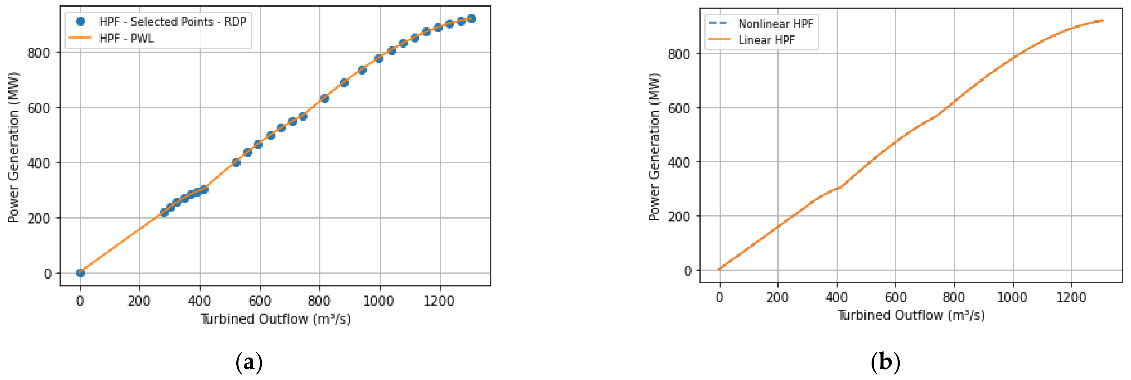
5.1. PWL Models 1, 2 and 4
The optimization model (11)–(15) was first used to obtain K = 1000 points (Qk, PGk) with GH = 100 m for MHP and GH =15 m for SAHP. The RDP algorithm was then used for optimal discretization. The resulting dataset was then applied to models 1, 2, and 4 to obtain the PWL. The number of breakpoints B was fixed at 10, which resulted in nine segments. Finally, the evaluation was verified using the objective function value (sum of the absolute difference, where o = 1), the maximum absolute error, and mean absolute error (97) and (98) for N = 1000 points (Qn, PGn).
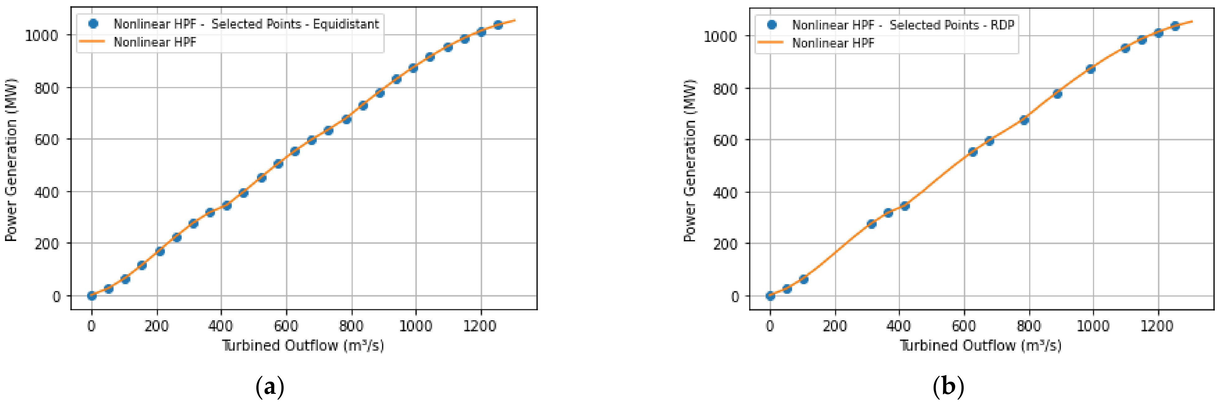
When applied to the 1000 initial points, the RDP algorithm selected 27 and 17 points (
Qk,
PGk), respectively, for MHP and SAHP with ε = 0.5 MW.
Figure 3a shows the points selected from the nonlinear HPF by the RDP algorithm and the behavior of model 1.
Figure 3b illustrates the approximation behavior for the 1000 test points.
Note that there is a region below 280 m³/s in the nonlinear HPF in which no points were selected since it refers to the GU forbidden zone. In this case, a turbined outflow between 0 and 280 m³/s cannot be supplied by the plant since even if the plant uses a single GU, this value would still be below the operating limits.
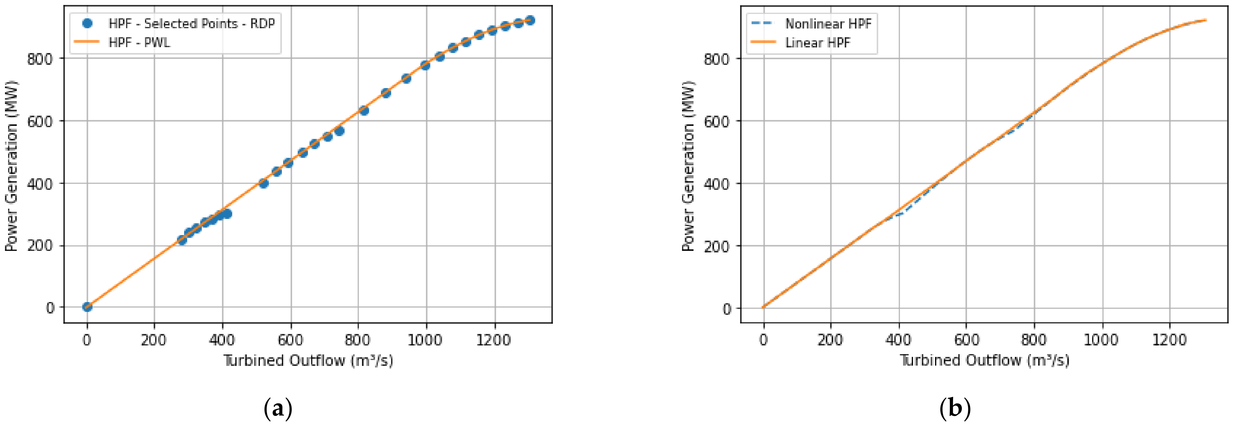
Figure 4 shows the curves obtained for the same data set for the PWL model 4 (concave approach).
Table 4 summarizes the three formulations applied to the MAHP.
Regarding the models that generate nonconcave PWL functions, model 2 showed slightly better accuracy results. Model 1 proved to be superior in terms of time simulation time, which is expected, considering that model 2 presents a greater number of variables and constraints. However, it should be noted that if the linearization process is not embedded in the GS model, the simulation time factor may be negligible since it will be performed only once (offline). It is important to point out that the PWL model 2 did not always show better accuracy than model 1, and, therefore, it is advisable to run both models every time and choose the one that best fits the data.
It is worth mentioning that accuracy might improve for a different number of B and if the RDP tolerance ε is narrowed. This action, however, would increase the running time of the model.
As a consequence of the concavity requirement, the PWL model 4 presented an error higher than the nonconvex models; however, it can be applied in GS models without binary variables. For group 2 of SAHP, model 2 yielded the behavior as seen in
Figure 5.
Table 5 and
Table 6 summarize the results for the three models applied to both groups of SAHP.
First, in general, the results were better for SAHP than MAHP. That is explained by the behavior of the nonlinear HPF of the latter. The more GUs a hydropower plant has, the more linear the plant-based HPF is expected to be, which directly impacts both precision and performance. The great linearity also explains the large exclusion of points in the intermediate (more linear) region.
The running time of model 2 was higher than model 1, again, explained by the high number of constraints and variables. In terms of accuracy, model 1 and 2 presented a very close mean absolute error for both groups, with model 2 presenting a slightly better accuracy for the mean and maximum absolute error in group 1 of SAHP. Once more, the variance in terms of accuracy justifies the use of both models.
Both groups of SAHP showed a better mean absolute error than the MAHP but with a worse maximum absolute error. This performance is explained by the lower operational limit of the generating units of SAHP, where any difference in lower values of the curve incurs a bigger maximum absolute error. It is also worth noticing that the objective function minimized the mean absolute error for the given examples.
Despite reducing the number of variables and constraints concerning nonconvex models, we noticed in some simulations that the computational performance could sometimes be worse in concave models. This aspect is because the concavity condition constrains the breakpoints’ location. On the other hand, the accuracy will always be equal (if nonlinear HPF is concave) or lower than those obtained in nonconvex models, mainly due to the error increasing in the nonconcave regions of the HPF.
5.2. PWL Models 3 and 5
For this type of analysis, the optimization model (11)–(15) is first used to obtain K = 1000 points (Qk, PGk) with the GH = 100 m for MAHP and 15 m for SAHP. The RDP algorithm was then used for optimal discretization. The maximum number of breakpoints was stipulated as the maximum number of points obtained by the RDP (27 in MAHP and 17 in SAHP). Additionally, we considered Er = 0.25 for the initial absolute error. Finally, Algorithm 1 and Algorithm 2 were applied to obtain the minimum breakpoints.
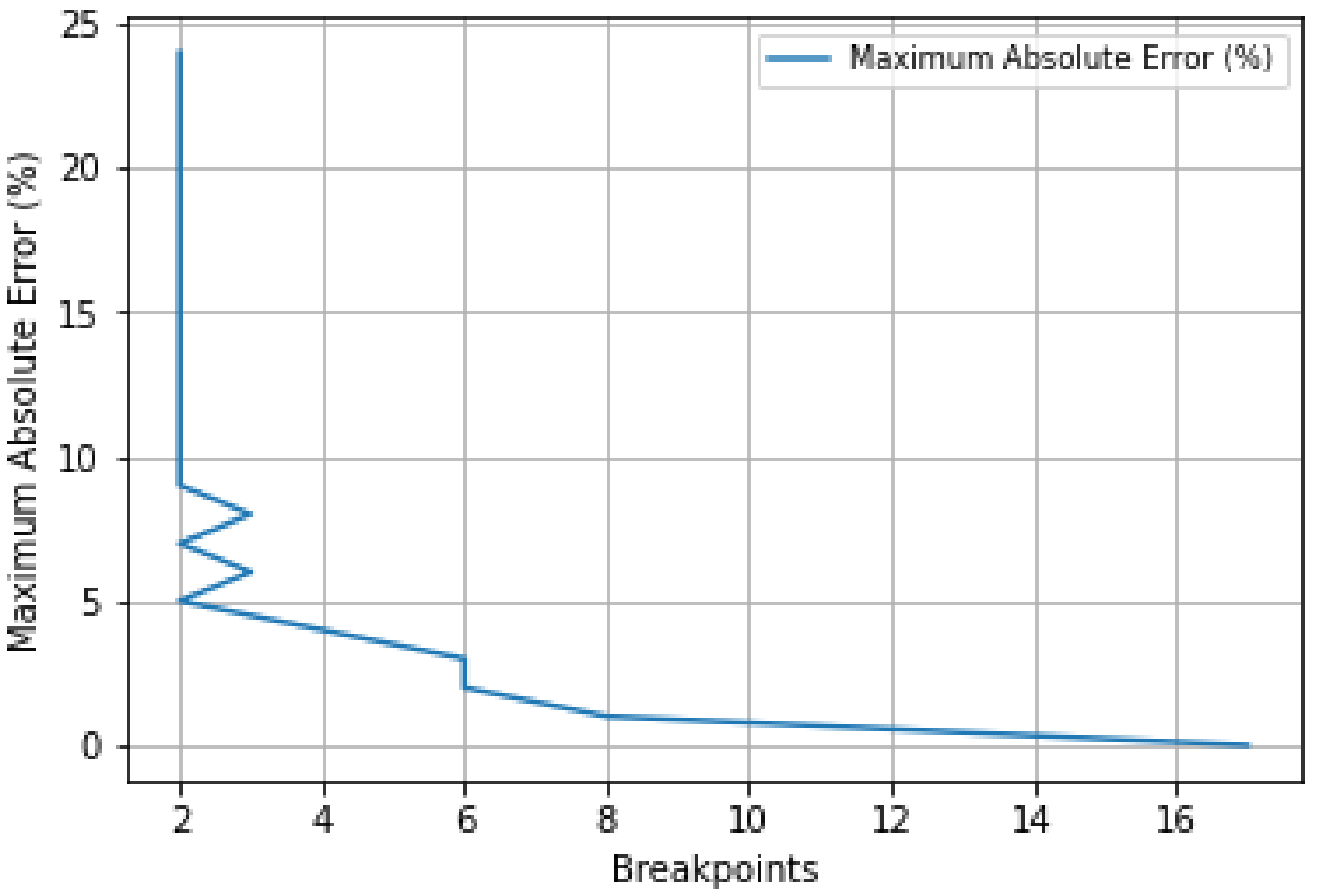
Figure 6 illustrates the progression of Algorithm 1 to reduce the maximum absolute error, using model 3 for MAHP. As can be seen, the error started at 25% with two breakpoints, reaching the optimal maximum absolute error at 0.7% with 17 breakpoints.
Table 7 summarizes the results obtained for both models.
Since we chose the maximum absolute error as the metric, it was observed that at the optimal number of 17 breakpoints, the maximum absolute error was better than at the fixed value of 10 breakpoints in
Section 5.1.
Table 8 and
Table 9 summarize the results for Algorithm 1 for SAHP.
Algorithm 1, using PWL model 3, found an optimal solution of 0.341% and 0.306% for SAHP groups 1 and 2, respectively, with 19 breakpoints in both. Like MAHP, the mean absolute error was penalized when using the maximum absolute error as the stipulated error. Algorithm 2, using PWL model 5, found 2.589% and 2.410% maximum absolute error with four breakpoints.
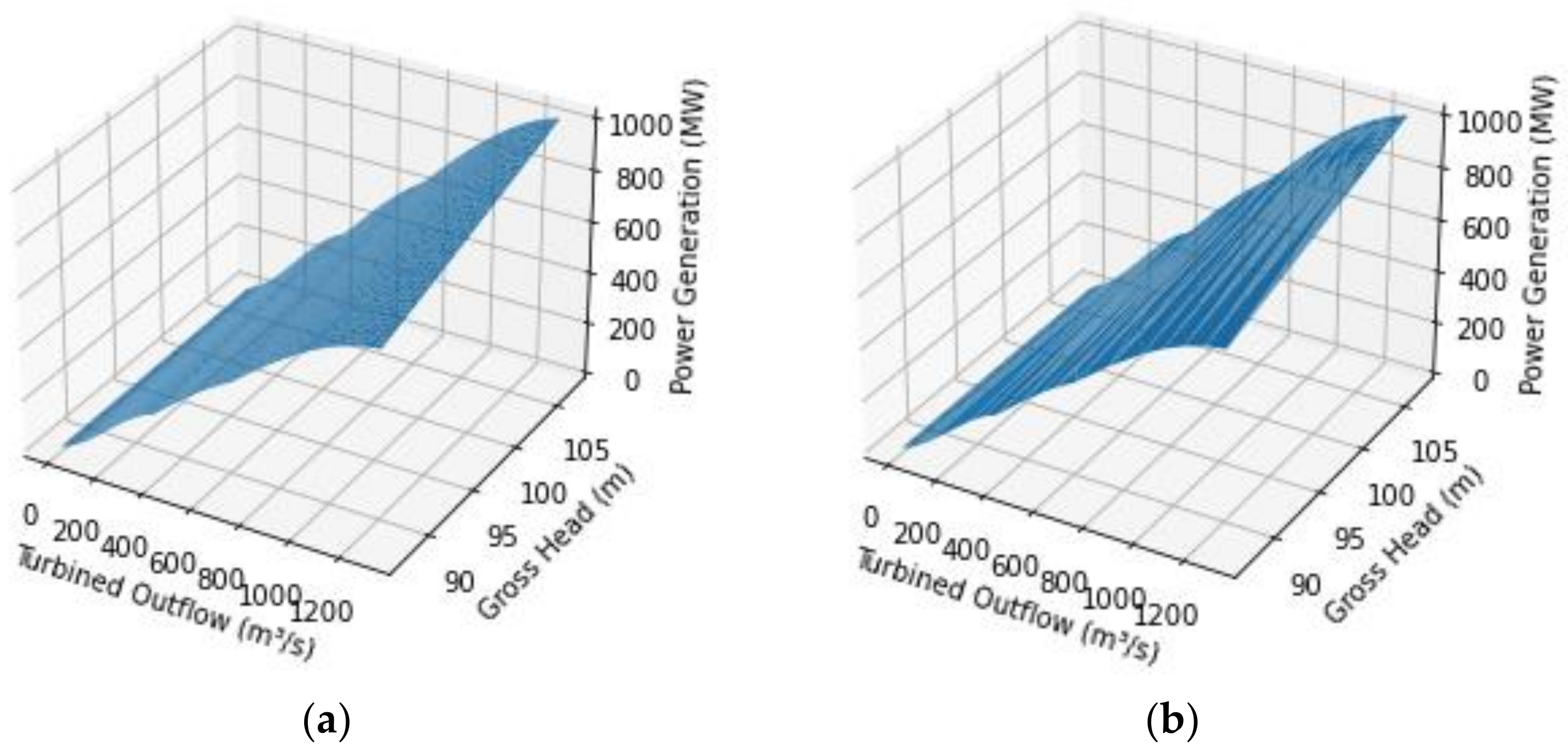
5.3. Analysis of Models 6 and 7
The PWL models 6 and 7 are proposed to the bivariate case. The optimization model (6)–(10) was first used to obtain the dataset, with
K = 100 and
L = 100, which resulted in 10,000 points (
Qk,
GHl,
PGk). The RDP algorithm was used for optimal discretization of the points. The number of
NH planes was set at 10 for formulation 6. Finally, the evaluation was performed similarly to
Section 5.1 and
Section 5.2, but the PWL was tested for 10,000 data points.
For formulation 7, the maximum number of planes was stipulated as the maximum number of points obtained by the RDP and the initial error Er = 0.25 (25%) for the maximum absolute error. Then, algorithm 3 was applied to obtain the minimum number of planes.
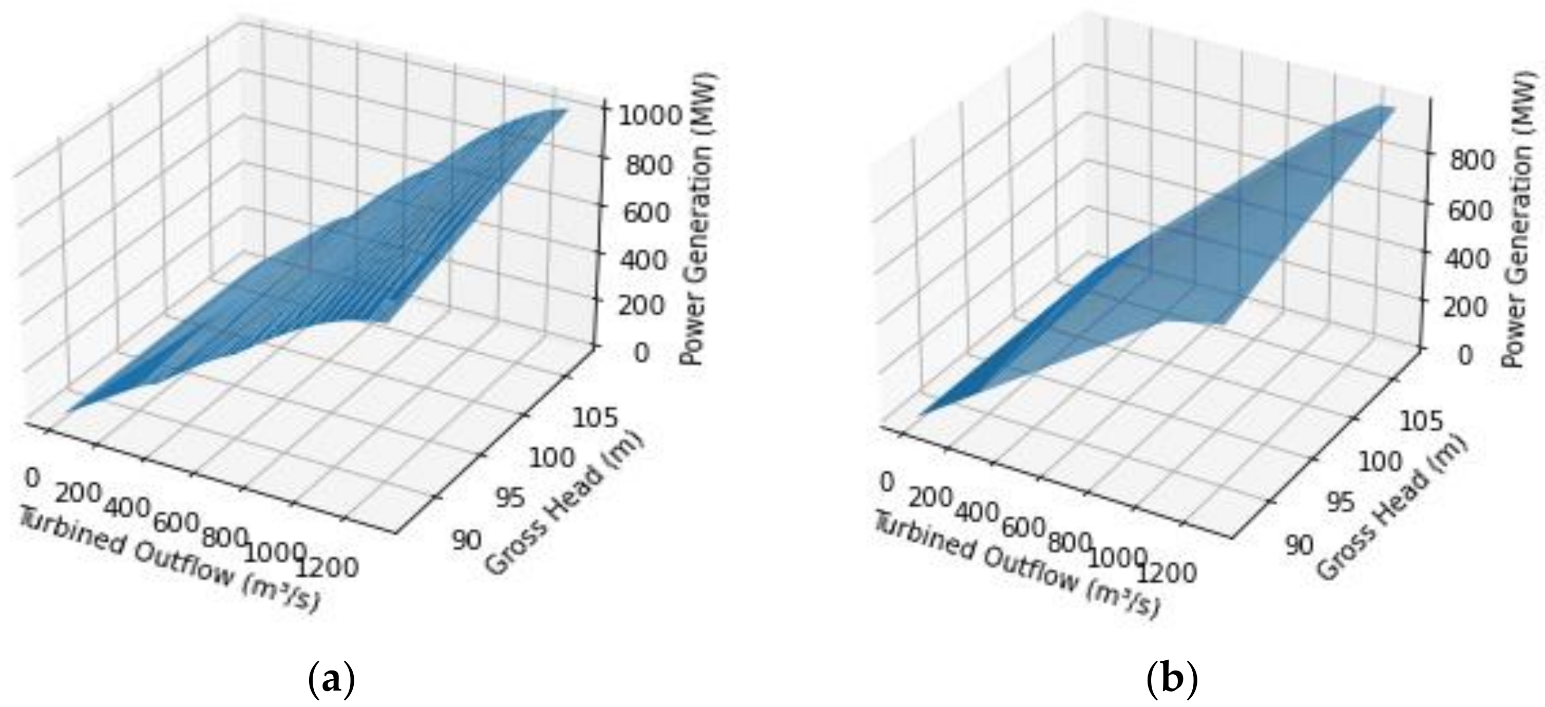
Applying the PWL model 6 for MAHP, we observed the following curve in
Figure 7.
Table 10 summarizes the results obtained with model 6.
As seen, in general, with more variables it is usual to observe a worsening of the precision. However, the mean absolute error was reasonable even for the bivariate case. The model convergence improved considerably since adding one more gradient added some malleability when obtaining the approximations. Using Algorithm 3, we noticed the following progressions for group 1 of SAHP.
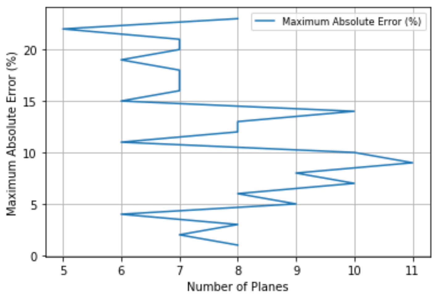
The performance of Algorithm 3 applied to SAHP is presented in
Figure 8, which stopped at 2.970% maximum absolute error to the reference points. Additionally, it resulted in 4.680% when applied to the 10,000 test points.
Table 11 summarizes the results obtained with model 6.
It was observed that just as in the univariate case, the maximum absolute error was improved at the cost of worsening the average absolute error.
Even in the bivariate case, the computational time was good due to the freedom in the number of hyperplanes chosen. Note that despite the algorithm being an iterative process, the computational time to determine the optimal number of hyperplanes for a given error was relatively fast, considering that Model 7 has a short running time.


