CFD-Based Erosion and Corrosion Modeling of a Pipeline with CO₂-Containing Gas–Water Two-Phase Flow

Abstract

A natural gas transportation pipeline with a gas–water two-phase flow containing CO₂ is prone to severe flow-assisted corrosion (FAC). The accumulation location of the water phase in the pipeline and the wall shear stress distribution are important factors affecting the severity of this phenomenon. In this work, computational fluid dynamics (CFD) simulations were performed using the realizable k-ε model and volume of fluid (VOF) model to determine the gas–water volume fraction distribution and wall shear stress in a gas–water two-phase pipeline and established a pipeline corrosion prediction model. By determining where the water phase accumulates in the pipeline, the potential corrosion area could be predicted. By alleviating the phenomena of excessive local wall shear stress and bubble cavitation, the FAC due to the formation of stress and acid gas can be controlled. The simulation results lay a certain foundation for the corrosion research of gas–liquid two-phase flow pipelines.

1. Introduction

Pipeline transport is an important mode of transportation in the oil and gas industry owing to its good economy and safety [1,2]. However, with the progress of mining, the natural gas mining environment has become harsh, and pipeline operations are accompanied by the production of acid gas and water [3]. Without dehydration treatment, the local water content in the pipelines can reach 90%, which leads to a corrosive environment [4].

The water distribution in the pipeline has an important influence on pipeline corrosion [5]. The presence of water and acid gas inside the pipeline is a prerequisite for internal corrosion [6,7]. Any direct contact between the accumulated water layer and the pipeline can cause internal corrosion, whereas no such phenomenon is observed in the case of discrete phase water. Therefore, when predicting corrosion in a pipeline, it is important to accurately determine the distribution of the water in the pipeline. So far, studies have been conducted on oil–water two-phase flows, with few researchers attempting to study the corrosion behavior of gas–water two-phase flows [4,8,9]. The fluid flow velocity of natural gas pipelines is typically high, and the flow patterns vary. Therefore, it is necessary to use computational fluid dynamics (CFD) models to predict the characteristics of the gas–water two-phase flow in natural gas pipelines. CFD theory uses computers to solve partial differential equations of fluid flow, and then studies fluid flow phenomena and related characteristics through flow fields and other physical fields. The widely used numerical calculation methods are the finite difference method, the finite element method (FEM), the boundary element method, the finite volume method and the finite analysis method. Through the comparative analysis, it can be seen that the FEM has attracted the attention of researchers because of its high calculation accuracy and good effect of complex boundary processing. At present, the software applied to the FEM method are ABAQUS, ANSYS and MSC. Among them, ANSYS software is composed of a whole set of extensible, flexible and integrated modules, which can meet various engineering needs. When ANSYS is used for numerical analysis of gas–water two-phase flow, the selection of models is very important, which mainly includes turbulent flow model and multiphase flow model. Many researchers have conducted in-depth research on turbulence models [10,11,12], and the differences between turbulence models are shown in

Table 1. Comparative analysis of turbulence models.

Model	Characteristic	Applicable
Standard k-ε	Moderate calculation and high precision	Fully turbulent
RNG k-ε		Transient or streamline bending flows
Realizable k-ε		Rotary or separation flows
k-ω	Moderate calculation and precision	Wall bound or free shear flows
Large eddy Simulation (LES)	Large calculation and high precision	Vortex flow
Reynolds stress model (RSM)	High precision	Strong vortex or hurricane flows

. The comparative analysis shows that the realizable k-ε equation not only has the advantages of a small calculation amount and high calculation accuracy, but also can effectively solve the problems of rotating flow and separation flow, so it has been used in project research by many researchers. In addition, the multinomial flow model also has a serious impact on the analysis results [13,14]. ANSYS software provides three multinomial flow models, the VOF model, the Euler model and the mixture model, respectively. To be able to track the interfacial separation phenomenon in the gas–liquid two-phase flow process, the VOF model is more suitable, and this conclusion can be obtained from the previous literature [15].

The steel that is used to make such pipelines is subjected not only to electrochemical corrosion during natural gas transportation, but also to mechanical erosion. This leads to accelerated corrosion and risk of failure, which is called flow-assisted corrosion (FAC) [16,17]. Islam and Farhat [18] pointed out that FAC has a significant influence on the corrosion and failure of pipeline materials. Particularly at elbows, reducers, and T-shaped pipes, the shear stress generated by the flowing gas destroys the protective film on the metal surface [18,19,20]. The FAC behavior at different elbow positions is different [21,22] due to the change in the water flow direction and velocity. A high-velocity fluid can damage the protective film and even damage the metal surface. However, the FAC of a natural gas pipeline is significantly different from liquid–solid two-phase flow corrosion and multiphase flow corrosion. In an actual pipeline transport process, because of the change in the elbow angle, each part of the pipeline exhibits a water hammer phenomenon to different extents, causing a change in the wall shear stress [23,24,25]. Most natural gas pipeline failures occur in these areas. However, research on this topic is limited. Therefore, it is necessary to study the influence of FAC on the natural gas transportation process, particularly the effects of fluid velocity and elbow angle.

In this study, a CFD model was used to study the water-phase wetting conditions in gas–water two-phase natural gas pipelines, and the effect of FAC was analyzed in terms of the effects of fluid velocity and elbow angle on the wall shear stress. This study provides a theoretical basis for the safety of natural gas pipelines.

2. Methodology

2.1. Operating Parameters

The flowing medium in the pipeline was a gas–water two-phase fluid, in which CO₂ was dissolved in the water [26]. Considering the actual working conditions of natural gas pipelines, the dissolved CO₂ in the pipeline transportation fluid was significantly lower than the saturation level [4]. Figure 1 shows the physical model of the natural gas pipeline. Three physical models were selected for the simulation calculations: an upward-inclined pipeline (case 1), a straight horizontal pipeline (case 2), and a downward-inclined pipeline (case 3). The inclination angle in both the upward and downward cases was 30°. The pipeline diameter was 300 mm, and the total effective length of the pipeline was 5000 mm. The gas superficial velocity considered in the pipelines were 0.5, 1, 3, and 5 m/s. The gas–water volume percentage was as follows: 90% water–10% gas, 70% water–30% gas, 50% water–50% gas, 30% water–70% gas, and 10% water–90% gas. The temperature was set to 20 °C, and the operating pressure was set to 3 MPa.

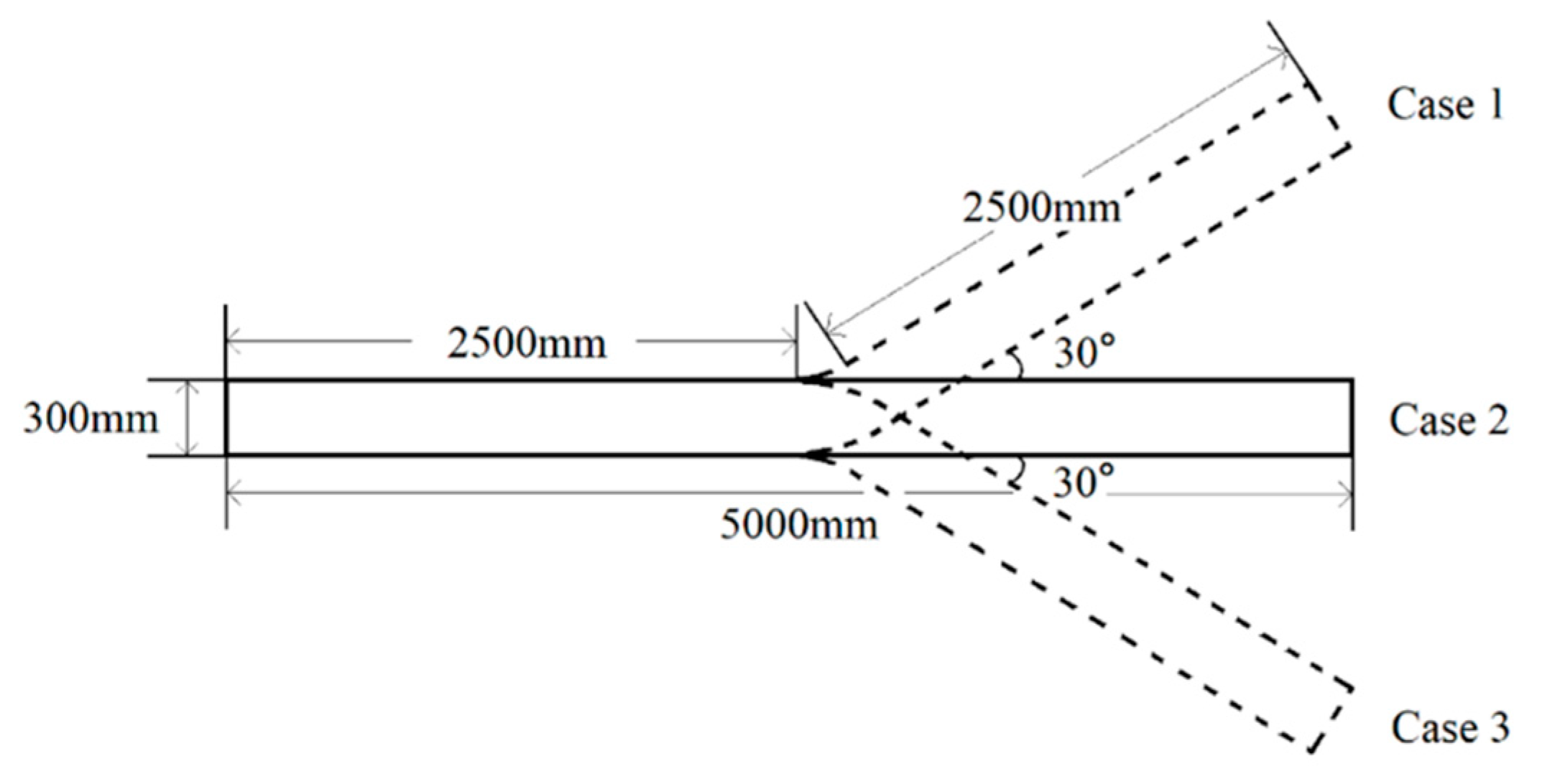
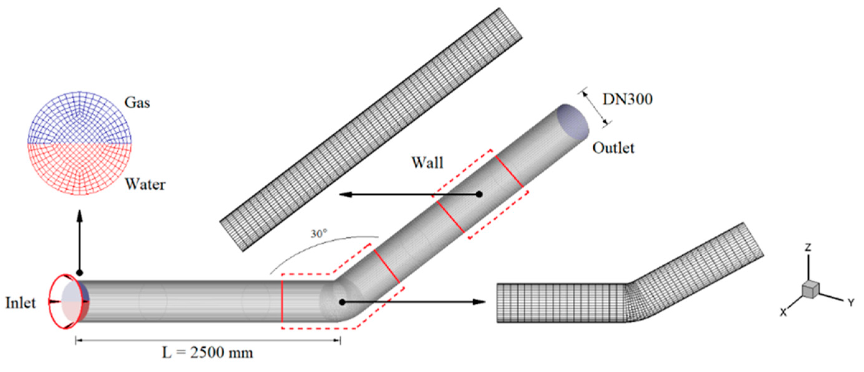
2.2. Meshing and Modeling

The ANSYS ICEM CFD software was used for physical modeling and structured meshing of the pipeline. The structured mesh was chosen as it can provide high-quality solutions with a small number of cells [27]. Figure 2 shows the meshing result of the physical model of the upward-inclined pipeline (30°).

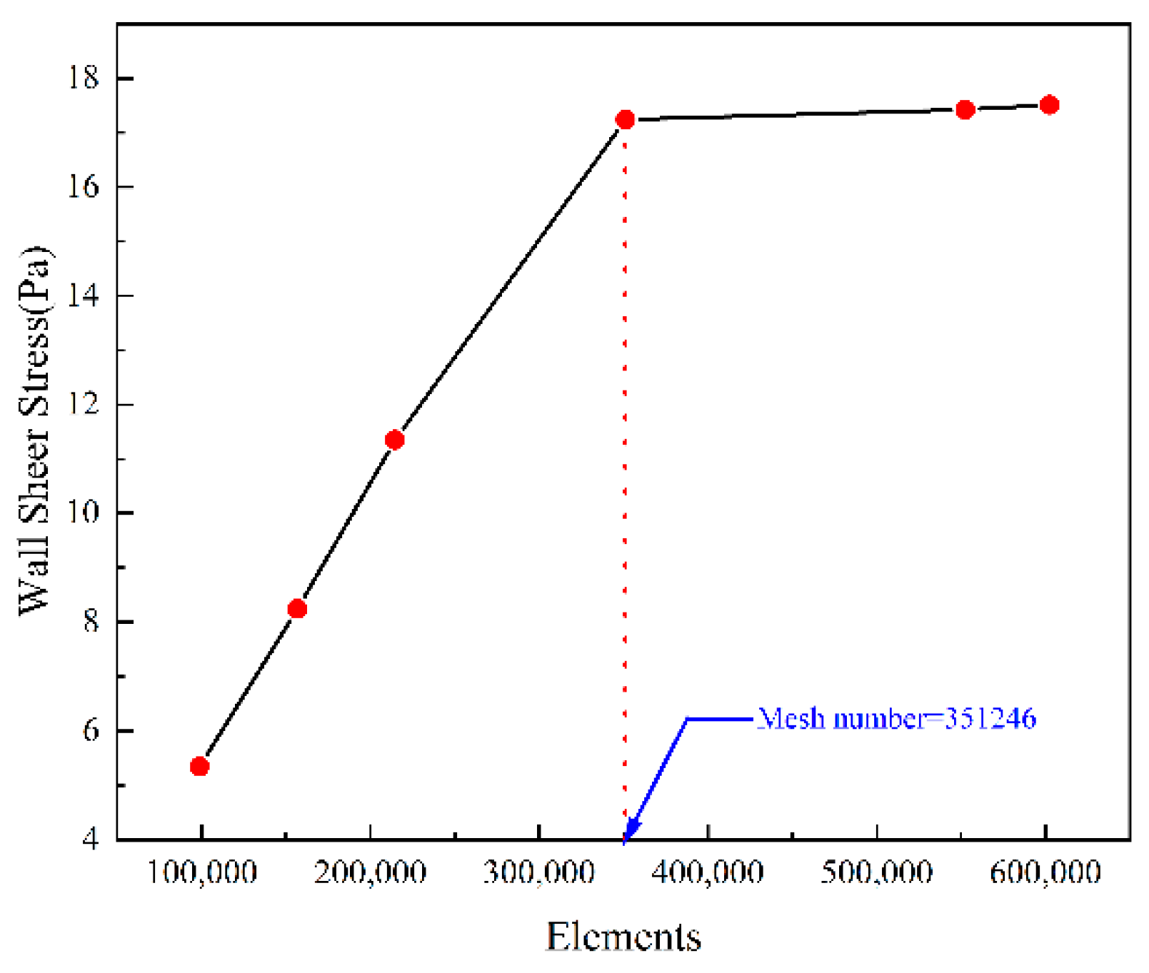
2.3. Mesh Independence Test

To obtain a sufficient mesh density to ensure the calculation accuracy, the mesh independence was verified. A pipeline with a gas superficial velocity of 0.2 m/s and 50% gas–50% water was taken as an example for analysis. Figure 3 shows the effect of the number of meshes on the maximum wall shear stress. As shown, when the number of meshes is <351,246, the maximum wall shear stress reaches the peak point, and the calculated stress for mesh numbers greater than this value is approximately the same. Therefore, this mesh setting is selected as the best working condition for the CFD simulation.

2.4. Assumptions and Initial Conditions

The CFD simulation process was conducted using ANSYS FLUENT 2019 software. In the simulation calculation process, the fluid flow was considered as transient, and the influence of temperature fluctuations on the fluid flow was negligible; therefore, the phase change and mass transfer between phases were not considered [28,29]. Assuming that the fluid at the pipe wall was stagnant [30], it is defined using a standard wall function (y⁺ = 30). The realizable k-ε turbulence model was selected for the simulation calculation. In order to better identify the gas–water interface and judge the position of water accumulation in the pipeline, the VOF model is used for simulation calculation. The boundary conditions for the velocity inlet are set at the inlet of the pipe, the boundary conditions for the pressure outlet are set at the outlet of the pipe, and the boundary conditions for the wall area are set in combination with the fluid and solid areas.

In the calculation process, the relaxation factors were all set to 0.3 and the flow parameters were calculated using the second-order upwind discrete scheme. In the calculation process, the first criterion is whether the residuals converge. The transient simulation process included 200 time steps; the time step length was 0.05, and 100 iterations were performed in each time step.

3. Results

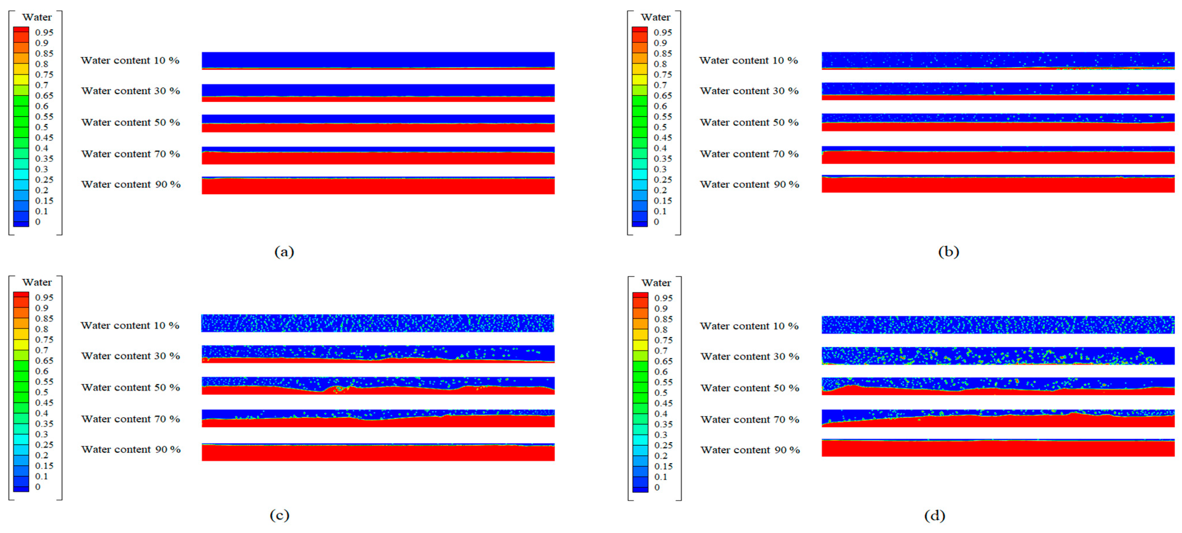
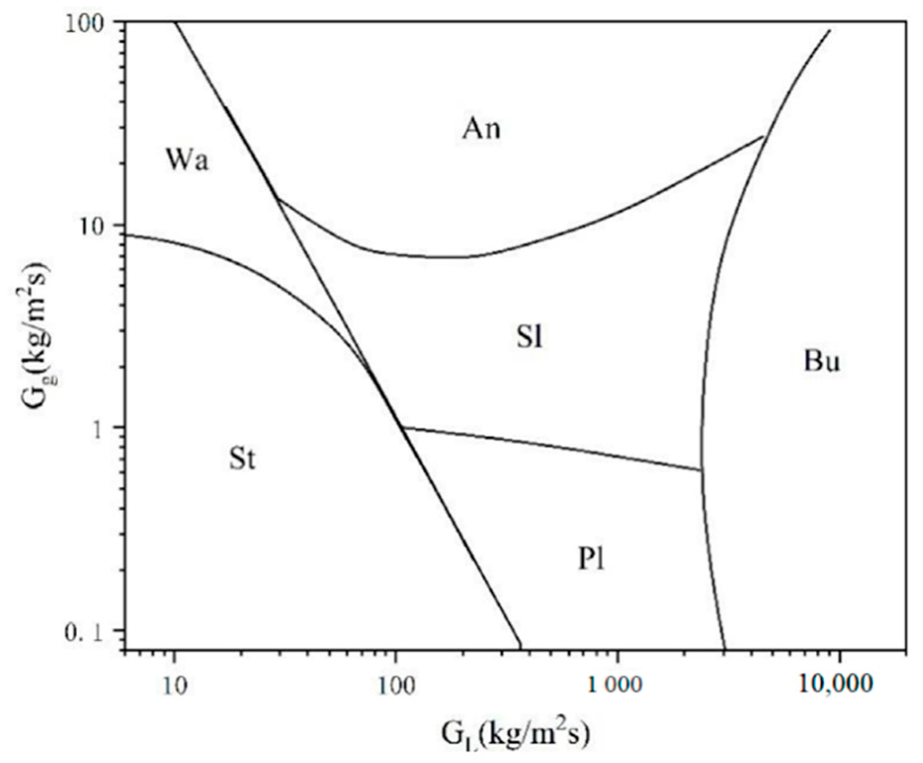
3.1. Flow Pattern for Straight Pipes

Figure 4 shows the volume fraction distribution of water phase under different gas superficial velocities and water content conditions inside the straight pipe. As shown, the fluid flow in the natural gas pipeline mainly depends on the gas superficial velocity and water content. When the gas superficial velocities are low, i.e., 0.5 m/s and 1 m/s, as shown in Figure 4a,b, respectively, the accumulation of the water phase at the bottom of the pipe is unaffected by the water content. When the gas superficial velocity is high, i.e., 3 m/s, as shown in Figure 4c, and the water content is low, i.e., 10%, the water phase gradually transforms from the aggregation state to a discrete state, and the water phase accumulation at the bottom gradually decreases. Under high water contents, i.e., 30% and 50%, although part of the water phase breaks away from the accumulation area at the bottom and is dispersed in the airflow, there are not many discrete water phases. Part of the water phase still accumulates at the bottom of the pipe. When the gas superficial velocity further increases, i.e., 5 m/s, as shown in Figure 4d, in the case of low water content, i.e., 10%, the accumulation effect of the water phase at the bottom completely disappears, and all the water phases have an accumulation state and are transformed into a discrete state. Even when the water content is high, i.e., 30% and 50%, the water phase accumulation at the bottom of the pipeline is no longer evident, and only a small amount of water phase accumulates at the bottom of the pipeline.

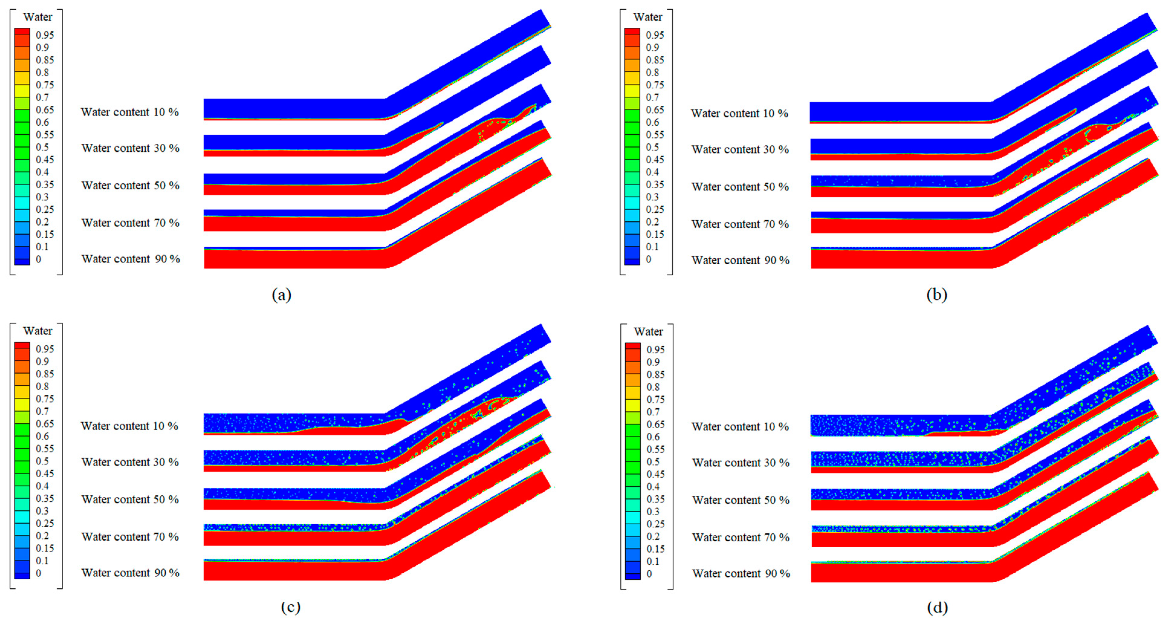
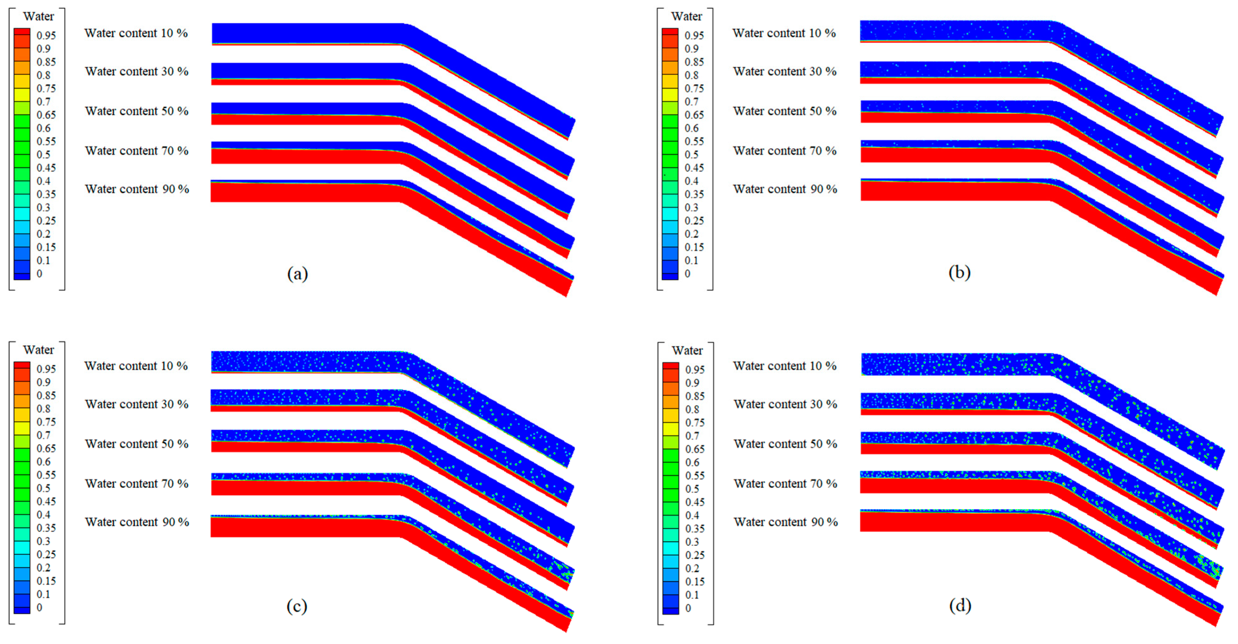
3.2. Flow Pattern for Inclined Pipe

3.2.1. Upward-Inclined Pipe

Figure 5 shows the volume fraction distribution of water phase under different gas superficial velocities and water content conditions in an upward-inclined pipe (30°). When the fluid superficial velocities are low, i.e., 0.5 m/s and 1 m/s, as shown in Figure 5a,b, respectively, the water phase in the fluid accumulates at the bottom of the pipe due to gravity, particularly at the elbow position. Even when the fluid contains only a small amount of water, i.e., 10%, water phase accumulation areas can be observed at the elbow of the pipe and in the straight region before the elbow. With the increase in the gas superficial velocity, i.e., 3 m/s, as shown in Figure 5c, the dispersion of the water phase in the pipe with a lower water content intensifies, i.e., 30%, and the water phase accumulation in the straight pipe section disappears after the elbow. The water phase tends to accumulate toward the elbow. However, when the water content is high, the water layer still occupies the bottom of the elbow, and there is no sign of dispersion or disappearance of accumulation. When the gas superficial velocity increases to 5 m/s, as shown in Figure 5d, the accumulation trend in the water phase at the elbow is already evident under a low water content observed previously. The dispersion effect of the bottom water phase in the straight pipe section before and after the elbow is also more severe. As before, this discrete phenomenon also did not appear under conditions of higher water content.

3.2.2. Downward-Inclined Pipe

Figure 6 shows the volume fraction distribution of water phase under different gas superficial velocities and water content conditions in a downward-inclined pipe (30°). The distribution law of the volume fraction of the water phase in the downward pipe is similar to the flow pattern of the straight pipe. Under the condition of low gas superficial velocities, i.e., 0.5 m/s and 1 m/s, as shown in Figure 6a,b, respectively, there is evident water accumulation at the bottom of the straight pipe section before and after the elbow. At this time, the water content has little effect on the water phase accumulation at the bottom of the pipe, which means that even if the water content is low at this time, i.e., 10%, the water phase will still accumulate at the bottom. This creates a severe corrosive environment. As the gas superficial velocity gradually increases, i.e., 3 m/s, as shown in Figure 6c, the water phase accumulation at the bottom of a pipeline with a low water content (i.e., 10% and 30%) gradually weakens, and the water phase in the aquifer gradually accumulates intermittently. In other words, under certain gas superficial velocity conditions, the water phase at the bottom of the pipeline with a low water content gradually changes from the accumulation state to the discrete state, and the pipeline corrosion phenomenon gradually weakens. However, in the case of high water content, i.e., 50%, 70%, and 90%, the high-velocity gas has a limited effect on the dispersion of the water phase at the bottom of the pipeline, and there will still be a large water accumulation area at the bottom of the pipeline. However, when the gas superficial velocity continues to increase, i.e., 5 m/s, as shown in Figure 6d, the water phase accumulation phenomenon in the pipeline with a low water content (i.e., 10% and 30%) is further weakened. At this time, the water phase in the pipeline is completely transformed from the accumulation state to the discrete state, and there is no longer any accumulation of the water phase at the bottom. In other words, the internal corrosion of the pipe walls can be alleviated.

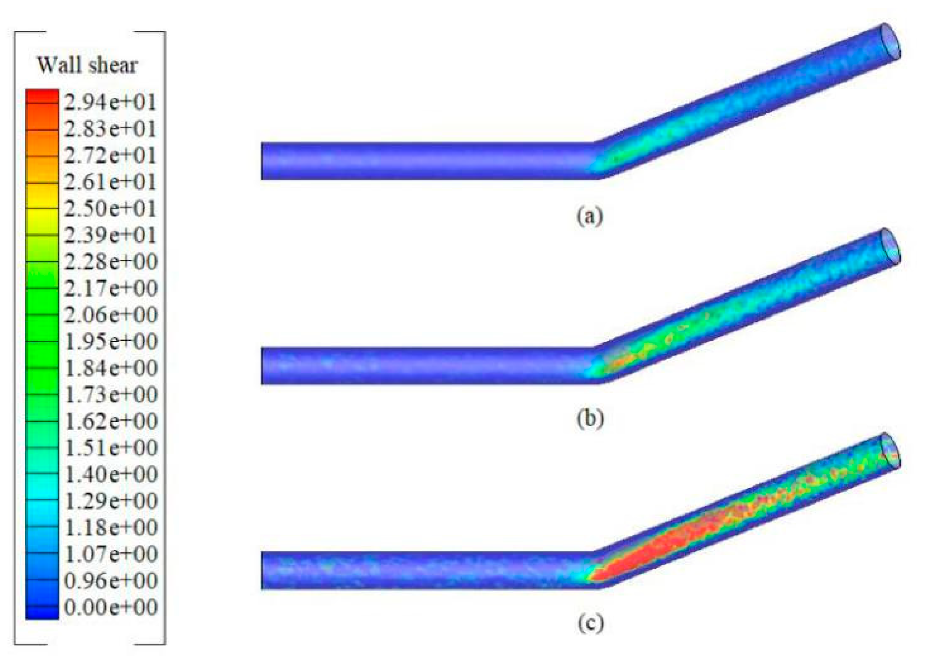
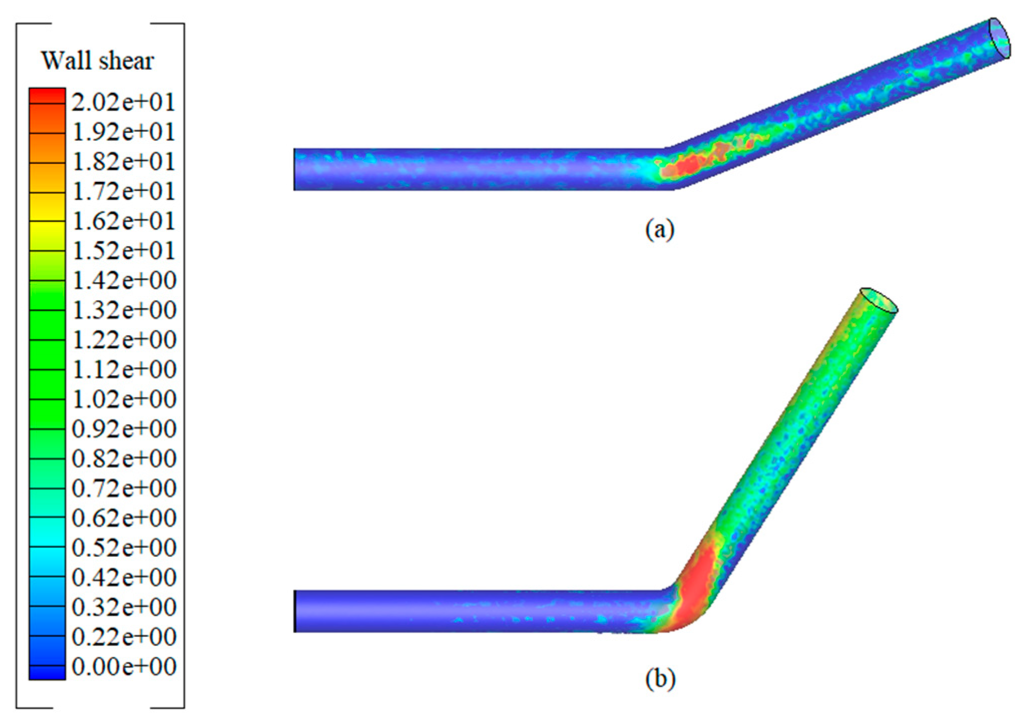
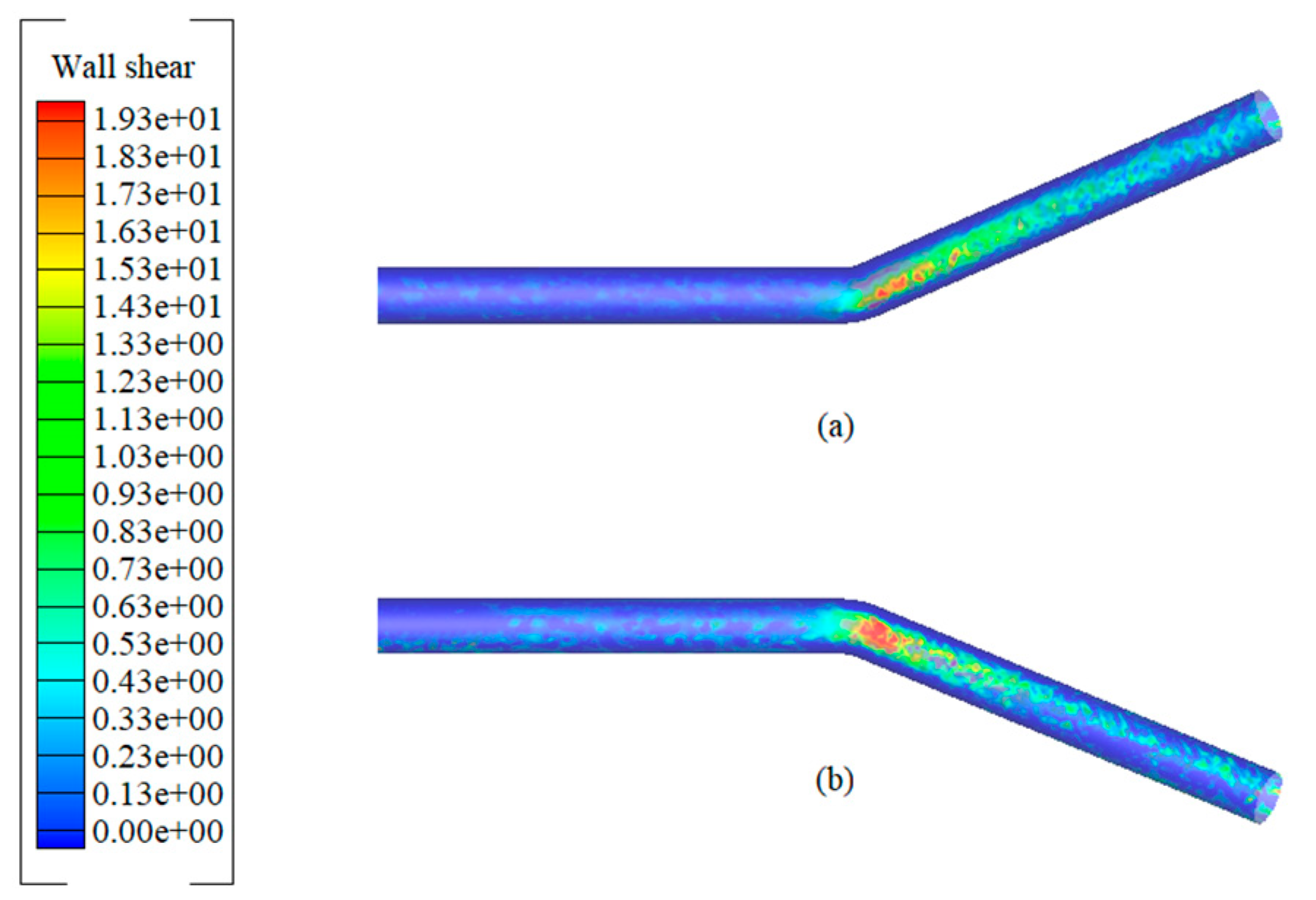
3.3. Wall Shear Stress in Inclined Pipes

In addition to the effect of fluid flow, in natural gas pipelines, the shear stress near the wall also has a great influence on the corrosion inside the pipeline. This is because the wall shear stress affects the formation and damage of corrosion products on the inner walls of the pipeline and even completely removes the formed corrosion product film [31].

Figure 7 shows the distribution of the wall shear stress at different gas superficial velocities in the upward-inclined pipe (30°) when the fluid contains 30% water and 70% gas. As the gas superficial velocity in the pipe increases, the maximum wall shear stress increases, and the wall shear stress is not uniformly distributed. In the upward-inclined pipe, the highest wall shear stress can be observed at the position of the elbow in the pipe. As the gas superficial velocity increases, the area where the maximum wall shear stress occurs also increases, and there is a tendency to extend upward.

Figure 8 shows the wall shear stress distribution at different water contents in the upward-inclined pipe (30°) when the gas superficial velocity is 5 m/s. With the gradual increase of the water content inside the pipeline, the concentration position of the shear stress near the wall remains basically unchanged, but the shear stress value changes more obviously. The location of the largest wall shear stress is always in the top area of the elbow and maintains a gradual upward trend.

Figure 9 shows the distribution of the wall shear stress at different inclined angles when the fluid contains 30% water–70% gas and the gas superficial velocity is 3 m/s. The wall shear stress gradually increases with the increase in the pipe inclination angle, and the distribution position of the wall shear stress has changed significantly. As the inclination angle of the pipe increases, the position where the maximum wall shear stress appears is more concentrated at the elbow, and the range of action is extended to the upper and lower walls of the elbow.

Figure 10 shows the distribution of the wall shear stress at different inclined directions when the pipe contains 30% water–70% gas and the gas superficial velocity is 1 m/s. The fluid flow direction in the upward-inclined pipeline is opposite to the direction of gravity, whereas the fluid flow direction in the downward-inclined pipeline is the same as the direction of gravity. Compared with the upward-inclined pipeline, the fluid in the downward-inclined pipeline slides forward a certain distance after it leaves the elbow because of the inertia of the water phase in the pipeline and the effect of gravity. This makes the position of the maximum wall shear stress of the downward-inclined pipe closer to the side wall surface than the upward-inclined elbow, which alleviates the corrosion effect at the elbow to a certain extent.

Through the above analysis, the wall shear stress distribution in the pipeline is uneven under different conditions, as shown in Figure 7, Figure 8, Figure 9 and Figure 10. For the upward-inclined pipe, the highest wall shear stresses are observed at the top and bottom of the elbow. For the downward-inclined pipe, the location of the maximum wall shear stress is delayed to a certain extent. As mentioned above, since the bottom of the upward-inclined pipe elbow is also the location of water accumulation, when corrosion occurs, a higher wall shear stress accelerates local corrosion, while this accelerated corrosion in the downward-inclined pipe is minor.

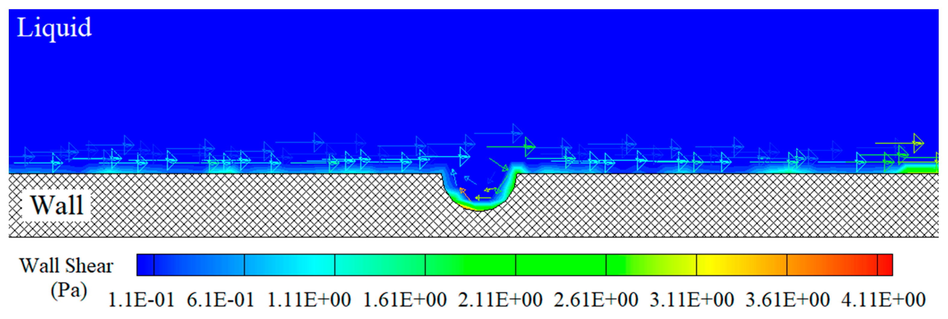
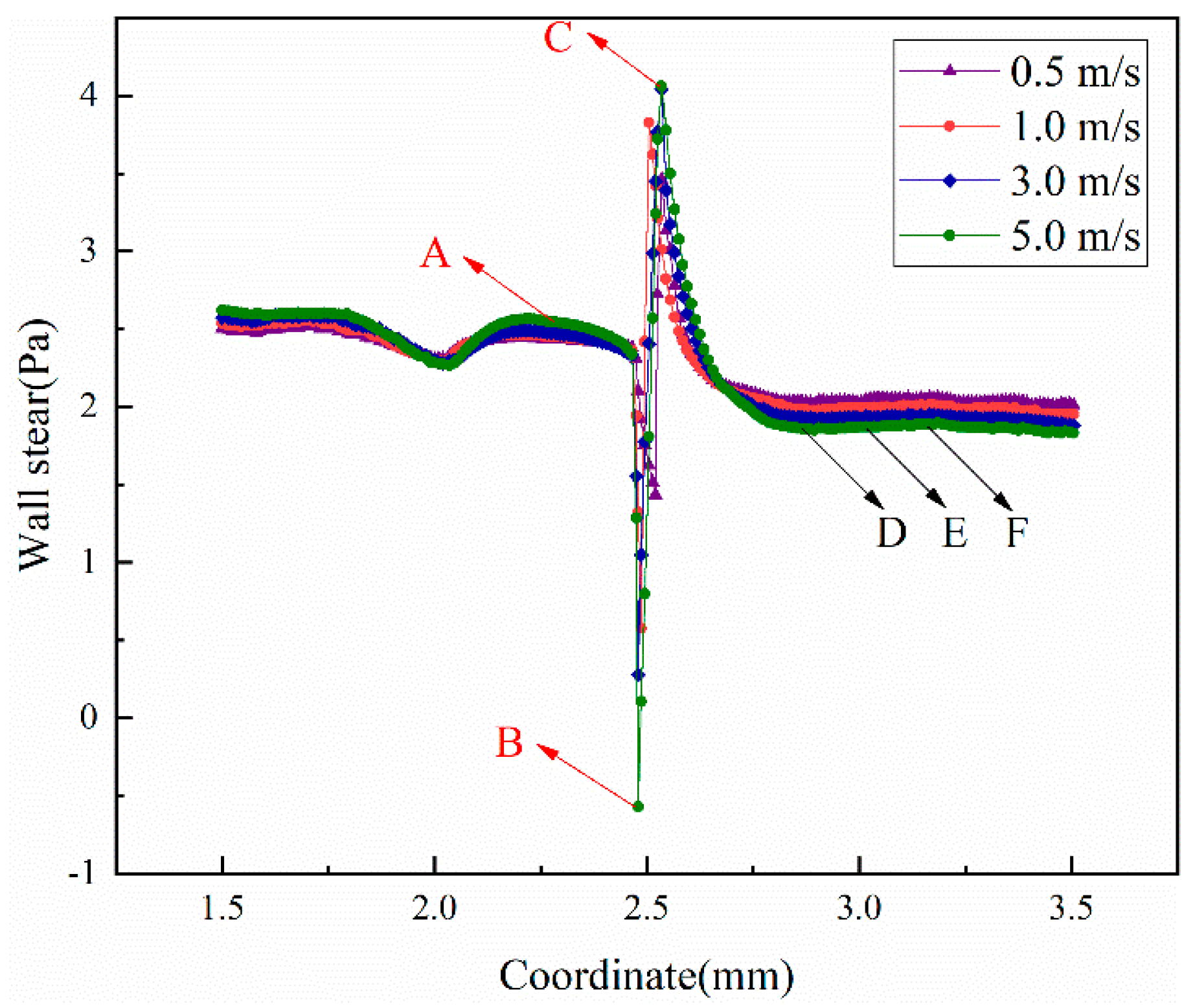
3.4. Localized Corrosion at Defect Sites

As mentioned above, the local water accumulation in the pipe is likely to cause local corrosion defects, and local corrosion is an important cause of leakage and perforation of the pipe. Therefore, it is necessary to simulate and analyze the flow field and wall shear stress at the defects. Figure 11 shows the corrosion defect model of the pipeline, where the diameter of the corrosion pit is 1.0 mm.

Figure 12 shows the flow field and wall shear stress distribution in the corrosion pit. The fluid flows in a ring shape at the corrosion pit, and the right-side wall in the pit is perpendicular to the fluid direction, which is mainly affected by the impact of the fluid. The left-side wall in the pit is parallel to the fluid flow direction and is mainly affected by the wall shear stress. Moreover, the wall shear stress on the left side of the pit is much greater than that on the right side; therefore, the damage of the corrosion product film on the left-side of the pit is more serious [18,23,32].

In addition, the wall shear stress not only causes the corrosion product film to fall off, but also accelerates the transmission speed of the medium in the fluid. High-pressure natural gas pipelines typically contain many bubbles in the water phase. When gas flows through the pits, because of the changes in the local pressure and wall shear stress, air bubbles tend to escape from the water phase and cause cavitation, which accelerates the local corrosion process. Figure 13 shows the change in the wall shear stress inside the pit. The changes in the wall shear stress under different gas superficial velocities are similar. With the increase in the gas superficial velocity, the wall shear stress at the upper and lower parts of the pipe decreases, the wall shear stress at the middle of the pipe increases, and the wall shear stress at the bottom of the pit is the highest.

4. Discussion

4.1. CO₂ Corrosion Mechanism

Based on the flow pattern classification made by Baker et al. [28], the flow pattern of the gas–liquid two-phase fluid in the pipeline is drawn, as shown in Figure 14. Here, ST is a stratified flow, Wa is a wavy flow, An is an annular flow, Sl is a slug flow, Pl is a plug flow, and Bu is a bubbly flow. The flow diagram is consistent with a previously published diagram [28].

When the gas superficial velocity in the pipe is low, the flow pattern in the straight, upward-inclined, and downward-inclined pipelines is stratified type. At this time, because of the high water content, the bottom of the pipe will be wetted by water, and the risk of fluid corrosion on the pipe wall is high. When the gas superficial velocity in the pipe is high and the water content is >30%, the flow patterns are wavy flow, annular flow, slug flow, plug flow, and bubbly flow. At this time, the water phase accumulates at the bottom of the pipe due to gravity and viscosity; therefore, the inside of the pipe is prone to corrosion. Only when the gas superficial velocity is high and the water content is low, water exists in the pipeline in a discrete form, and there is no accumulation of the water nor any internal corrosion.

The corrosion mechanism in a CO₂ gas environment is as follows:

Anode reaction:

Fe + 2e⁻ → Fe²⁺

(1)

Cathodic reaction:

H₂CO₃ + 2e⁻→ H₂ + CO₃²⁻

(2)

2H⁺ + 2e⁻ → H₂

(3)

When the concentration of Fe²⁺ and CO3²⁻ in the water exceeds a certain value, there is FeCO₃ precipitation that covers the metal surface to form a protective film [33,34]. The reaction process is as follows:

Fe²⁺ + CO₃²⁻ → FeCO₃

(4)

Based on the conclusions drawn by previous researchers, the formation of a complete corrosion film can effectively hinder the migration of ions and decelerate the corrosion reaction rate.

4.2. Localized Corrosion

From the above discussion, it can be found that the wall shear stress and bubble cavitation will destroy the corrosion product layer. In the fluid flow process, a wall shear stress is generated on the wall because of the effect of viscosity, which can be expressed by Equation (5):

$$\tau =\mu \frac{du}{dy}$$

(5)

where $\frac{du}{dy}$ is the velocity gradient in the y direction.

Figure 15 shows the cavitation process of the bubbles. As shown, the greater the gas superficial velocity, the greater the wall shear stress of the pipe. This phenomenon is not conducive to the formation of a complete corrosion product film in the pit, which makes the corrosion rate in the pit to be much higher than that at other locations and further accelerates the destruction process of the pit. At the same time, the wall shear stress accelerates the diffusion process of the bubbles in the liquid phase. Related studies have shown that the impact force due to bubble cavitation can be as high as 108 Pa [32]. There is no doubt that this magnitude of stress will affect the integrity of the product film and even directly damage the pipe matrix.

The above analysis shows that natural gas pipelines are often affected by the combined effect of electrochemical corrosion and fluid shock (mechanical behavior) due to the high gas superficial velocity. The wall shear stress at different parts of the pipeline is different; however, the wall shear stress at the water position of the pipe is often greater than that at other positions. An excessive local wall shear stress will cause bubble cavitation, which destroys the corrosion products on the pipe surface and the corrosion film that prevents corrosion. When the protective film of the layer formed by the corrosion product becomes thinner or even disappears, the fresh metal in the damaged part and the surrounding protected part form a local galvanic corrosion, which further accelerates the corrosion rate and leads to corrosion perforations [35,36]. Therefore, the FAC is the result of the combined effect of electrochemical corrosion and scouring, which has a greater effect than corrosion due to a single factor and is also greater than the combined effect of the two phenomena.

5. Conclusions

A multiphase flow simulation technology was used to study the gas–water distribution and wall shear stress of natural gas pipelines under different flow conditions. Based on the simulation results, the corrosion conditions of the pipeline were analyzed, and the effects of FAC on the damage of the pipeline corrosion product film and the local corrosion process were studied based on the results of the wall shear stress. The specific results of the study are as follows:

(1) The gas–water distribution in the natural gas pipeline was affected by both the water content and the gas superficial velocity. When the water content in the pipeline was low and the gas superficial velocity was high, the liquid in the pipeline was mostly distributed in the form of discrete phases, which means that no water could form. When the water content was high, there was consistent water accumulation at the bottom of the pipeline within the gas superficial velocity range under the actual working condition. Compared with straight pipes and downward-inclined pipes, water accumulation was more likely to occur in the upward-inclined pipes;

(2) In natural gas pipelines, the wall shear stress was significantly affected by the gas superficial velocity and the elbow angle of the pipeline and was less affected by the water content. The wall shear stress increased with the increase in the gas superficial velocity and the elbow angle, and the position of the maximum wall shear stress coincided with the water accumulation position in the pipe, both at the elbow and at the bottom of the inclined pipe;

(3) The electrochemical corrosion at the water accumulation position in the natural gas pipeline produced a corrosion product film that protected the metal matrix from further corrosion. However, under the action of the wall shear stress, local damage often occurred. The exposed metal due to the damage of the corrosion product film and the surrounding corrosion products formed a galvanic corrosion, which further aggravated the corrosion perforation phenomenon.

References

1. Sun, D.; Wu, M.; Xie, F. Effect of sulfate-reducing bacteria and cathodic potential on stress corrosion cracking of X70 steel in sea-mud simulated solution. Mater. Sci. Eng. A 2018, 721, 135–144. [Google Scholar] [CrossRef]
2. Gong, K.; Wu, M.; Liu, G. Stress corrosion cracking behavior of rusted X100 steel under the combined action of Cl and HSO3− in a wet-dry cycle environment. Corros. Sci. 2020, 165, 108382. [Google Scholar] [CrossRef]
3. Kahyarian, A.; Singer, M.; Nesic, S. Modeling of uniform CO2 corrosion of mild steel in gas transportation systems: A review. J. Nat. Gas Sci. Eng. 2016, 29, 530–549. [Google Scholar] [CrossRef]
4. Hu, H.; Cheng, Y.F. Modeling by computational fluid dynamics simulation of pipeline corrosion in CO2-containing oil-water two phase flow. J. Pet. Sci. Eng. 2016, 146, 134–141. [Google Scholar] [CrossRef]
5. Pouraria, H.; Seo, J.K.; Paik, J.K. A numerical study on water wetting associated with the internal corrosion of oil pipelines. Ocean Eng. 2016, 122, 105–117. [Google Scholar] [CrossRef]
6. Nesic, S.; Sun, W. Corrosion in Acid Gas Solutions. Shreir’s Corros. 2010, 2, 1270–1298. [Google Scholar]
7. Kahyarian, A.; Nesic, S. A new narrative for CO2 corrosion of mild steel. J. Electrochem. Soc. 2019, 166, C3048. [Google Scholar] [CrossRef]
8. Wang, Z.M.; Liu, A.Q.; Han, X.; Zhang, X.; Zhao, L.; Zhang, J.; Song, G.L. Fluid structure governing the corrosion behavior of mild steel in oil–water mixtures. Corros. Eng. Sci. Technol. 2020, 55, 241–252. [Google Scholar] [CrossRef]
9. Cheng, Y.; Bai, Y.; Li, Z.; Liu, J. The corrosion behavior of X65 steel in CO2/oil/water environment of gathering pipeline. Anti-Corros. Methods Mater. 2019, 66, 174–187. [Google Scholar] [CrossRef]
10. Murakami, S.; Mochida, A.; Ooka, R.; Kato, S.; Iizuka, S. Numerical prediction of flow around a building with various turbulence models: Comparison of k-ε EVM, ASM, DSM, and LES with wind tunnel tests. ASHRAE Trans. 1996, 102, 741–753. [Google Scholar]
11. Pantokratoras, I.; Arapatsakos, C. Turbulence models comparison for the numerical study of the air flow, an internal combustion engine. In Engineering Mechanics and Material; Wseas LLC: Santorini, Greece, 2014; pp. 178–184. [Google Scholar]
12. Charriere, B.; Decaix, J.; Goncalves, E. A comparative study of cavitation models in a Venturi flow. Eur. J. Mech.-B Fluids 2015, 49, 287–297. [Google Scholar] [CrossRef] [Green Version]
13. Kolev, N.I.; Kolev, N.I. Multiphase Flow Dynamics; Springer: Berlin/Heidelberg, Germany; New York, NY, USA, 2005; Volume 1003. [Google Scholar]
14. Balachandar, S.; Eaton, J.K. Turbulent dispersed multiphase flow. Annu. Rev. Fluid Mech. 2010, 42, 111–133. [Google Scholar] [CrossRef]
15. Xie, H.; Ren, H.; Li, H.; Tao, K. Quantitative analysis of hydroelastic characters for one segment of hull structure entering into water. Ocean Eng. 2019, 173, 469–490. [Google Scholar] [CrossRef]
16. Owen, J.; Ramsey, C.; Barker, R.; Neville, A. Erosion-corrosion interactions of X65 carbon steel in aqueous CO2 environments. Wear 2018, 414, 376–389. [Google Scholar] [CrossRef]
17. Malka, R.; Nešić, S.; Gulino, D.A. Erosion–corrosion and synergistic effects in disturbed liquid-particle flow. Wear 2007, 262, 791–799. [Google Scholar] [CrossRef] [Green Version]
18. Islam, M.A.; Farhat, Z.N. The synergistic effect between erosion and corrosion of API pipeline in CO2 and saline medium. Tribol. Int. 2013, 68, 26–34. [Google Scholar] [CrossRef]
19. Khan, R.; H Ya, H.; Pao, W. An experimental study on the erosion-corrosion performance of AISI 1018 carbon steel and AISI 304L stainless steel 90-degree elbow pipe. Metals 2019, 9, 1260. [Google Scholar] [CrossRef] [Green Version]
20. Pouraria, H.; Seo, J.K.; Paik, J.K. Numerical study of erosion in critical components of subsea pipeline: Tees vs. bends. Ships Offshore Struct. 2017, 12, 233–243. [Google Scholar] [CrossRef]
21. Zeng, L.; Zhang, G.A.; Guo, X.P. Erosion–corrosion at different locations of X65 carbon steel elbow. Corros. Sci. 2014, 85, 318–330. [Google Scholar] [CrossRef]
22. Wang, K.; Li, X.; Wang, Y.; He, R. Numerical investigation of the erosion behavior in elbows of petroleum pipelines. Powder Technol. 2017, 314, 490–499. [Google Scholar] [CrossRef]
23. Li, Y.; Li, J.; Wang, K.; Song, L.; Du, C.; He, R. The Effect of Flowing Velocity and Impact Angle on the Fluid-Accelerated Corrosion of X65 Pipeline Steel in a Wet Gas Environment Containing CO2. J. Mater. Eng. Perform. 2018, 27, 6636–6647. [Google Scholar] [CrossRef]
24. Lv, D.; Lian, Z.; Liang, L.; Zhang, Q.; Zhang, T. Study on Dynamic Erosion Behavior of 20# Steel of Natural Gas Gathering Pipeline. Adv. Mater. Sci. Eng. 2019, 1–15. [Google Scholar] [CrossRef] [Green Version]
25. Zhang, J.; Yi, H.; Huang, Z.; Du, J. Erosion mechanism and sensitivity parameter analysis of natural gas curved pipeline. J. Press. Vessel. Technol. 2019, 141, 034502. [Google Scholar] [CrossRef]
26. Wang, X.; Wang, X.; Wang, J.; Wang, G.; Pan, Y.; Yan, S. The Influence of O2 on the Corrosion Behavior of the X80 Steel in CO2 Environment. Int. J. Electrochem. Sci. 2020, 15, 889–898. [Google Scholar] [CrossRef]
27. Zeisel, H.; Durst, F. Computations of Erosion–Corrosion Processes in Separated Two-Phase Flows; NACE Corrosion: Houston, TX, USA, 1990. [Google Scholar]
28. Baker, O. Design of pipelines for the simultaneous flow of oil and gas. In Fall Meeting of the Petroleum Branch of AIME; Society of Petroleum Engineers: Dalla, TX, USA, 1953. [Google Scholar]
29. Desamala, A.B.; Dasamahapatra, A.K.; Mandal, T.K. Oil-water two-phase flow characteristics in horizontal pipeline—A comprehensive CFD study. Int. J. Chem. Mol. Nucl. Mater. Metall. Eng. World Acad. Sci. Eng. Technol. 2014, 8, 360–364. [Google Scholar]
30. Hancock, M.J.; Bush, J.W. Fluid pipes. J. Fluid Mech. 2002, 466, 285. [Google Scholar] [CrossRef]
31. Nesic, S. Key issues related to modelling of internal corrosion of oil and gas pipelines—A review. Corros. Sci. 2007, 49, 4308–4338. [Google Scholar] [CrossRef]
32. Li, W.; Pots, B.F.M.; Zhong, X.; Nesic, S. Inhibition of CO2 corrosion of mild steel—Study of mechanical effects of highly turbulent disturbed flow. Corros. Sci. 2017, 126, 208–226. [Google Scholar] [CrossRef]
33. Nesic, S.; Lee, K.L. A mechanistic model for carbon dioxide corrosion of mild steel in the presence of protective iron carbonate films—Part 3: Film growth model. Corrosion 2003, 59, 616–628. [Google Scholar] [CrossRef] [Green Version]
34. Nordsveen, M.; Nešic, S.; Nyborg, R.; Stangeland, A. A mechanistic model for carbon dioxide corrosion of mild steel in the presence of protective iron carbonate films—Part 1: Theory and verification. Corrosion 2003, 59, 443–456. [Google Scholar] [CrossRef] [Green Version]
35. Tan, Z.; Yang, L.; Zhang, D.; Wang, Z.; Cheng, F.; Zhang, M.; Jin, Y. Development mechanism of internal local corrosion of X80 pipeline steel. J. Mater. Sci. Technol. 2020, 49, 186–201. [Google Scholar] [CrossRef]
36. Tan, Z.; Yang, L.; Zhang, D.; Wang, Z.; Cheng, F.; Zhang, M.; Jin, Y. Development mechanism of local corrosion pit in X80 pipeline steel under flow conditions. Tribol. Int. 2020, 146, 106145. [Google Scholar] [CrossRef]
Figure 1. Physical model of a natural gas pipeline.
Energies 15 01694 g001
Figure 2. Meshing of the model used in the CFD simulation of an upward-inclined pipeline (30°).
Energies 15 01694 g002
Figure 3. Grid independence verification.
Energies 15 01694 g003
Figure 4. Distribution of the water phase inside a straight pipe with different gas superficial velocities, where (a) 0.5 m/s, (b) 1 m/s, (c) 3 m/s, and (d) 5 m/s.
Energies 15 01694 g004
Figure 5. Distribution of the water phase in an upward-inclined pipe (30°) with different gas superficial velocities, where (a) 0.5 m/s, (b) 1 m/s, (c) 3 m/s, and (d) 5 m/s.
Energies 15 01694 g005
Figure 6. Distribution of the water phase in a downward-inclined pipe (30°) with different gas superficial velocities, where (a) 0.5 m/s, (b) 1 m/s, (c) 3 m/s, and (d) 5 m/s.
Energies 15 01694 g006
Figure 7. Contours of the wall shear stress in an upward-inclined pipe (30°) carrying 30% water–70% gas at different gas superficial velocities, where (a) 1 m/s, (b) 3 m/s, and (c) 5 m/s.
Energies 15 01694 g007
Figure 8. Contours of the wall shear stress in an upward-inclined pipe (30°) with a gas superficial velocity of 5 m/s at different water contents, where (a) 10% water–90% gas, (b) 30% water–70% gas, and (c) 50% water–50% gas.
Energies 15 01694 g008
Figure 9. Contours of the wall shear stress at different inclined angles when the fluid contains 30% water–70% gas and the gas superficial velocity is 3 m/s, respectively: (a) 30° and (b) 60°.
Energies 15 01694 g009
Figure 10. Contours of the wall shear stress for both upward and downward pipes carrying 30% water–70% gas at a gas superficial velocity of 1 m/s (a) upward pipe, and (b) downward pipe.
Energies 15 01694 g010
Figure 11. Pipeline corrosion defect model.
Energies 15 01694 g011
Figure 12. Flow field distribution in the corrosion pit.
Energies 15 01694 g012
Figure 13. Wall shear stress along the flow direction.
Energies 15 01694 g013
Figure 14. Flow pattern diagram of gas–liquid two-phase fluid.
Energies 15 01694 g014
Figure 15. Schematic of bubble cavitation.
Energies 15 01694 g015