Surrogate Model of the Optimum Global Battery Pack Thermal Management System Control

Abstract

The control of the battery-thermal-management-system (BTMS) is key to prevent catastrophic events and to ensure long lifespans of the batteries. Nonetheless, to achieve a high-quality control of BTMS, several technical challenges must be faced: safe and homogeneous control in a multi element system with just one actuator, limited computational resources, and energy consumption restrictions. To address those challenges and restrictions, we propose a surrogate BTMS control model consisting of a classification machine-learning model that defines the optimum cooling-heating power of the actuator according to several temperature measurements. The la-belled-data required to build the control model is generated from a simulation environment that integrates model-predictive-control and linear optimization concepts. As a result, a controller that optimally controls the actuator with multi-input temperature signals in a multi-objective optimization problem is constructed. This paper benchmarks the response of the proposal using different classification machine-learning models and compares them with the responses of a state diagram controller and a PID controller. The results show that the proposed surrogate model has 35% less energy consumption than the evaluated state diagram, and 60% less energy consumption than a traditional PID controller, while dealing with multi-input and multi-objective systems.

1. Introduction

The world is undergoing a decarbonization mission and electromobility has a key role in that process [1]. The objective to 2050 is to reduce to zero, or almost zero, the use of internal-combustion-engine based vehicles in cities. In this context, electric vehicles are leading the market and have become the most interesting alternative to fuel engine-based vehicles [2]. Nonetheless, there are still some social aspects that need to be overcome to reach the defined objective, such as social anxiety concerning the safety and autonomy of electric vehicles [3]. In this regard, an optimum battery thermal management system (BTMS) is fundamental as it assures a safe operation of the batteries and has a direct influence on the autonomy [4].

A BTMS basically adjusts and balances the battery temperature to an appropriate range [5]. For that thermal management, BTMS-related technologies include BTMS design and BTMS online control strategies.

The BTMS designs aim to provide an adequate amount of heat dissipation or heat generation capability. The BTMS thermal properties are defined by the elements that integrate the whole thermal system. There are elements that can be implemented in the thermal system to increase the heat capabilities of the BTMS, such as heat pipes or phase change materials (PCMs) [6]. Nonetheless, most common BTMS designs employ only air or a liquid as the principal heat transmission element; the liquid based BTMS design is the predominant one in electric vehicles.

In any liquid BTMS design, there are five common elements: a pump, a chiller, a compressor, an evaporator, and a condenser [7]. There are other secondary elements that complement the whole BTMS, such as the expansion valve, thermocouples or pressure switches, but they do not have a relevant effect on the heat dissipation capability of the whole thermal system. However, they contribute to the control of the whole BTMS.

The BTMS control strategies aim to control the temperature range and distribution inside the battery pack [5]. These control strategies directly affect the reliability and efficiency of the overall thermal management of the battery [8]. There are many techniques available.

The proportional-integral-derivative (PID) control is widely used in industrial applications, and it is a suitable control algorithm to control the BTMS [9]. However, this kind of control is not able to deal with multi-input systems unless a complex decoupling process is provided [10], where the obtained control becomes sensitive to identification errors, to nonlinearities (strongly present in Li-ion batteries), and to the employed assumptions regarding the separability of the inputs. Besides, it shows deficiencies to balance temperatures and to minimize consumption. The PID is far from being an optimal control method for the BTMS [8]. A basic but also widely used control strategy is the state diagram control strategy (the on-off controller would be the simplest version of this type of controller) [11]. It is also called a macro-control or a rule-based control. The states are defined based on the observations of the real system and the controller will manage the actuators in consequence. A fuzzy controller would be a variant of these controllers, where fuzzy logic is added to the rule-based controller [12,13]. These kinds of controllers can control multi-input multi-objective (MIMO) systems, but they used to show high consumption rates and in some cases stability issues. Consequently, more intelligent and optimized control strategies have been researched. The model predictive control (MPC) [8,14] is an example. The model of the whole system is applied to predict the future behaviour and use this information to optimize the controller action. It is required to perform significant numbers of mid/long-term predictions in an optimization process context in every decision-making instant. The response of the controller is the optimum one and the safety is assured. Nonetheless, there are serious technical challenges to implement this kind of controller in a commercial BTMS. The actual limited computational resources lead to the need of applying significant simplifications on the model and on the optimization process [15,16]. It is still a challenge to develop a commercial MPC of a BTMS that uses a high-fidelity battery thermal model. Another intelligent controller is the machine learning based (or data-based) controller [17,18]. As a common tool, machine learning based controllers have a low computational cost. In addition, they are appropriate controllers to deal with MIMO systems [19]. Most of these kinds of studies focus on reinforcement type machine learning controllers. Nonetheless, the risks behind non-controlled batteries automatically preclude the use of reinforcement or iterative type learning processes on-board [17]. There are some exceptions, such as the controller developed by Kumar [20] using reinforcement learning. However, the leaning process required a baseline rule-based controller, which leads to obtaining a surrogate model of the baseline controller. The fact is that data-based control theory is still used by a minority in the industry due to the challenges it poses to the control engineers.

The industry is developing advanced BTMS designs that optimizes the heat transmission and the performance of the actuator [21]. As result, smaller thermal actuators provide the same performance rates as bigger actuators of conventional BTMS designs. However, in both cases, the total consumption depends strongly on the controller. The industry highly desires a BTMS controller that firstly, can operate safely; secondly, can deal with thermal inhomogeneities (deals with MIMO systems and does thermal balances); thirdly, optimizes the performance rate of the BTMS and reduces the total consumption (increasing like this the autonomy); and fourthly, has a low computational burden enabling it to be integrated in a commercial BTMS. There are many suitable controllers that provide acceptable responses, but as we have seen, none of them are able to fulfil these four control objectives.

This paper proposes a data-based control strategy that mixes the post-identification controller design with learning control aspects [19]. The proposed controller is a surrogate model (a black box model) that replaces the controller as a classic post-identification controller does. Nonetheless, the labelled data are obtained from trial-and-error simulations instead of real-life applications. Learning control concepts are brought to a simulation environment. Consequently, real life operation of the battery without an appropriate controller is avoided (possible catastrophic events of the system are avoided [22]); and a simple controller that provides optimum responses with a very low computational cost is constructed. As a result, the developed controller fulfils all four control objectives describe above in an optimal way.

The paper is structured in seven sections. In Section 2, the use case that contextualizes this study is presented: the evaluated battery pack and BTMS. In Section 3, the evaluated two traditional controllers are detailed. In Section 4, the development of the proposed controller is detailed. Firstly, how to get the labelled data required to train the surrogate control model is described in detail. Then, the evaluated machine learning algorithms are defined. In Section 5, the results are presented. Those results are discussed and compared in Section 6. Finally, the conclusions are presented in Section 7.

2. Use Case

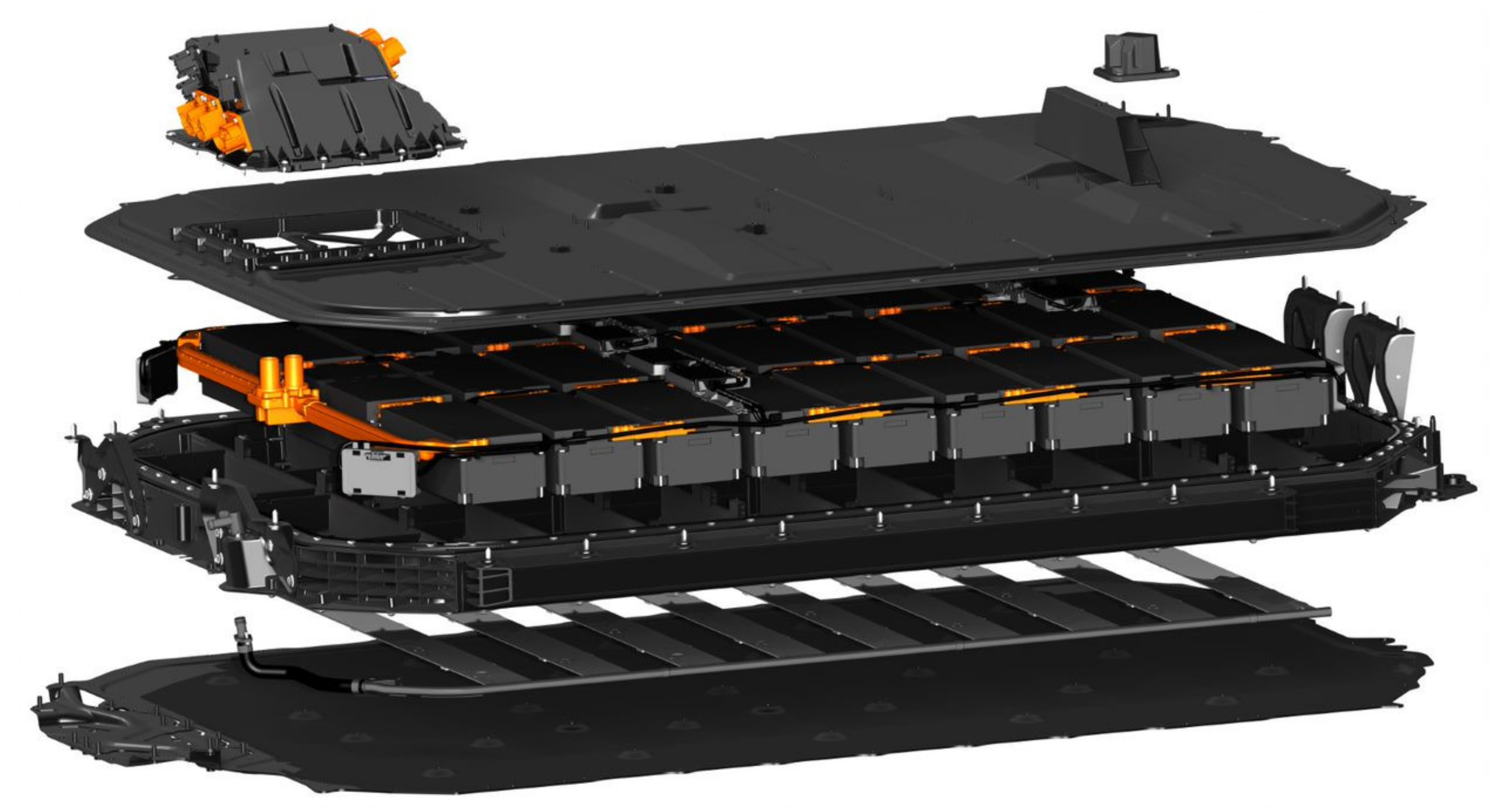
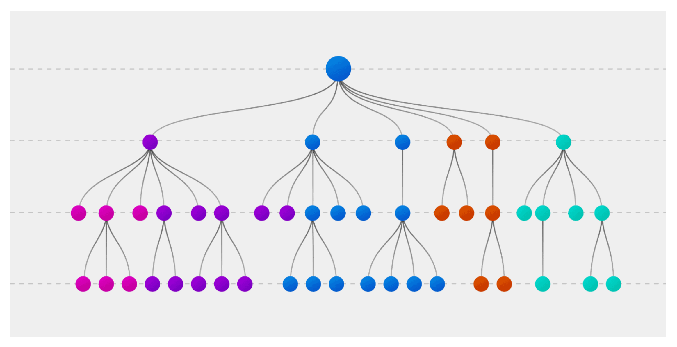
The proposed surrogate control model is applied to the BTMS of an electric light-duty vehicle with ultra-fast charge events (above 1C). The BTMS controls the temperature of each of the cells inside the battery pack. There are three different subsystem levels in the battery pack under evaluation: the cell, the module and the pack (see in Figure 1).

The basic unit of the battery is the cell. For this study, a commercial NMC-LTO prismatic cell of 23 Ah is selected. This type of cell is characterized for allowing fast and ultra-fast charges and for having a longer lifespan than an average NMC-graphite lithium-ion cell.

The next level is the battery module that is composed of 24 cells. The cells inside the module subsystem are electrically and thermally connected. Electrically speaking, it has two parallel branches of 12 cells in series. Thermally speaking, all 24 cells are assumed to be connected in parallel. It is expected that there will be temperature dispersion between the cells in the middle and in the centre. Nonetheless, the temperature difference between lateral and central cells has been minimized as the lateral ones have been isolated, and therefore, almost all the heat is directed to the cold plate. Besides, the control focuses on the critical cell of a module. The temperature dispersion of the cells inside the module is not observed. Consequently, it is assumed to be a perfect thermal parallelization of the cells.

The last level is the battery pack, which is composed of 27 modules (a total of 648 cells). Electrically speaking, it has three parallel branches of nine modules in series. Thermally speaking, it has nine parallel branches of three modules in series. It is assumed that the temperature at the beginning of each of the nine parallel branches is the same and that the modules that are connected in series have a domino effect on the heating of the cooling liquid (or cooling effect if the liquid is hotter).

The battery pack is thermally sensorized to measure the room temperature inside the battery pack, the cell temperature of each of the cells of the battery pack, and the liquid temperature inside the heat exchanger. The current and voltage at pack level are measured as well by the battery management system.

There is a unique actuator (a chiller) that heats up and cools down the liquid that goes though the heat exchanger circuit, which is in contact with the battery modules. The actuator, in the use case of study, can provide only six discrete cooling-heating power values, see

Table 1. Cooling-heating power options.

Level	Heat 2	Heat 1	Rest	Cool 1	Cool 2	Cool 3
Cooling power (W)	3000	1500	0	−666	−1333	−2000

.

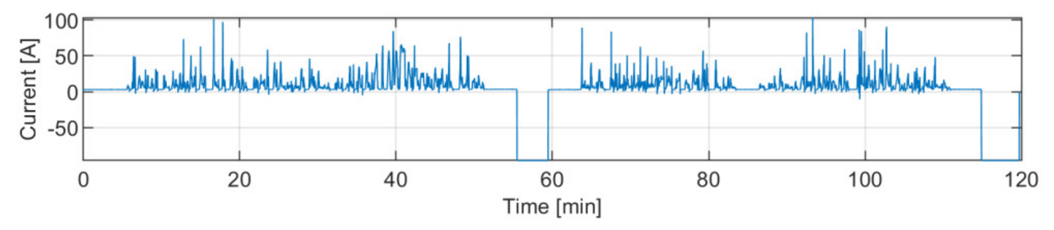
The most likely operation scenario for the electric light-duty vehicle under evaluation is defined. It is very likely to undertake the current profile shown in Figure 2 (it has two ultra-fast charge events) at a room temperature of 22 °C.

3. Traditional Controllers

Lithium-ion batteries have safety operating windows that must be respected. One of the most important safety operating windows is related with the temperature of the battery. The lithium-ion battery must be operated in a safe temperature range to avoid catastrophic events. This is the main reason why a thermal control is mandatory. For that aim, thermal controllers are implemented in the BTMS. Most of the controllers available in the industry are traditional controllers used on many other fields. The predominant controllers with more than a 95% are the state diagram controller and the PID controller [24].

3.1. State Diagram Controller

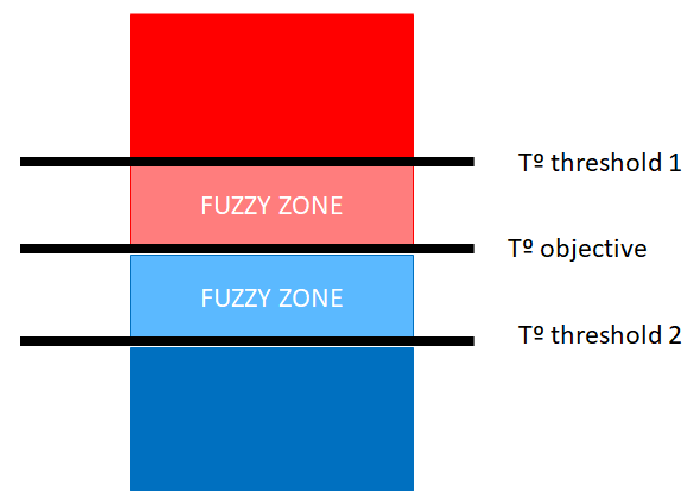
The state diagram controller is built with decision-making assessments associated with every state defined in the state diagram. The decision-making assessments basically are a set of control signals used to control the actuators. That set of values of those control signals are kept constant while the system remains in a specific state. When there is a change of the state, the set of values of those control signals will be changed accordingly to the change of state. The simplest state diagram controller is also called an on-off controller. The system of the on-off controller has two states, and the actuator receives two types of commands: switch on (100%) or switch off (0%).

In the use case study, a simple state diagram of two states was designed. The proposed controller is basically an on-off controller with a fuzzy zone. The controller tries to carry the controlled magnitude (the battery pack temperature) to the objective temperature. Nonetheless, unless the thresholds of the fuzzy zones are overcome, the controller does not act. Once one of the thresholds of the fuzzy zone is overcome, the controller acts until the temperature objective is reached. Afterwards, the controller is deactivated until once again a threshold of the fuzzy zone is overcome, see Figure 3.

3.2. PID Controller

The proportional-integral-derivative (PID) controller is the most common controller in the industry. This controller continuously calculates the error between the measured process variable and the desired setpoint in a closed loop feedback process. The calculated error is used to apply proportional corrections to the error (P), proportional integral corrections to the error (I) and proportional derivative corrections to the error (D) [25]. The transfer function of the PID controller is shown in Equation (1).

$$\mathrm{G}\left(\mathrm{s}\right)= \mathrm{P} + \mathrm{I} \times \frac{1}{\mathrm{s}}+ \mathrm{D} \times \mathrm{s},$$

(1)

In this study, the applied PID calculates the error between the mean temperature of a specific battery and the temperature setpoint of 25 °C. The response of the PID is sent to the BTMS to accomplish the heating and cooling actions required in each time instant.

The applied PID controller has been parametrized with the first presented Ziegler–Nichols method. This method consists of analysing the response of the system in a step form perturbation. The observed system behaviour is described with a first order transfer function, see Equation (2).

$$\mathrm{G}\left(\mathrm{s}\right)=\frac{\mathrm{K} \times { \mathrm{e}}^{-\mathrm{L} \times \mathrm{s}}}{\mathsf{\tau } \times \mathrm{s} +1},$$

(2)

The parameters obtained from the transfer function of the system are used to infer the parameters of the PID, as shown in

Table 2. Ziegler–Nichols method; theory and estimations.

Parameters	Theory	Estimations
P	$1.2\times \frac{\mathsf{\tau }}{\mathrm{K} \times \mathrm{L}}$	25.18
I	$\mathrm{P} \times \frac{1}{2\times \mathrm{L}}$	1.1448
D	$\mathrm{P} \times 0.5\times \mathrm{L}$	138.52

.

Finally, we mention that the applied PID has the saturation values of −1 and 1 for the whole PID and for the integral error, as this last saturation is crucial to prevent “wind up” effects of the proportional integral control element.

4. Proposed Control Model

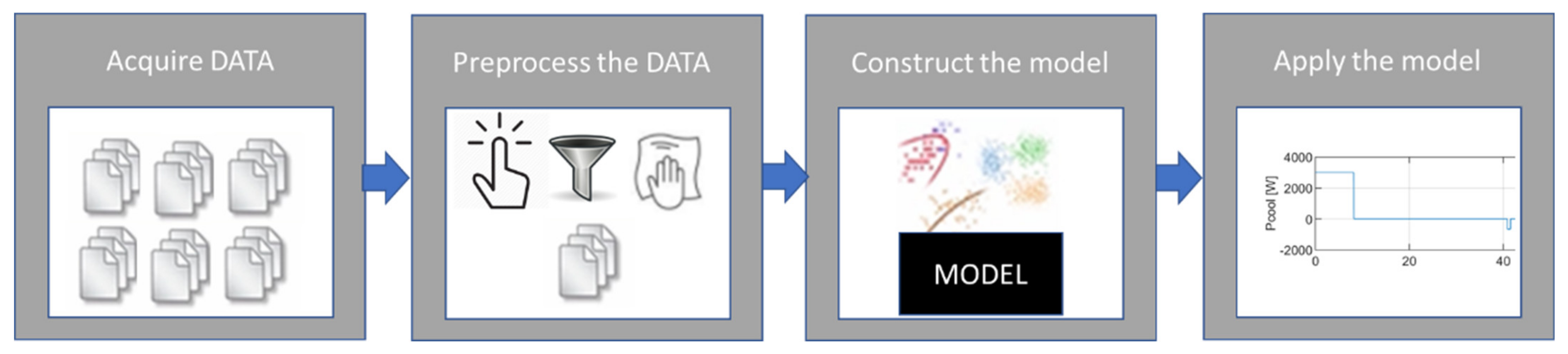
This paper proposes a surrogate control model that firstly, can operate safely; secondly, can deal with thermal inhomogeneities (deals with MIMO systems and does thermal balances); thirdly, optimizes the performance rate of the BTMS and reduces the total consumption (increasing like this the autonomy); and fourthly, has a low computational burden to enable its integration in commercial BTMS. The flow chart that describes the construction process of this surrogate model is shown in Figure 4.

This paper proposes to generate the surrogate model using machine learning algorithms. Machine learning algorithms find patterns in massive amounts of data. The algorithms can focus on identifying and grouping data sets based on their characteristics (unsupervised learning), or they can focus on modelling certain process by undergoing a training, where the inputs and outputs of the model are defined (supervised learning). The objective of this paper was to obtain a BTMS control algorithm. In other words, our objective was to model a certain process: the control itself. Therefore, supervised learning algorithms were selected and evaluated. As a result, a black-box model that surrogates the functions of an actual controller was developed.

Nowadays, the implementation of any machine learning algorithm is trivial as there are robust libraries that contain those algorithms, as well as generic training tools for them (see Figure 5). For this paper, the MATHWORKS’ machine learning library named “statistics and machine learning toolbox” was used. Nonetheless, the data acquisition task and the data pre-processing task required to generate the machine learning algorithm (clean the data, select the relevant data, adjust the data to the available training tools, etc.) was completely data dependent. Each machine learning project has different data acquisition and pre-processing needs. There is not any generic data structure. Therefore, these two tasks almost require 99% of the invested effort in developing the machine learning algorithm. This project was not different to others and most of the effort was spent in the acquisition and pre-processing of that labelled data.

Additionally, it is important to understand that the performance rate of the final algorithm (our controller) depends strongly on the quality of those labelled data more than the actual algorithm itself. The model is as good as the available data in the training process. This fact supports even more the desirability of investing the main effort in data acquisition and pre-processing tasks.

For this machine learning project, the acquisition of the labelled data was especially challenging. The acquisition of labelled data required us to define the response that the model had to make in each decision-making event. This decision-making can be guessed by running an actual controller. Nonetheless, the obtainable surrogate model from the labelled data of a traditional controller was not much use because it will always have a lower performance than the one it is surrogating; the surrogate model does not give any additional value.

Instead, this paper proposes a methodology to determine the optimum response of the actuator regardless of its on-board applicability; we focus on getting the labels (the real aim). The proposed labelling process is the simplest but most robust way of doing it: to test all the possibilities and choose the optimum one. For that, a simulation environment of the system was built where the optimum response was selected thanks to a linear programming (LP) optimization algorithm (a trivial task once the results of all the simulations are available). As a result, artificial labelled data that contained global optimum responses in a wide spectrum of battery states was generated.

The states of the system were described by different properties. Those which affected the most the thermal management were selected.

The response of the proposed surrogate control model (the decision-making assessment) is the discrete value of the heating-cooling power that the actuator of the BTMS must provide to the battery pack, see Table 1. The developed controller with the artificially generated labelled data gives globally optimum responses in heterogeneous operating conditions and in any likely battery state. It allows a safe operation while minimizing the consumption of a MIMO system. Moreover, its implementation in any commercial BTMS is possible because it has almost zero computational cost.

4.1. Supervised Learning Algorithms

A supervised learning algorithm analyses the training data and produces an inferred function. This function can describe the training data. If properly trained, the inferred function can correctly determine the class labels for unseen instances (or states).

Supervised learning algorithms can be classified into two type of modelling algorithm: classification and regression. In general, classification algorithms are applied in image processing applications, while regression algorithms are applied in existing system’s modelling applications. Nonetheless, both can be used in both type of applications, and the feature that differentiates them the most is the features of the output. If the output is discrete, a classification algorithm would be more appropriate than a regression algorithm; and if the output is continuous, the regression would be more appropriate. In this case, the output of the control algorithm is discrete (there are only six options), therefore, the selected type of machine learning algorithm was a classification supervised learning algorithm.

Among the available classification supervised learning algorithms, the most common ones are the decision tree, the k-nearest neighbour, the naive bayes and the support vector machine (SVM).

4.1.1. Decision Tree

A decision tree is one of the simplest algorithms that could be used in a classification project. The features of the samples forming the data are analysed. Based on those features, the samples are classified (split). The training process of this algorithm consists of classifying the labelled data. The result of this training process is a model constructed with a bunch of questions with answers. When applying it to a new sample, the model goes through the whole tree to reach the leaf that labels the evaluated sample [26], see structure in Figure 6.

4.1.2. K-Nearest Neighbour

K-nearest neighbour algorithm classifies new samples based on the similarities of the samples. The labelled data on the training is used to develop a fictitious neighbourhood of samples (a table). New samples are compared with the ones that already are in the neighbourhood. Then, the label of the sample that shares more similarities with the new sample is used to label this new sample. It shares many similitudes with a look up table function.

4.1.3. Naive Bayes

Naïve Bayes is an algorithm to construct a classifier using N different features or labels that are independent from each other. This supervised algorithm, calculates the probability of each feature from a training dataset. This probability calculation varies from one dataset to another, in some cases a normal distribution can be used to calculate those values, but in some other cases, a binomial distribution might make more sense. This calculation is directly linked to the domain of the problem. Once the probability of each feature is calculated and the probability of the classification outcome is known, based on the training data, the feature probabilities are combined against the total probability for each outcome, and the outcome resulting in the highest value is the classification result.

4.1.4. Support Vector Machine

SVM algorithm is a kernel-based method that belong to a family of generalized linear classifiers [27]. The SVM comes from the nonlinear generalization of the Generalized Portrait algorithm developed by Vapnik et al. in the 1960s. It projects the original low dimension data space to high dimension feature space. This projection is equivalent to transforming non-linear problems in a lower dimension to linear problems in higher dimensions. The SVM fits the sample data in the higher dimensional feature space by the optimization of the margin using a linear function [28]. In this study, the gaussian kernel is selected to construct the classification SVM algorithm.

4.2. Labelled Data

The so-called labelled data contains samples that have been tagged with labels. In the context of this study, the samples are the group of properties that defines a specific state or operating condition of the battery pack (room temperature, liquid temperature, cell temperature and heat generation) and the labels are the response of the BTMS at that specific state.

The labelled data are the most crucial element in a supervised learning algorithm. The final product (our surrogate model) will be as good as the applied labelled data to train the algorithm. The performance of the constructed classification algorithm will be equal to the quality of that labelled data. The scarcity of samples or inaccuracy in the labelling will lead to an imprecise model.

These data can be obtained from field data (on-board measurements) or from simulations (artificially generated data). In this case, field data were not available nor interesting, so the data was artificially generated by simulations. Firstly, a vast number of samples that cover all observable states was defined; and secondly, each of the defined samples was labelled thanks to the designed labelling algorithm.

4.2.1. Samples

Each of the samples of the labelled data represents a specific state of the battery (likely to be observed). These states were defined by different features. There are many features that could describe a state of a battery. For example, the most common way of describing the state of a battery is by the amount of storage energy, which is also called state of charge (SOC). Nonetheless, the features of interest to construct the samples in this study were the ones that had the highest effect on the thermal management of the battery pack. The samples will be used to construct a model that relates the features of those states with the required BTMS decision-making assessment. Therefore, the selected features and the thermal behaviour of the battery needed to be correlated; of all possible features, we have cherry-picked the ones shown in

Table 3. Cherry-picked inputs of the controller.

Parameter	Description
Troom	The room temperature (inside the battery pack).
Tcellxx	All the battery temperatures, where xx is the cell number inside the battery pack.
Tlq	The BTMS liquid temperature (the temperature at the return point of the actuator of the BTMS).
Qbat	The heat generation of the battery system (the total heat generation of the whole battery pack).

.

Once the features that compose a sample have been selected, a bunch of samples that cover all possibilities on the use case need to be generated. For this purpose, those samples must account for the operating limits imposed in the use case under evaluation. In addition to this, those samples need to be representative of the samples that will be available when applying the control on-board. Based on these two criteria, the value range and the characteristics of the features that compose the samples were specified.

The room temperature is measured continuously. Most likely, the room temperature will be 22 °C. It is also expected not to suffer huge changes. Therefore, samples with instant values of 22 ± 5 °C should cover all possibilities.

Every cell temperature is measured continuously. In this use case, the selected battery can only work between a safe operating thermal window of 5 °C to 48 °C. It is expected to perform a proficient thermal management, hence, the individual cell temperature is expected to be between 15 °C and 35 °C. Therefore, the samples with unitary instant values between 15 °C and 35 °C should cover all possibilities. However, there is more than one cell temperature measurement. It is not expected that there will be thermal inhomogeneities inside a module sub-system. The cells are all attached. They heat-cool each other, achieving a passive thermal balancing. Nevertheless, it is expected that there will be thermal inhomogeneities between modules of the same cooling-heating line inside the battery pack. The inhomogeneities are not expected to be higher than 2 °C, but one of the aims of the proposal controller is to deal with these inhomogeneities. Therefore, all kinds of thermal inhomogeneities in a specific cooling-heating line (always inside the expected range from 15 °C to 35 °C within the maximum observable inhomogeneity of 2 °C) were considered when generating the samples.

The liquid temperature of the actuator is measured continuously as well. It is expected to be equal or below the individual cell temperature. Therefore, the maximum temperature the liquid will take is 35 °C. The minimum temperature of the liquid depends on the cooling capabilities of the actuator and the BTMS efficiency. In our case study, the expected minimum liquid temperature was 5 °C.

The heat generation of the battery system is not measured. Instead, the heat generation is estimated from the continuously measured current and the continuously estimated open circuit voltage (OCV) and impedance (estimated by the BMS), see Equation (3) [29]. The values given to this feature were dependent to the most likely current profile (already defined in Section 2), and the OCV and impedance of the battery when going through that current profile. In consequence, the values given to this feature were not defined at the beginning, but rather were continuously estimated on the labelling process.

$$Q_{bat}\left(t_k\right) = I{\left(t_k\right)}^2 \times R + I\left(t_k\right) \times T_{bat}\left(t_{k - 1}\right) \times \frac{dOCV}{dT},$$

(3)

In an ideal word, the controller would act according to future heat generation estimations. However, the evaluated BTMS will not be able to predict the future heat generation. Consequently, only current and past estimations were available to fill the samples. In this context, we were forced to assume that the future heat generation will be the same as the already observed one. The controller will act based on the observed heat generation instead of the predicted one.

In addition to all this, the stability of the future controller must be considered. For that, the effect the selected features have on the controlled feature (the cell temperature) were evaluated:

• The cell temperatures used in each sample were the feedback for the controlled feature itself.
• The room and liquid temperatures were the same type of feature as the controlled one. They shared the same dynamics.
• The heat generation shows faster changes than the controlled one (it shares the same dynamics as the current, see Figure 2) and has a cumulative effect on cell temperature (the temperature changes only when heat is applied in a period of time).

Consequently, the update rate of each of the cell temperature, the room temperature and the liquid temperature must be in concordance with the decision-making frequency; unitary values of these features are continuously updated. On the other hand, rather than the use of unitary heat generation estimations, the samples were constructed with the mean value of the heat generation during a specific period of time: 100 s. This period was empirically set up to reduce the dynamics of the heat generation but to be representative enough to the undergone changes in a short/mid-term.

4.2.2. Labels

The samples were labelled with global optimum decision-making assessments. Each battery state was labelled with the cooling-heating power that the actuator of the BTMS had to deliver to the battery pack. Therefore, the labels were the cooling-heating power values. The cooling-heating power values used as labels were the global optimum solutions of the samples. Nonetheless, there was not an easy way of determine those labels. If it were easy, it would not be necessary to develop complex controllers in the first place. This was the reason why this study provides a methodology to perform the global optimum labelling of each of the samples, see pseudo-code in Algorithm 1.

Algorithm 1. Pseudo-code of the labelling process.

${\left\{Labe{l}^{\left(i\right)}\right\}}_{i=1}^{NxM}=Labelling\left({\left\{va{r}_{sample}{}^{\left(j\right)}\right\}}_{j=1}^P,{\left\{ou{t}_{options}{}^{\left(k\right)}\right\}}_{k=1}^Q,{\left\{o{p}_{criteria}{}^{\left(u\right)}\right\}}_{u=1}^L,t_{int},t_{sim}\right)$

1:    ${\left\{{\vartheta }_{IN}^{\left(i\right)}\right\}}_{i=1}^M=GRID\left(va{r}_{sample}{}^{\left(1\right)},\cdots ,va{r}_{sample}{}^{\left(P\right)}\right)$

2:    ${\left\{{\vartheta }_{OUT}^{\left(j\right)}\right\}}_{j=1}^R=GRID\left(ou{t}_{options}{}^{\left(1\right)},\cdots ,ou{t}_{options}{}^{\left(Q\right)},t_{int},t_{sim}\right)$

3:    for $i=1$ to $M$ do

4:       for $j=1$ to $R$ do

5:          ${\left\{va{r}_{sim}{}_j^{\left(k\right)}\right\}}_{k=1}^S=BATT\_MODEL\left({\vartheta }_{IN}^{\left(i\right)},{\vartheta }_{OUT}^{\left(j\right)},t_{sim}\right)$

6:       end for

7:       ${\left\{Labe{l}_i^{\left(l\right)}\right\}}_{l=1}^N=LINEAR\_PROGRAMMING\left({\left\{{\left\{va{r}_{sim}{}^{\left(j\right)\left(k\right)}\right\}}_{k=1}^S\right\}}_{j=1}^R,{\left\{o{p}_{criteria}{}^{\left(u\right)}\right\}}_{u=1}^L,t_{int}\right)$

8:    end for

Where:

$N$ = Number of samples obtained from a single linear programming optimization exercise;

$M$ = Dimension of the sample grid and number of samples to be analysed;

$P$ = Number of variables that forms a sample;

$Q$ = Number of discrete values of the controlled variable;

$L$ = Number of optimization criteria;

$R$ = Number of decision-making combinations for the evaluated sample;

$S$ = Number of variables recorded for the linear programming;

${\vartheta }_{IN}^{\left(i\right)}$ = ( $i$)th evaluated combination of the input variables of controller, ($i$)th sample;

${\vartheta }_{OUT}^{\left(j\right)}$ = ( $j$)th evaluated profile of the controlled variable for the whole $t_{sim}$;

$Labe{l}_i^{\left(l\right)}$ = $\left(l\right)$th Label of the ($i$)th sample;

$va{r}_{sample}{}^{\left(j\right)}$ = Value vector of ( $j$) Health Indicator;

$ou{t}_{options}{}^{\left(k\right)}$ = $\left(k\right)$th discrete value that the output variable can take;

$o{p}_{criteria}{}^{\left(u\right)}$ = ($u$)th optimization criterion;

$t_{int}$ = Time interval that the controlled variable is kept constant in the simulation;

$t_{sim}$ = Simulation time. It represents the length of the current profile (a sample variable);

$GRID$ = Generator of the evaluated numerical grid;

$BATT\_MODEL$ = Battery electric-thermal model of the battery pack;

$LINEAR\_PROGRAMMING$ = Number of His;

$va{r}_{sim}{}_j^{\left(k\right)}$ = $\left(k\right)$ th recorded simulation variable of the $j$ th evaluated output profile.

The proposed methodology to find those global optimum labels was inspired in iterative learning [19]. It consisted of simulating all the control possibilities and performing a LP optimization. As simple as that. The simulation of all the possibilities allowed us to perform a LP optimization in an easy way. Besides, global optimum values were obtained as all possibilities were considered. The concept behind the methodology was quite simple. The implementation of it, not so much.

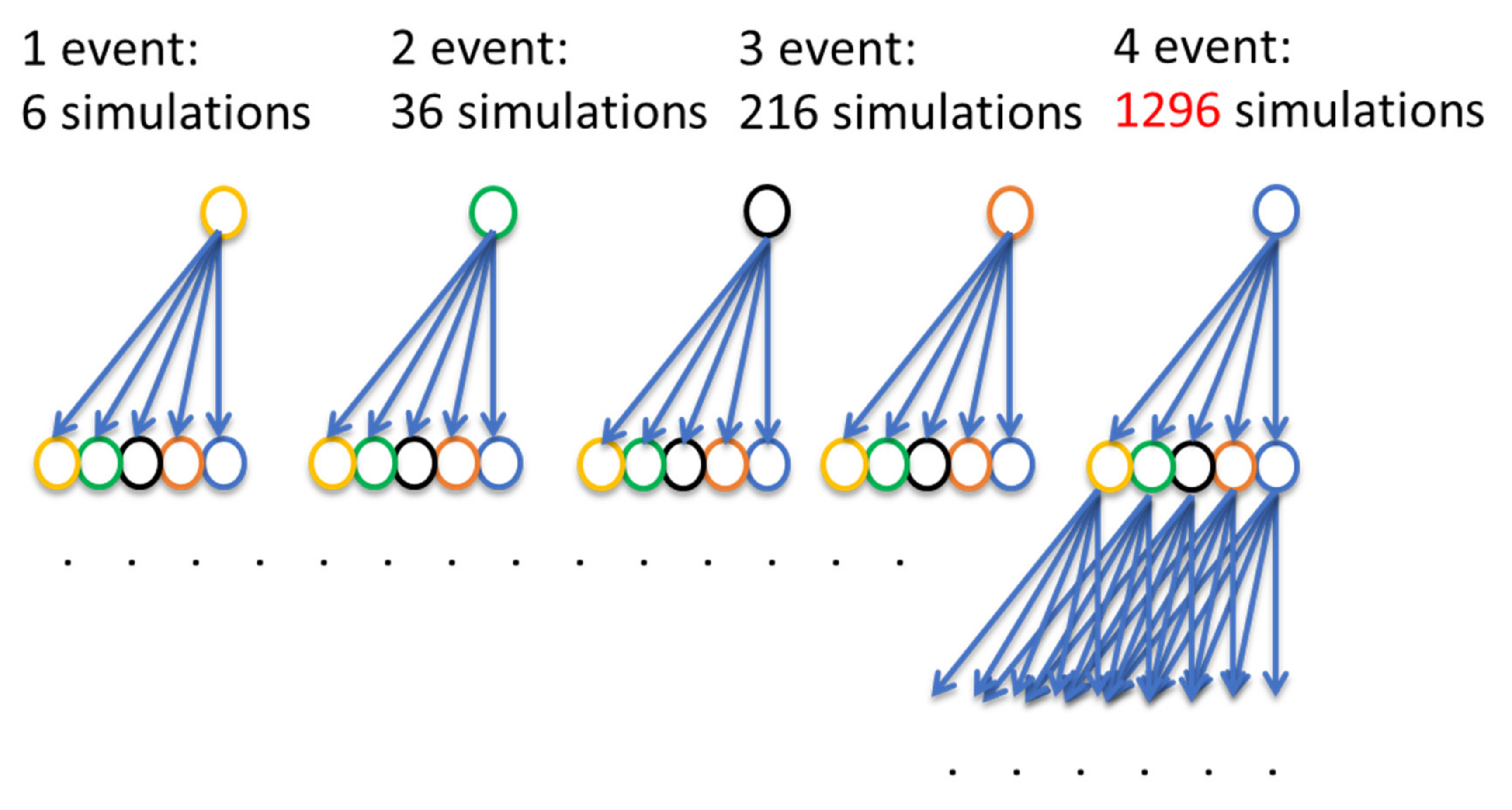
Firstly, all the control possibilities must be simulated for each of the samples. The number of simulations depends on the discrete values of the label, and the number of decision-making assessments done in a simulation. The number of control possibilities were always six (see Table 1) in every decision-making assessment. Nonetheless, the linear increase of decision-making events rises exponentially with the number of total simulations, see Figure 7. Subsequently, the simulations were set up to minimize the decision-making events that were undergone in each simulation.

Secondly, the decision-making frequency had to be established. The decision-making frequency applied on the simulation will determine how many decision-making events will be done in a specific simulation period. It was desired to have a decision-making assessment each time the temperature was measured. Nonetheless, the number of simulations grows exponentially with the linear growth of the number of decision-making events, see Figure 7.

Thirdly, the implementation of the LP involves specific optimization criteria. In this study, three different optimization criteria were designed:

• Thermal satisfactory operation (accurate control).
• Thermal homogeneity of the batteries (balancing capability).
• Energy efficiency (reduction of the consumption of the BTMS).

These optimization criteria were translated into a LP equation system and applied to get the optimized label for each sample. This LP equation compared the total mean error of all the cells, the maximum variance between cells and the total consumption of the BTMS in terms of cooling-heating power. Among these three comparisons, the last one, that which compared the total consumption, required us to simulate the longest possible current profile. The longer the current profile is, the more relevant the calculated total consumption will be and the better the final controller will be. Nonetheless, the length of the current profile had an exponential relationship with the number of simulations required to get all control possibilities. Long current profiles implicitly demand higher numbers of decision-making events. As seen in Figure 7, the linear increase in decision-making events increases exponentially with the number of simulations.

The implementation of the methodology puts into perspective the length of the simulated current profile, the decision-making frequency, and the number of required simulations to do so. The maximum number of decision-making events was set to four (due to computational resources), leading to a total of 1296 simulations to label one sample.

On the other hand, it was desired to have frequent decision-making events in long current profiles. These are contradictory requirements. Long current profiles with four decision-making events leads to infrequent decision-making events. Simulations containing four decision-making events with short time intervals between them forces the shortening of the length of the current profile. The interval between decision-making events was set by considering two aspects. Firstly, this interval had to be frequent. It cannot be long. Secondly, the interval must have a minimum length. The cooling-heating power had to be kept at a constant a minimum length of time to affect the controlled feature: the battery pack temperature. Based on this, the interval between decision-making events was set to 150 s. This means that the length of the simulated current profile was set to 10 min.

The interval between decision-making events was considered acceptable as the controlled feature (the battery pack temperature) was expected to show observable changes in this period of time. The length of the current profile, in contrast, is not long enough to properly address the consumption optimization criterion, at least as one labelled sample. However, if all the labelled data were considered as one, these labelled data can be interpretated as an ensemble learning process [30]. Small and simple models that describe partly a truth can be ensembled to create a complex model that describe the whole truth. Each of the labelled datasets are like small simple models that can describe partly the whole current profile. The constructed final model with those labelled data (those small models) will give optimum responses in the whole window of the current profile. Besides, going further with this assembling concept, it was possible to consider as suitable labelled datasets each of the four decision-making assessments done in each 10 min current profile. As a result, four datasets could be saved in each simulated sample. This multiplies by four the number of labelled datasets that will be obtained at the end of the whole labelling process.

The simulations resort to a 1D electrical-thermal model of the battery pack. The unit model of this battery pack model is the module level model, which was used to simulate individual modules. Additionally, the effect the module and the thermal actuator have on the cooling-heating liquid was addressed, completing like this the 1D electrical-thermal model of the whole battery pack.

5. Results

The proposed surrogate control model was built and tested. The proof of concept and viability of the proposed controller was done while comparing its performance with the performance of traditional controllers.

Firstly, some reference results were generated by applying traditional controllers: a state diagram controller and a PID controller. The three modules of the same cooling-heating line were simulated (see simulation values in

Table 4. Simulation operation conditions used to get the results.

Parameter	Value	Description
Tmod1_ini	22 °C	The initial module temperature of the first module in the cooling-heating serial branch.
Tmod2_ini	21 °C	The initial module temperature of the second module in the cooling-heating serial branch.
Tmod3_ini	23 °C	The initial module temperature of the third module in the cooling-heating serial branch.
Troom	22 °C	The room temperature.
I	See Figure 2	The applied current profile.
Tlq_ini	22 °C	The initial liquid temperature.
SOCini	70%	The initial SOC value.

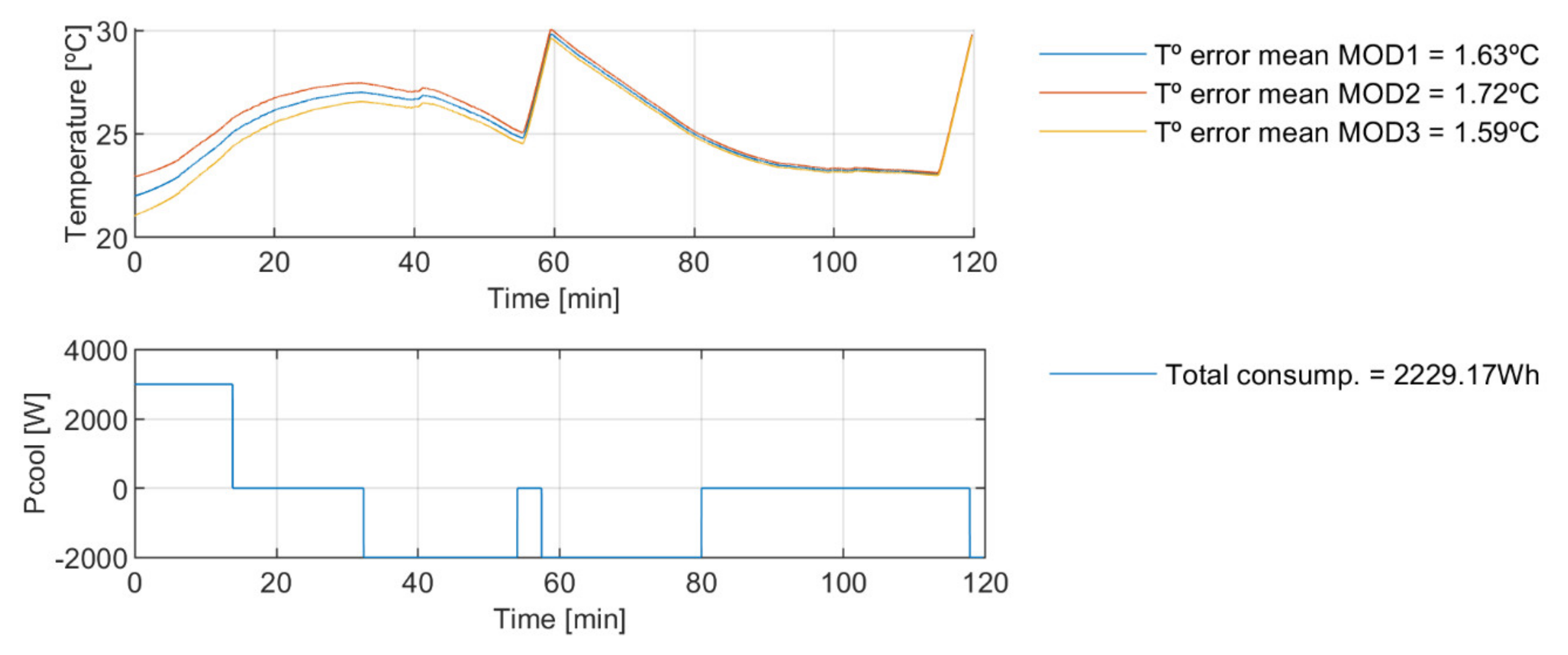
.) even though both traditional controllers could only manage one input. Both traditional controllers got feedback from the temperature measurement of the first module. The results of the proposed state diagram controller, with a ±2 °C threshold tolerance, are shown in Figure 8. The obtained average temperature error was 1.63 °C and the total thermal energy consumption was 2.23 kWh. The results of the tunned PID controller in Section 3 are shown in Figure 9. The obtained average temperature error was 1.06 °C and the total thermal energy consumption was 3.66 kWh.

Then, the proposal was tested. As the first step, the proposed control model was built. But before that, the data to build the model was generated. The model of the battery pack with the thermal management described in Section 2 was implemented in the data generation framework. The simulation restraints are listed in

Table 5. Simulation conditions.

Parameter	Values	Description
Troom	25 and 30	Room temperature.
Tcell_ini	18, 19, 20, 23, 24, 25, 28, 29, 30, 36, 37 and 38	The module temperature at the beginning of the simulation. The maximum temperature difference between modules was assumed to be 2 °C.
Tlq	10, 20, 26 and 30	The liquid temperature at the beginning of the simulation.
Tobj	25	The controller’s temperature objective.
Tlimit1	1	Acceptable minimum average temperature between modules used in LP.
Tlimit2	1	Acceptable maximum temperature variance between modules used in LP.

. A total of 89,792 labelled samples were generated.

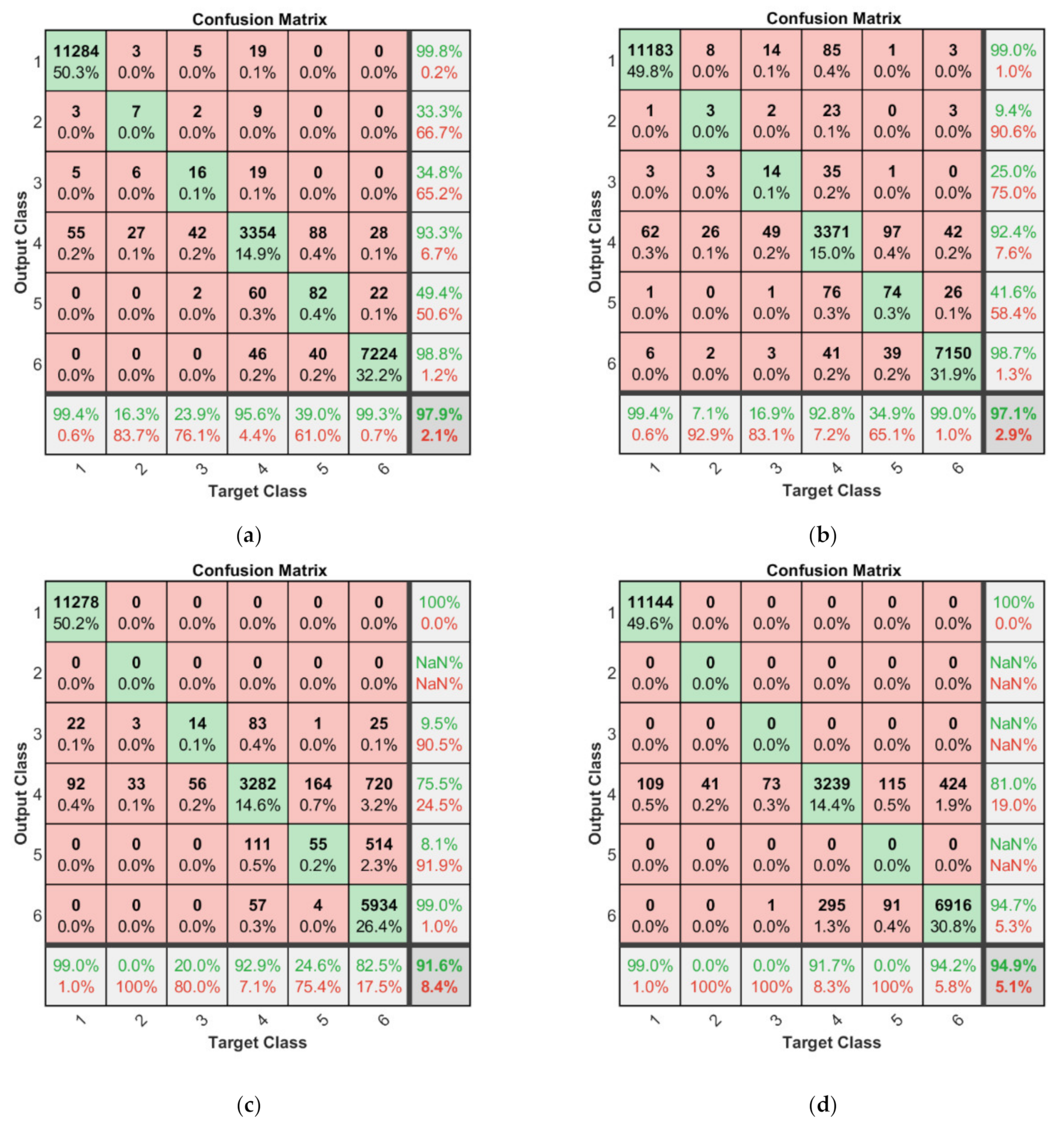
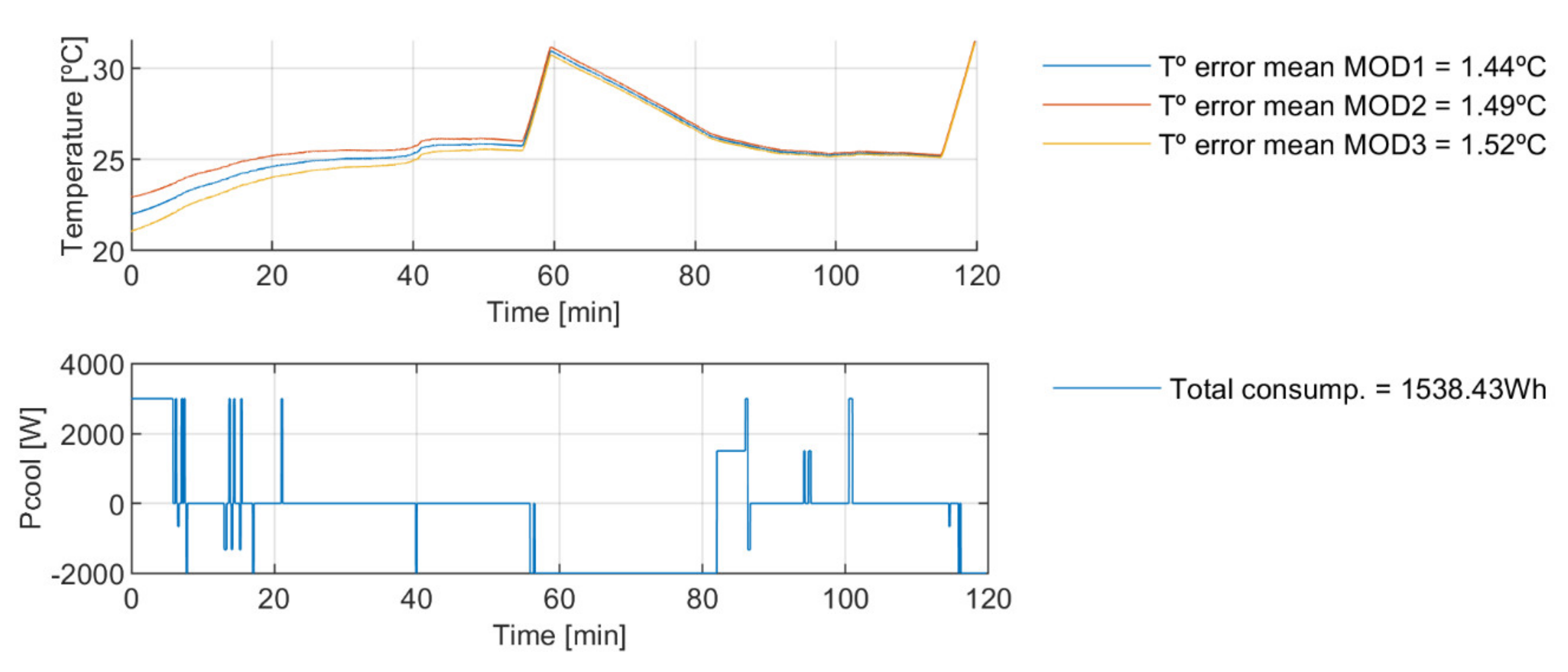
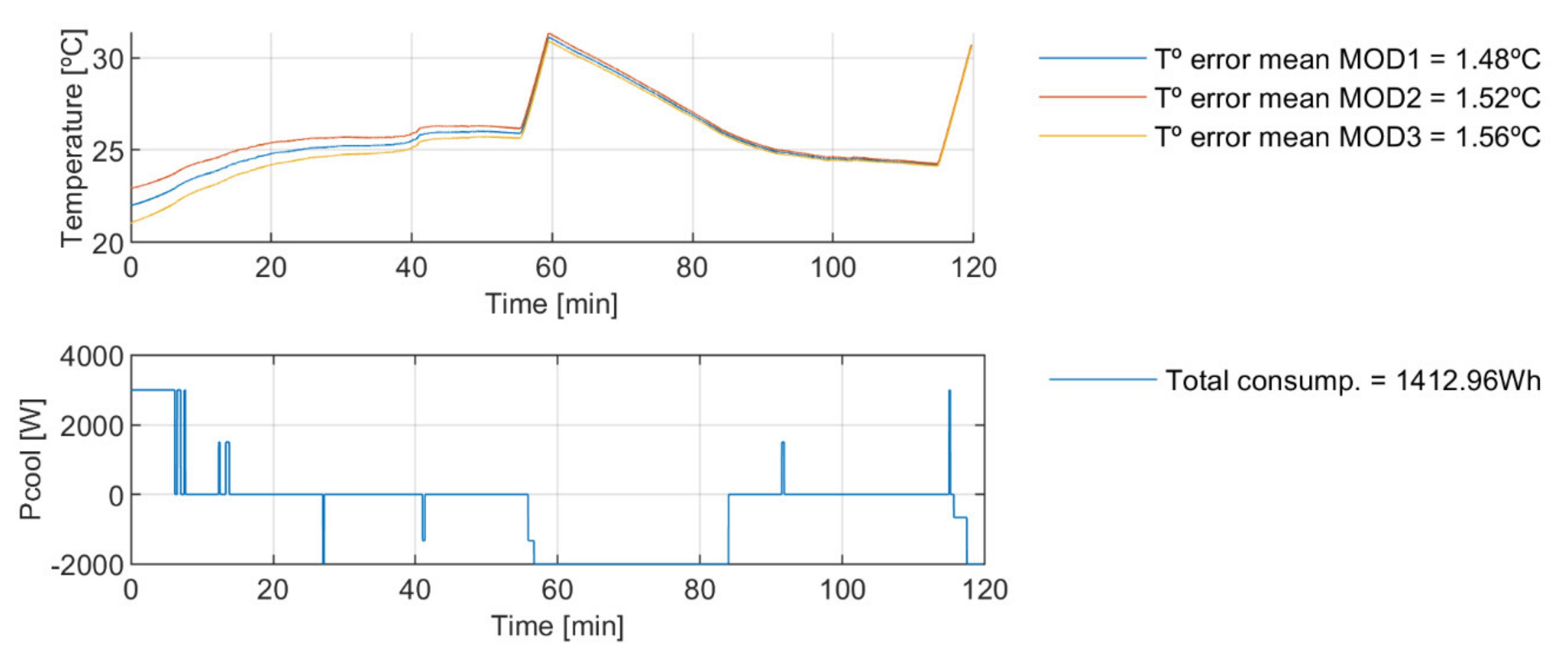
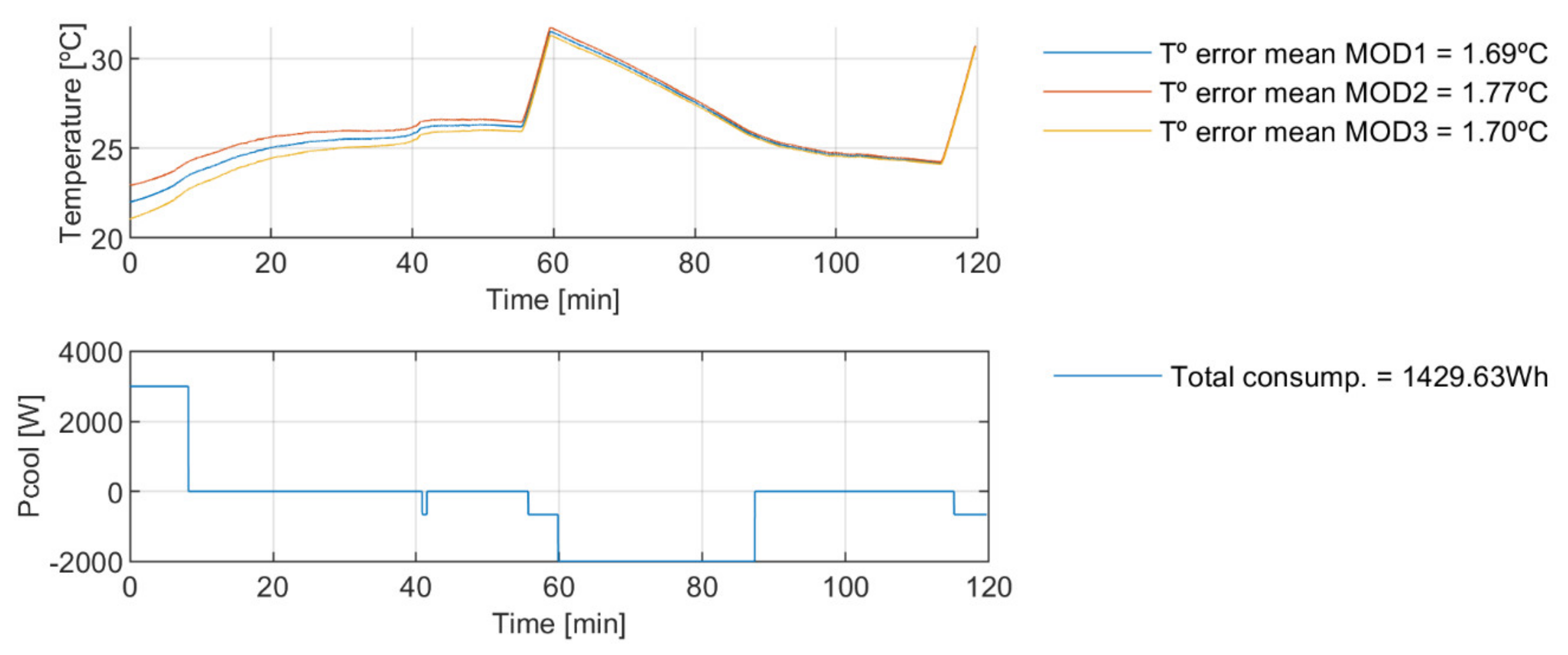
The generated data was used to build the proposed control model. For that, four different models were built using four different machine learning algorithms: a decision tree, a k-nearest neighbour, a naive bayes and a support vector machine. The models were constructed with MATHWORKS’ machine learning library named “statistics and machine learning toolbox”. The common practice of building these kinds of models is to split the data to have data for training and for validation purposes. Consequently, the data were split randomly into training data (¾ of the data, a total of 67,344 samples) and into validation data (¼ of the data, a total of 22,448 samples). The model was built using the training data. Then, the model was applied to the validation data. The results from the validation of the constructed models are quantified in a confusion matrix. These confusion matrices show the correct and incorrect guessing rates of the model, see Figure 10.

Afterwards, the proposed approach with the use case scenario was tested. For that, the constructed surrogate control models were applied in a simulation environment. The simulation operation conditions were the same as in the simulation of the traditional controllers (see Table 4). The obtained results are shown in Figure 11, Figure 12, Figure 13 and Figure 14.

6. Discussion

The evaluated traditional controllers showed good performance in keeping the battery temperature inside the safe operation window. The PID controller was maintaining the battery temperature at the set point (at 25 °C), except for when there was an ultra-fast charge. The total thermal consumption of the PID was 3.3 kWh. The state diagram, on the other hand, maintained the temperature inside the defined fuzzy zone instead of at the set point, except for when there was an ultra-fast charge. The total thermal consumption of the state diagram was 2.2 kWh. These behaviours were the expected ones. None of the applicable controllers can tackle the temperature rise in the ultra-fast charge due to the sizing of the chiller (out of the scope for the paper). Analysing them separately, it was seen that the PID was continuously activating the actuators to reduce the error of the controller, leading to high consumption values but low total deviations from the desired value. The state diagram controller, on the other hand, did not act in the fuzzy zone, leading to lower consumption rates than the PID, but higher total deviation from the desired value.

The construction of the proposed control model started with the data acquisition. The designed data labelling algorithm to generate the required labelled data consisted of testing all possibilities and selecting the optimum one. It shared many similarities with a MPC, but without restraints in the number of simulations. This meant that the proposed labelling algorithm exceeded greatly the computational burden of a MPC (which was already high), making it non-viable for on-board applications as an actual controller. Nonetheless, the results from this kind of simulation environment are global optimum responses for MIMO systems, which can be used to develop surrogate control algorithms that outperform the traditional ones in control capabilities.

The proposed control model was built with four different basic machine learning classification algorithms. Each of the models were built using ¾ of the generated labelled data. It should be highlighted that the division of the data was done randomly. This meant that the training data used to construct each of the machine learning based control model was different. In addition, the training itself can lead to different solutions even though using the same training data. Consequently, the result evaluation must be done qualitatively rather than quantitatively, even though we can compare quantitatively the results of the confusion matrices. The confusion matrices show that the model with the highest correct guessing rate was the model built with the decision tree classification algorithm, and the lowest the one built with the naive bayes classification algorithm. This meant that the most interesting model would be the one built with the decision tree algorithm. Nevertheless, the differences were relatively small (all of them had a correct guessing rate above 90%).

Analysing the confusion matrices more deeply, it was observed that there were three labels that the constructed models were able to guess correctly with rates of 90% or above and that there were another three labels that the model was not able to guess so well (correct guessing rates below 50%, having cases of 0%). At the same time, it was observed that the number of the labelled samples at those labels differed relevantly. The correct guessed labels had much more labelled data samples behind than the other ones. This means that most of the labelled data was focused on those three labels, leading to a model that got high correct guessing rates by only describing properly those three labels. Therefore, even though there were labels with considerably low correct guessing rates, the total correct guessing rate was high. Consequently, the models were expected to show average high-performance rates, but at the same time, the models were expected to show uncertain performance rates in the exceptional cases where the three labels that the model cannot properly describe were required.

The constructed control models based on the proposal were tested by simulating the use case scenario. The results showed that the developed controller maintained the temperature inside the safe temperature operation window (5 to 48 °C), where a MIMO system with invariances was controlled. It was observed that the invariances decrease all by themselves with time and they do not increase after the ultra-fast charge events. This was happening because the differences of the battery modules do not generate enough imbalances to overcome the passive balancing capability of the BTMS. Nonetheless, the results showed that the proposal was able to observe these invariances and act accordingly.

The comparison between the proposal and the evaluated traditional controllers showed the potential of the proposal. The proposal attained a higher average control error than the PID controller: 50% higher average control error. Nevertheless, the maximum temperature in both cases is the same (there is less than 0.5 °C of difference) while the proposal consumed considerably less than the PID controller: 60% less. The proposal achieved almost the same average control error as the state diagram controller. The maximum temperature in both cases was the same as well (there was less than 0.5 °C of difference). However, the proposal consumed less than the state diagram controller: 35% less.

7. Conclusions

Traditional controllers such as the evaluated ones (state diagram controller and PID controller) have features that make them suitable to control the BTMS and their simplicity makes them very attractive. They ensure that the battery is safely operated (as observed in the results), and both can be implemented easily on commercial BTMS. Nonetheless, these kinds of traditional controllers are far from optimal. State diagram controllers have little flexibility, and they require deep knowledge of the system. PID controllers only focus on one aspect of the control, and they neglect the other control factors. Both have limitations when balancing the thermal inhomogeneities and they are incapable of actively minimizing the total consumption.

The proposed surrogate control model tackles these deficiencies. It can control MIMO systems with optimum decision-making assessments, minimizing the consumption while maintaining the safe operation of the battery and imposing almost noncomputational cost to the microcontrollers. Consequently, all four control challenges of a BTMS controller are covered (MIMO system, safety, minimum energy consumption and low computational cost).

The proposal provides a novel approach in the use of machine learning techniques with the purpose of surrogating a BTMS controller. The proposal focuses on the thermal homogeneity, safety concerns and range anxiety. Nonetheless, the paper describes a versatile methodology to construct a surrogate decision-making process. Firstly, it can accept other optimization constraints. Secondly, it can be implemented in any kind of industrial application.

Additionally, the fact of being a supervised classification model built with machine learning algorithms means that the training datasets can be lengthened with data obtained from on-board applications, or from further off-board simulations. This allows a continuous improvement of the controller. The controller is able to evolve.

In future further work, several aspects of the proposed approach will be improved. Firstly, the number of data samples under the same label should be controlled. It is important to label all the possible states where the controller will need to make a decision (the extrapolations are well known to be a problem on these kinds of models). However, the results show that a second round of simulations restrained with the knowledge obtained from the first round would enrich the labelled dataset. The cherry-picked samples based on expert knowledge gained from the first round will allow the construction of a more proficient model. Secondly, some assumptions were made in terms of the model complexity. The increase of the model complexity increases linearly with the simulation time and exponentially with the number of simulations. Nowadays, this is a challenge, which will be solved in the near future thanks to the exponential increase of the computational speed of commercial workstations.