Article

Translating Global Integrated Assessment Model Output into Lifestyle Change Pathways at the Country and Household Level

by
Clare Hanmer
1,*,
Charlie Wilson
1,2,
Oreane Y. Edelenbosch
3 and
Detlef P. van Vuuren
3,4
1
Tyndall Centre for Climate Change Research, University of East Anglia (UEA), Norwich NR4 7TJ, UK
2
International Institute for Applied Systems Analysis (IIASA), A-2361 Luxemburg, Austria
3
Faculty of Geosciences, Copernicus Institute of Sustainable Development, Utrecht University, 3584 CS Utrecht, The Netherlands
4
PBL Netherlands Environmental Assessment Agency, 2594 AV The Hague, The Netherlands
*
Author to whom correspondence should be addressed.
Energies 2022, 15(5), 1650; https://doi.org/10.3390/en15051650
Submission received: 13 November 2021 / Revised: 10 January 2022 / Accepted: 9 February 2022 / Published: 23 February 2022
(This article belongs to the Special Issue Energy Planning)

Abstract

:
Countries’ emission reduction commitments under the Paris Agreement have significant implications for lifestyles. National planning to meet emission targets is based on modelling and analysis specific to individual countries, whereas global integrated assessment models provide scenario projections in a consistent framework but with less granular output. We contribute a novel methodology for translating global scenarios into lifestyle implications at the national and household levels, which is generalisable to any service or country and versatile to work with any model or scenario. Our 5Ds method post-processes Integrated Assessment Model projections of sectoral energy demand for the global region to derive energy-service-specific lifestyle change at the household level. We illustrate the methodology for two energy services (mobility, heating) in two countries (UK, Sweden), showing how effort to reach zero carbon targets varies between countries and households. Our method creates an analytical bridge between global model output and information that can be used at national and local levels, making clear the lifestyle implications of climate targets.

1. Introduction

The Paris Climate agreement has set out goals of limiting global warming to well below 2 °C and requires each country to maintain nationally determined contributions to greenhouse gas reductions over time [1]. Stringent climate targets require major demand-side transformations [2,3,4]. As energy demand is directly related to energy used in everyday life, these pathways imply significant changes in lifestyle [5,6]. The model-based scenarios used to explore the implications of the Paris climate targets provide aggregated projections of energy demand. There is a gap between these abstract parameters and information about change at the household level consistent with the long-term targets. The high-level scenario output for global regions does not indicate how energy demand varies in different geographies or across heterogenous household types.
In this paper, we introduce a multi-step 5Ds method to translate energy demand for global regions as output from global integrated assessment models (IAMs) into information about lifestyle change at the household level in specific countries. The 5Ds stand for disaggregation (of sectoral final energy to specific energy services), downscaling (from region to country), decomposition (of service-specific final energy into activity, structure, intensity components), differentiation (into household archetypes), and description of detailed household-level lifestyle change. This novel combination of established techniques reveals differences between countries and household types, which are not visible in aggregated model output. Presenting implications for households provides a bridge between global scenarios and research on low-carbon lifestyles at the national and local levels.
Our method takes as a starting point IAM scenarios that describe the changes in energy and land-use systems required to meet the Paris targets. These scenarios play a key role in IPCC assessment reports and inform both international negotiations and target setting and national policies [7,8]. The scenarios are developed using modelling frameworks that represent interactions between human and environmental systems as well as between supply and demand-sides of the energy system. Typical reporting on the demand-side is at the level of final energy use for broad sectors such as transportation (passenger and freight) or buildings (residential and commercial). In terms of spatial resolution, global IAMs typically report results for 10–30 world regions, often resolving large countries such as China, India, and Brazil but otherwise reporting at continental or subcontinental scales. Public databases such as the IAMC 1.5 °C Scenario Explorer [9] make data at this level of granularity accessible across multiple models. Appendix A provides an overview of IAM models.
The gap filled by this research is to translate this high-level data into information relevant to households in specific countries in order to make clear the lifestyle changes implied by the aggregated scenario data. This provides a simple alternative to complex national energy system models. A wide range of energy models are used to support national planning and policy development [10,11]. National models enable detailed consideration of local context and policy priorities but do not provide the representation of energy prices, technology development and global carbon budgets available from integrated global models [12].
The novelty of our study is:
  • To develop and test a methodology for translating global IAM output into lifestyle change implications for households;
  • To recognise variation between countries and between different households in the effort required to reach net-zero targets;
  • To reveal differences between mobility and heating-related lifestyle changes within 1.5 °C scenario pathways.

2. Literature Review

2.1. The Demand Reduction Challenge

The Sixth Assessment Report of the IPCC demonstrates the urgency of reducing greenhouse gas emissions [13,14]. In 2019, global GHG emissions were dominated by the use of coal (42%), followed by oil (34%) and natural gas (22%) [15]. Ambitious scenarios for emissions reduction show the importance of reducing energy demand as well as decarbonizing energy supply [5,16]. Buildings were responsible for 25% and transport for 27% of global CO2 emissions in that year [15]. Changes in the way people use energy in everyday life are required to reduce these emissions [2]. The literature describing the changes required at individual consumption level highlights the magnitude of the changes in behaviour required [17,18,19]. Our research provides a method to present transformations in energy demand at a household level, to support communication with the public about the changes necessary in their country [20,21].

2.2. Analysing Energy Demand

Our 5Ds approach provides a quantitative pathway of change over time in energy services per household, bringing together precedents from disparate sources within the literature: disaggregation (from energy-services and energy-systems analysis), downscaling (from spatially-explicit modelling), decomposition (from sectoral demand analysis), differentiation (from bottom-up energy demand modelling), and description (from lifestyle narratives). Multiple steps are required in order to analyse energy demand across different dimensions of energy use sector and spatial scale. Chen et al. in this issue [22] demonstrate the power of decomposition to analyse average per capita emissions for global regions on a sectoral basis. Our analysis combines decomposition with additional steps to focus in on emissions for specific services from a variety of household types in a particular country.
The energy service approach is an established entry point into energy systems analysis, since useful service provision is the ultimate purpose of the energy system [23,24,25]. Energy is used in everyday life to provide services to users such as mobility, heating, and cooling. Downscaling results from a larger to smaller geographic areas is common for many different types of spatially explicit analysis (see, for example, Hoskins et al. [26] on land use, and Byers et al. [27] on vulnerability to climate change).
Energy demand at the service level can be decomposed into activity (A), structure (S), and intensity (I) components that distinguish respectively the quantity, type, and efficiency of service provision. This approach draws on a long tradition of ASI decomposition in energy demand analysis and modelling, notably in transport where activity is quantified in passenger-km, structure is expressed as a mix of alternative modes, and intensity is related to fuel efficiency per mode [28,29]. ASI decompositions are used in sectoral demand analysis and energy efficiency market reports to understand the relative contributions of different factors to changes in energy demand [30,31,32,33,34].
There can be significant variation of energy service use across households. This heterogeneity is considered in granular sectoral energy models that resolve a variety of socio-demographic and physical characteristics. For example, building stock models based on a set of dwelling archetypes are commonly used for bottom-up analysis of residential energy demand. Physical characteristics such as building fabric properties are key drivers of heating energy consumption for each dwelling archetype [35,36,37]. Vehicle stock models are core components of energy demand projections for the transport sector. These models consider the effects of income change over time and may include heterogeneity in physical determinants of travel demand such as urban or rural location, and access to public transport [38].
Information about energy demand pathways for particular household types provides opportunities for communication with the public directly relevant to their way of life [39,40]. Narrative storylines with quantitative underpinnings are powerful tools for communication and public engagement [17,41]. Lifestyle change pathways can also be used in deliberative contexts to explore the perceived feasibility, appeal, and policy requirements for low carbon futures [20].

2.3. Extending Global IAM Analysis of Low-Carbon Lifestyles

Integrated Assessment Models combine knowledge from multiple scientific and economic disciplines to provide reproducible scenarios for future energy use and the impact of this on the climate [42]. This includes a detailed representation of energy supply (see for example [43,44]), however the focus in this analysis is the IAM scenario results for energy demand.
Our approach complements existing work to extend the scope of IAM scenarios. Many IAMs come from an energy supply optimisation or computable general equilibrium modelling tradition, so they have a relatively coarse representation of energy demand [45]. However, in recent years, more detail has been included in the representation of energy demand such that more models now include subsectoral detail (e.g., passenger mobility by mode) as well as activity levels describing the quantify of energy service provided (e.g., passenger-kms) [46,47]. ASI decompositions have also been applied to compare drivers of change in final energy across IAM pathways [47,48].
Various approaches have been used to downscale IAM scenario output for global regions to countries or smaller geographic areas. For example, van Vuuren et al. [49] describe the use of simple algorithms to downscale population, income and emissions to national territories and 0.5° grid squares. Sferra et al. [50] downscale regional emissions to the country level using a reduced complexity optimisation model that mimics the framework of the IAM.
A common critique of global IAMs is that there is a lack of heterogeneous consumer agents or actors explicitly represented in the models [51,52]. Some IAMs do include certain types of household heterogeneity important for analysing specific research questions such as access to energy services between urban and rural households [53] or for households at different income levels [54]. Rising concerns around inequality and just transitions [55,56,57] are drawing attention to the importance for global models to capture within-country variation in the opportunities and capacities of different household types.
Recent collaborative initiatives between global and national modelling teams such as the CD-Links project [58,59] and the COMMIT project [12,60] have encouraged consistency between national and global scenarios. The 5Ds approach complements these activities by offering a simple technique to derive national results consistent with global models, without the specialist modelling resource required to link detailed models at the global and country level.
We contribute to the growing body of research considering lifestyle aspects of global IAM scenarios. Van den Berg et al. [61] distinguish the two main approaches used in global IAMs to-date. The first describes lifestyle changes in qualitative terms in scenario narratives, and then ‘translates’ those narratives into exogenous inputs or modelling assumptions such as reduced levels of activity [16,62] or increased levels of service efficiency [5]. The second approach simulates lifestyle changes endogenously as a function of changing technology costs, availability, or preferences [63,64]. Both approaches consider lifestyle change ex ante as a focus of the scenario or modelling exercise. Our 5Ds approach provides a complementary ex post or post-processing step that can in principle be applied to the output of any IAM scenario modelling, whether or not lifestyle change is considered ex ante. The stepwise approach differentiates service-level changes across heterogenous households within a country and so provides a higher resolution perspective on lifestyle change.
In the next section, we outline the five steps of this 5Ds method before providing illustrative examples of its application to heating and mobility energy services derived from a 1.5 °C scenario by the IMAGE model (a widely-used global IAM [65]).

3. Generalisable Method for Translating IAM Regional Output into Household-Level Lifestyle Change

3.1. Overview and Principles

The 5Ds method has five calculation steps to process IAM scenario output and a final communication step (Figure 1). Energy service use is derived for a household based on IAM totals for the base year (in the recent past) and one or more target years (the future end date of interest). Figure 1 shows the five calculation steps (including decomposition at both region and country level) before a final communication step of describing lifestyle change pathways.
The endpoint of the calculations is an activity-structure-intensity (ASI) decomposition of energy demand. Activity is defined as the amount of energy service, intensity as the final energy consumed for each unit of activity, and structure as the different combinations of fuel and technology used to deliver the service (identifying the share of total activity for each). Table 1 shows the ASI dimensions for heating and mobility.
Equation (1) shows structure S defined in terms of activity A. Each form of service–delivered with technology j using fuel f—provides a proportion Sfj of the total amount of service, defined as the fraction of the total activity AT.
S f j = A f j A T
Equation (2) shows the full decomposition, relating final energy E to total activity AT, the fraction of activity Sfj for each combination of fuel f and technology j, and the intensity Ifj for each combination or form of the service.
E = A T f j S f j I f j
The algorithm employed at each of the five calculation steps is selected based on the characteristics of the energy service. In each case, the algorithm is linked to an underlying assumption about how the variable of interest for the smaller unit (subsector, country or group of households) relates to that for the larger unit of which it is part (sector, region or country). Five basic types of algorithm are employed. These are summarized in Table 2 and are described further in Appendix B. The first algorithms correspond to the three types of generic downscaling algorithms described in van Vuuren et al. (2007) for translating data at large spatial scales to smaller spatial scales (country or grid level). These downscaling algorithms can be applied to “any process in which coarse-scale data is disaggregated to a finer scale while ensuring consistency with the original data set” [49]. Two additional types of algorithm are applied in cases where the calculation goes beyond applying a scaling ratio to the larger unit.

3.2. Detailed Steps in 5Ds Method, with Illustration of Each Step for Mobility

In this section, we outline the series of steps to derive energy demand for a particular service at the household level in a specific country in the target year. The starting point is the final energy for the end use sector and region of interest reported in the IAMC data template [66]. This indicates the minimum information likely to be available from global IAM output.
We illustrate the application of the method to passenger mobility. The illustrative example uses data from a 1.5 °C scenario from the IMAGE IAM, referred to here by the abbreviated name ‘1.5C Total’. This is the ‘All’ deep mitigation pathway described by van Vuuren et al. [16], which incorporates both lifestyle change and rapid electrification based on renewable energy. We selected this pathway as one that shows more marked changes in certain energy-service demands, but, as we noted earlier, our methodology applies equally to scenarios in which lifestyle change is not explicitly considered. Output from the ‘1.5C Total’ scenario for the Western Europe region is used to derive energy service use in the UK and Sweden. In Appendixs B through E, we provide further details of the calculations and the external data sources used for each step.

3.2.1. Step 1 Disaggregate

The first step is to disaggregate IAM sectoral final energy for a region to the level of a specific energy service (Figure 1). Linear scaling (Algorithm 1) is applied if the share of sectoral final energy for the energy service can be assumed to remain constant. The share is calculated from base year calibration data and then applied to the target year IAM sector total. For services where future energy use for the service is not expected to track overall sectoral trends, scaling based on a higher resolution sector model (Algorithm 3) is applied.

Illustration for Mobility

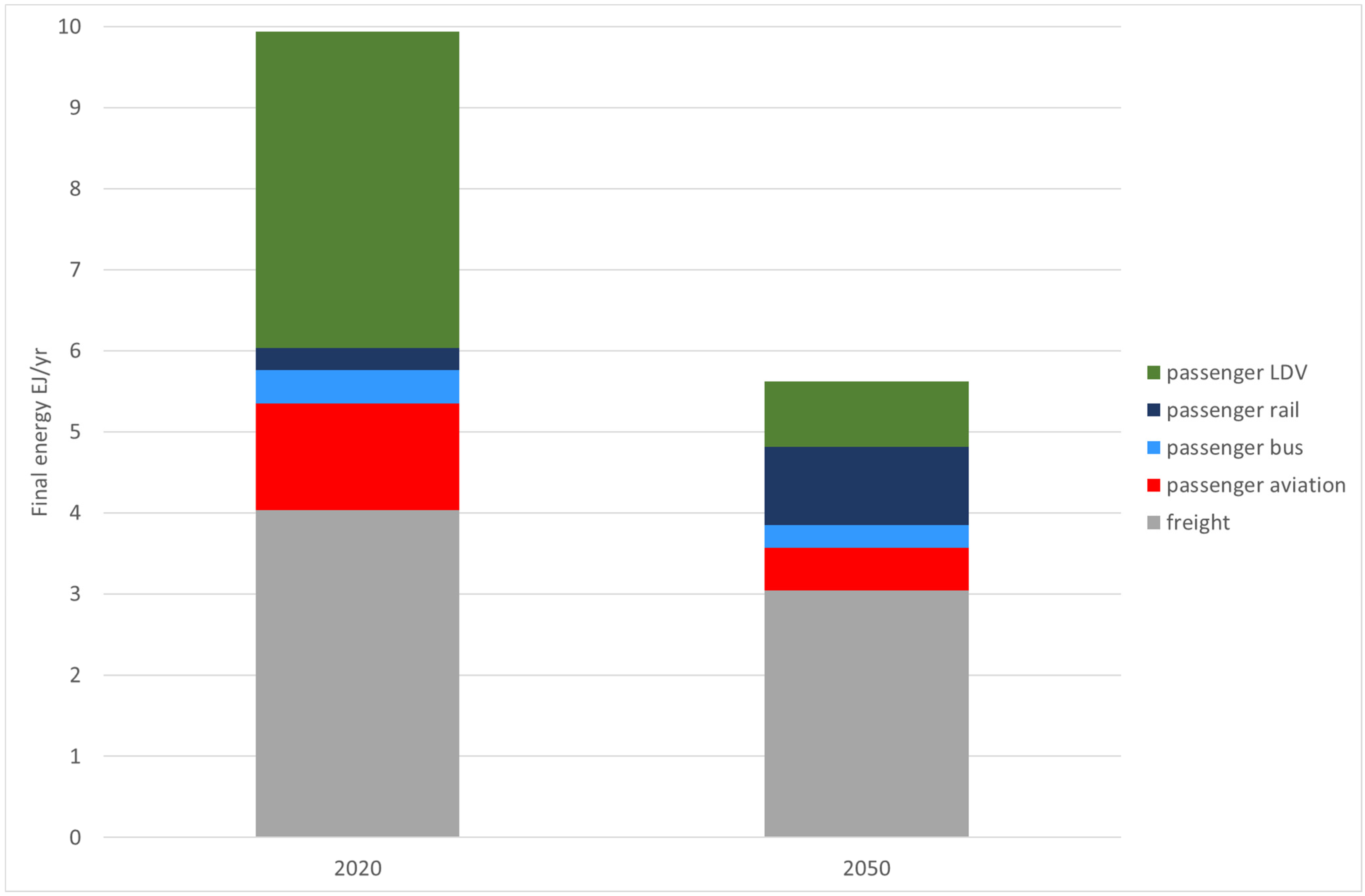
Figure 2 shows the results of the disaggregation step for the ‘1.5C Total’ scenario. Final energy for transport is disaggregated between freight and passenger mobility. There is no reason to expect the passenger mobility share of energy for transport to stay constant so a detailed scenario model for the target year is required to provide scaling ratios to apply to IAM final energy for transport (Algorithm 3). The assumptions and equations to derive final energy for passenger transport modes when these are not directly available from IAM output are outlined in Appendix C.

3.2.2. Step 2 Decompose for Region

Final energy for the region is decomposed across each combination of technology and fuel, establishing activity and intensity for each element of the structure (Figure 1). If both activity and final energy data are available from IAM output, intensity can be derived directly from this and no further calculations are required. Otherwise, intensity for each technology and fuel combination (for base year, and projected for target year) is estimated based on the literature. The energy balance for each fuel (Equation (2)) is then solved for activity (see Section 2.3 for heating, for which activity is known and the unknown is the building fabric property H). The term fuel as used in this report includes all energy carriers (such as electricity, hydrogen and heat) in addition to primary fuels (such as coal and natural gas). In cases where a fuel maps onto more than one form of service, a set of assumptions must be made about the allocation of the fuel across different technologies (e.g., electricity for mobility could supply electric LDVs, trains, or buses).

Illustration for Mobility

The generic decomposition Equation (2) expressed for passenger mobility is shown in Equation (3):
E = d T k f I k f   S k f
Activity is expressed in terms of distance d (passenger-km) travelled. E is the final energy for passenger transport and I is the intensity for mode k using fuel f (MJ/passenger km). Different modes k in this equation are equivalent to different technology types in the generic decomposition Equation (2). The structure Skf is the proportion of total distance dT travelled by mode k using fuel f.
To reduce the complexity of the example, transport fuel options are grouped into two categories: electricity and liquid (which combines all liquid and gaseous fuels including petroleum, biofuels, hydrogen, compressed natural gas). This distinction preserves the ability to analyse the transition to electric vehicles projected in 1.5 °C scenarios.
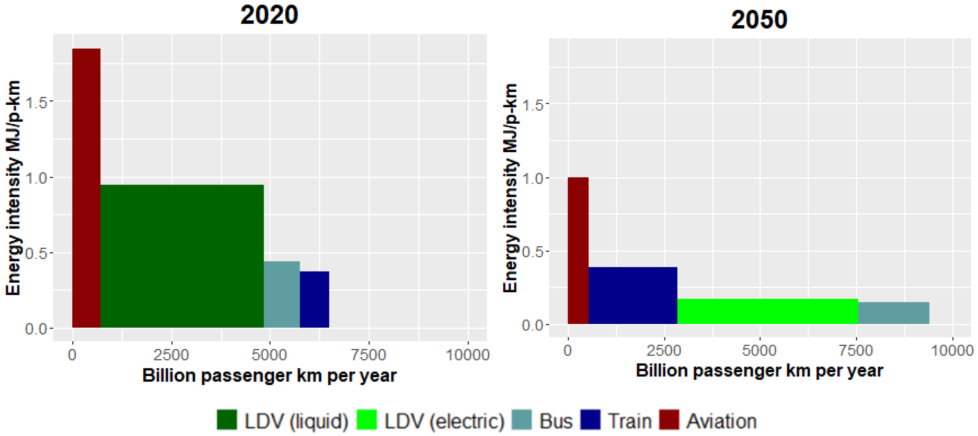
The IMAGE scenario output includes final energy and distance travelled (activity) for each passenger transport mode and fuel combination for the region in the target year, so transport intensity in the example is derived from this data, and there is no need for further decomposition calculations. Figure 3 shows the results of the decomposition step for the regional level.
Many IAMs report activity (distance travelled) and intensity (energy used per passenger km) figures for each mode of transport. In cases where the only output is aggregated across all modes of transport, so activity and intensity information for each mode are not directly available from the IAM, decomposition of mobility final energy for the target year involves solving a set of simultaneous equations. These are based on assumptions about the allocation of final energy for each fuel across different modes and matching the relative distances travelled by different modes with those from a detailed sector model. These assumptions and equations are detailed in Appendix C.

3.2.3. Step 3 Downscale

The next step is to downscale from region to country level (Figure 1). Household requirements for an energy service vary between countries in a region because of differences in factors such as climate, income, building stock characteristics, and typical travelling distances. The components of activity and intensity which vary by country are identified and the ‘scaling variable’ which represents these is established.
The downscaling step takes the total of the ‘scaling variable’ for the region and allocates this across countries in the region. The type of algorithm applied for downscaling is based on assumptions about whether the trends for energy use for the service in the country are likely to:
  • follow the same trends as the region as a whole (apply Algorithm 1);
  • converge on the regional mean (apply Algorithm 2);
  • diverge or otherwise follow irregular trajectories (apply Algorithm 3 by using external input from a higher resolution analysis of the specific energy service).
This follows the ‘simple algorithm’ approach laid out in Van Vuuren et al. [52].

Illustration for Mobility

For mobility, the quantity which differs between countries is the distance travelled by each transport mode and this is identified as the ‘scaling variable’. New vehicle technologies as well as efficiency standards are widely diffused, so it is assumed the intensity for each mode and fuel combination is constant across countries in a region.
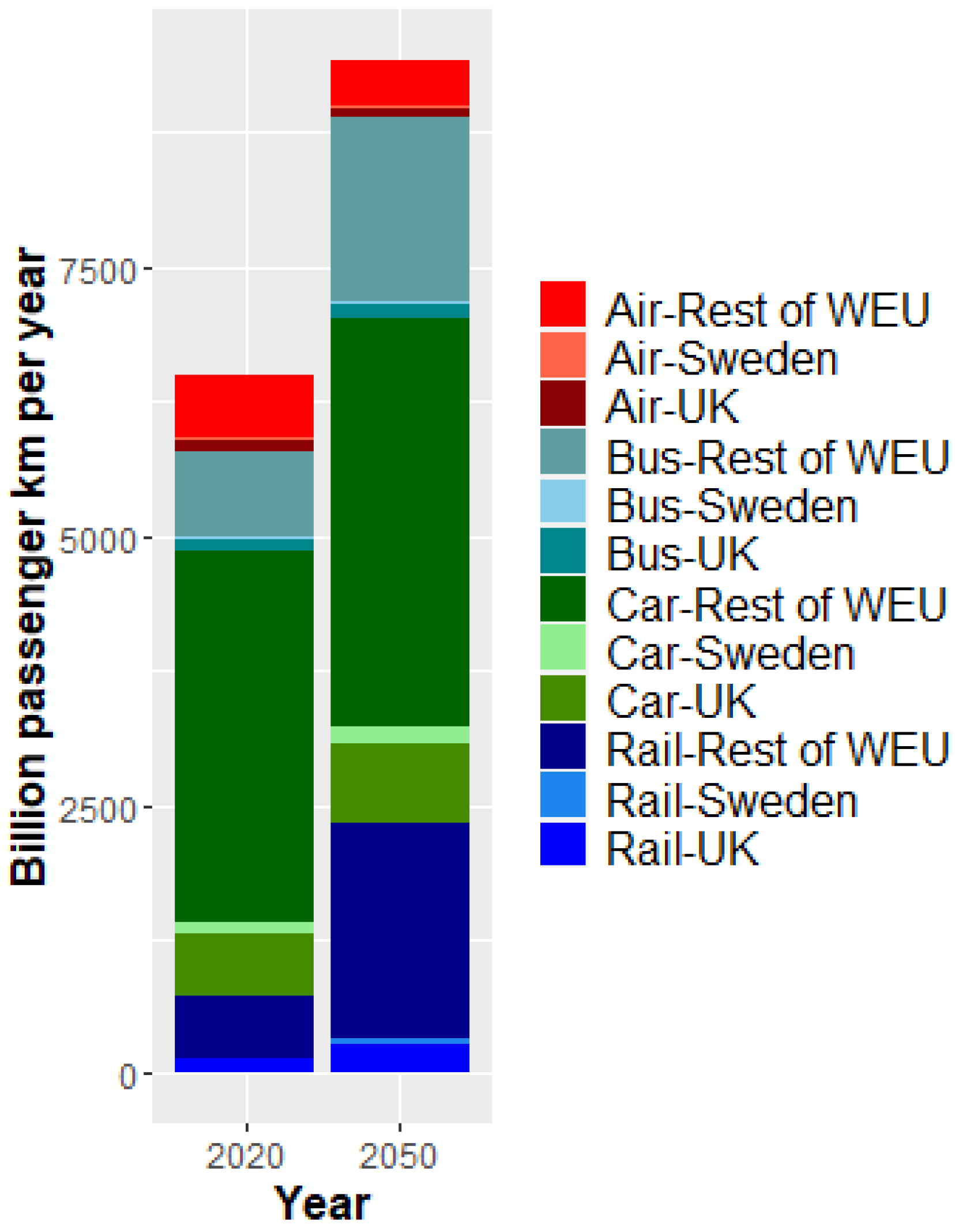
Future mobility patterns will be influenced by the evolution of current travel practices, vehicle stocks and infrastructure. This means it is unlikely that all countries within a region will follow the same trends or have the same mix of transport modes in the target year. The approach taken for downscaling the distance travelled from region to country is to use external input from a higher resolution scenario modelling analysis reporting country level results (Algorithm 3). This provides the country to region ratio of distance travelled by particular transport modes. This ratio is used to downscale the regional distance by mode (in passenger-km) derived from the global IAM scenario. The external input in this illustration of the method uses the Directed Vision scenario [67] This is a scenario describing strong policy action at the European level to deliver on the EU’s 2050 net-zero target; the scenario was interpreted by a suite of inter-linked sectoral and energy-system models, including ASTRA which resolves vehicle fleet and transport choices for 27 EU countries, which is broadly consistent with the IMAGE ‘1.5C Total’ mitigation outcome. Figure 4 shows the results of the downscaling step.

3.2.4. Step 4 Decompose for Country

Following downscaling, a second decomposition step at the country level is carried out (Figure 1). The unknowns and constraints for this decomposition are established based on the characteristics of the energy service considered. Local infrastructure constrains which forms of energy service are accessible. Energy infrastructure development is highly path dependent [68,69]. For services with infrastructure constraints, rules are applied to allocate future shares for each combination of technology and fuel (algorithm 5).
The country decomposition results can be used to assess the contribution of changes in activity, structure and intensity to the overall change in final energy. Ang [70] provides an overview of the development of ‘index decomposition analysis’ used by researchers to investigate trends in energy use. These techniques, developed for the analysis of historical energy data, have also been applied to emissions projections from IAM scenarios [47,48,71]. Appendix B.4 explains how the relative contribution of activity, structure and intensity effects can be calculated using the Sun method.

Illustration for Mobility

The mobility example illustrates how the country decomposition step draws on results from both the downscaling and regional decomposition steps. Mobility activity for the country is the sum of the distances by mode established in the downscaling step. As the 1.5 °C scenario used in this illustration sees rapid and pervasive electrification of the vehicle fleet, it is assumed that the electrified share of each mode converges to a regional average (established in the regional decomposition) by the target year of 2050. The structure is established by applying the regional electrified shares to the downscaled distances by mode for the country (e.g., splitting the distance travelled by LDV between electric and liquid fuel vehicles by applying the regional electrification ratio to the downscaled country distance travelled by LDV). As explained in the previous section it is assumed that regional intensities also apply at the country level. Infrastructure constraints are assumed not to apply.
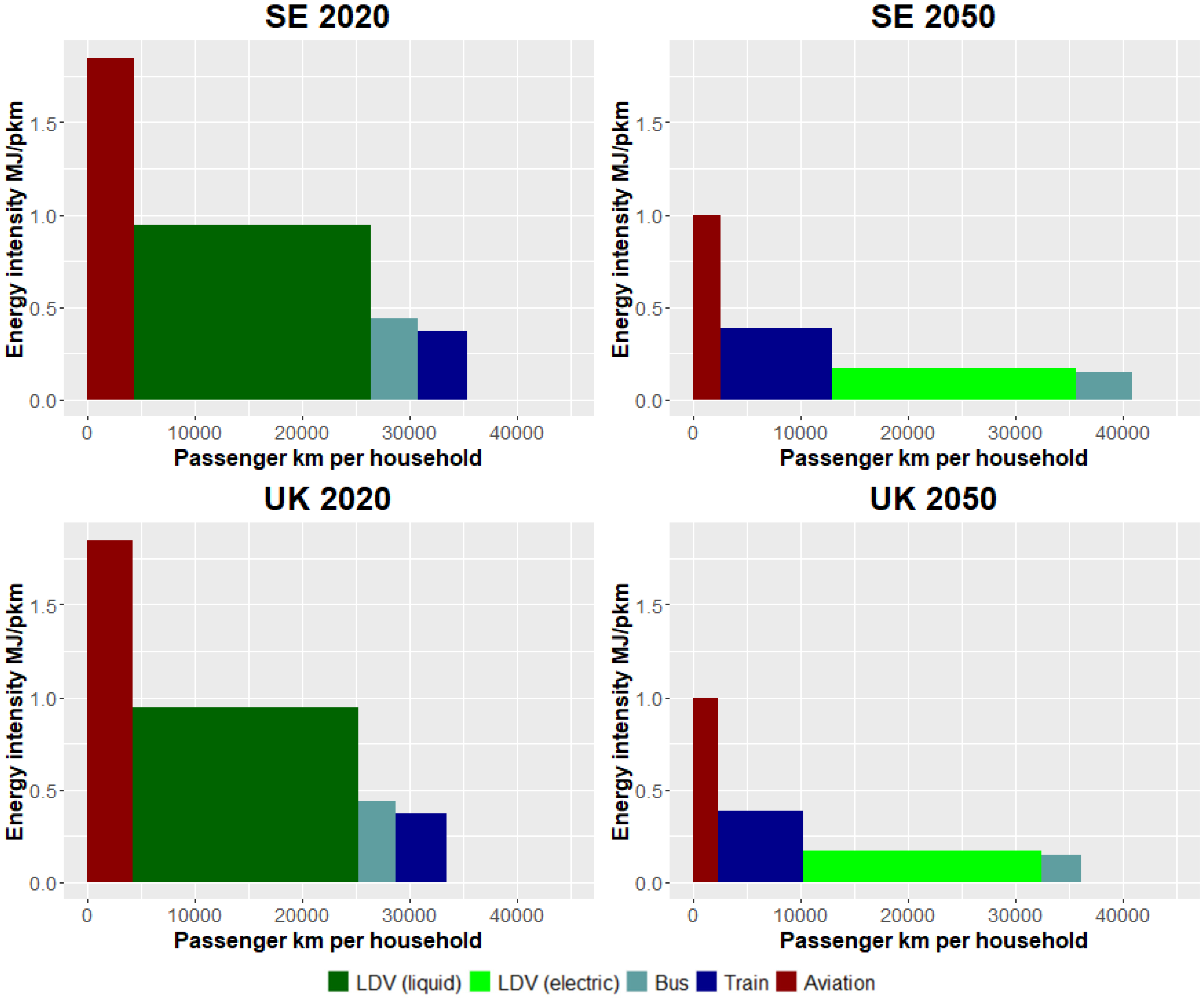
Figure 5 shows the results of the decomposition step, expressed as changes in activity, structure and intensity for mobility for two countries in the 1.5 °C scenario illustration. The household travel patterns in 2020 are similar in both countries. In both countries to 2050, overall activity increases but with very significant improvements in intensity projected at the regional level. There is a shift from LDVs using liquid fuels to battery electric vehicles, distance travelled by air reduces, and distance travelled by train increases. Table 3 shows the relative contributions of each ASI effect to the change in final energy. In both countries in this scenario the intensity effect (UK 45%, Sweden 48%) is significant, but lower than the structure effect (UK 62%, Sweden 66%). The changes in structure caused by the transition from petroleum fuels to electric vehicles provide the greatest overall contribution to reduction in final energy.

3.2.5. Step 5 Differentiate

The last calculation stage, differentiation, draws on sectoral modelling and empirical analysis to identify the main causes of variation in energy services across households within a country. Archetypes (groups of households) with distinct characteristics that shape the activity, structure, and intensity of their energy service consumption are identified. The dimensions of variation can be socioeconomic (e.g., income), geographic (e.g., urban), or physical (e.g., building type). These are combined to create a simple set of household archetypes (e.g., eight archetypes along 2 × 2 × 2 dimensions of variation). The share of national activity for each form of service for each household archetype in the base year is established by drawing on household surveys and other national data.
The target year final energy at the country level is differentiated across this set of household archetypes, with activity, structure and intensity established for each. The ‘scaling variable’ for the service (see step 3) indicates the components of activity and intensity that vary between archetypes. The algorithm to project the ‘scaling variable’ from base to target year is selected based on the characteristics of the service and decisions on whether differences between archetypes are likely to persist.
For some services, infrastructure or other physical constraints affect the suitability of different forms of service to a particular archetype (e.g., access to necessary infrastructure such as gas networks or electric vehicle charging points). In these cases, service-specific rules (Algorithm 5) are applied to establish the structure for the archetypes in the target year. In the mobility example, it is assumed there are no archetype-specific constraints; in other words, each archetype has equal access to electric vehicles and charging infrastructure. It is also assumed that the country electrification ratio for each mode can be applied for each archetype, thus establishing the structure for each.

Illustration for Mobility

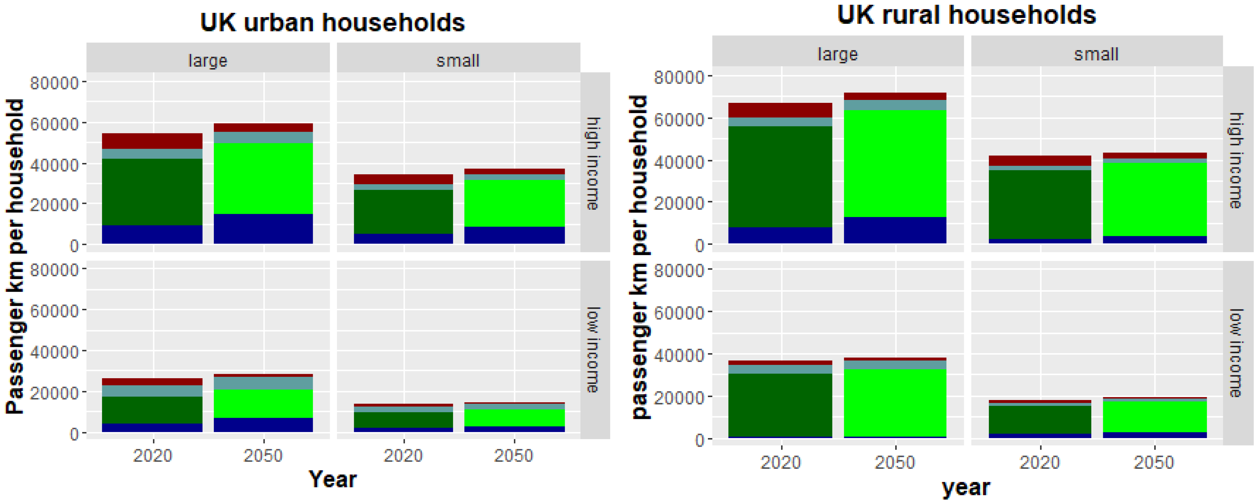
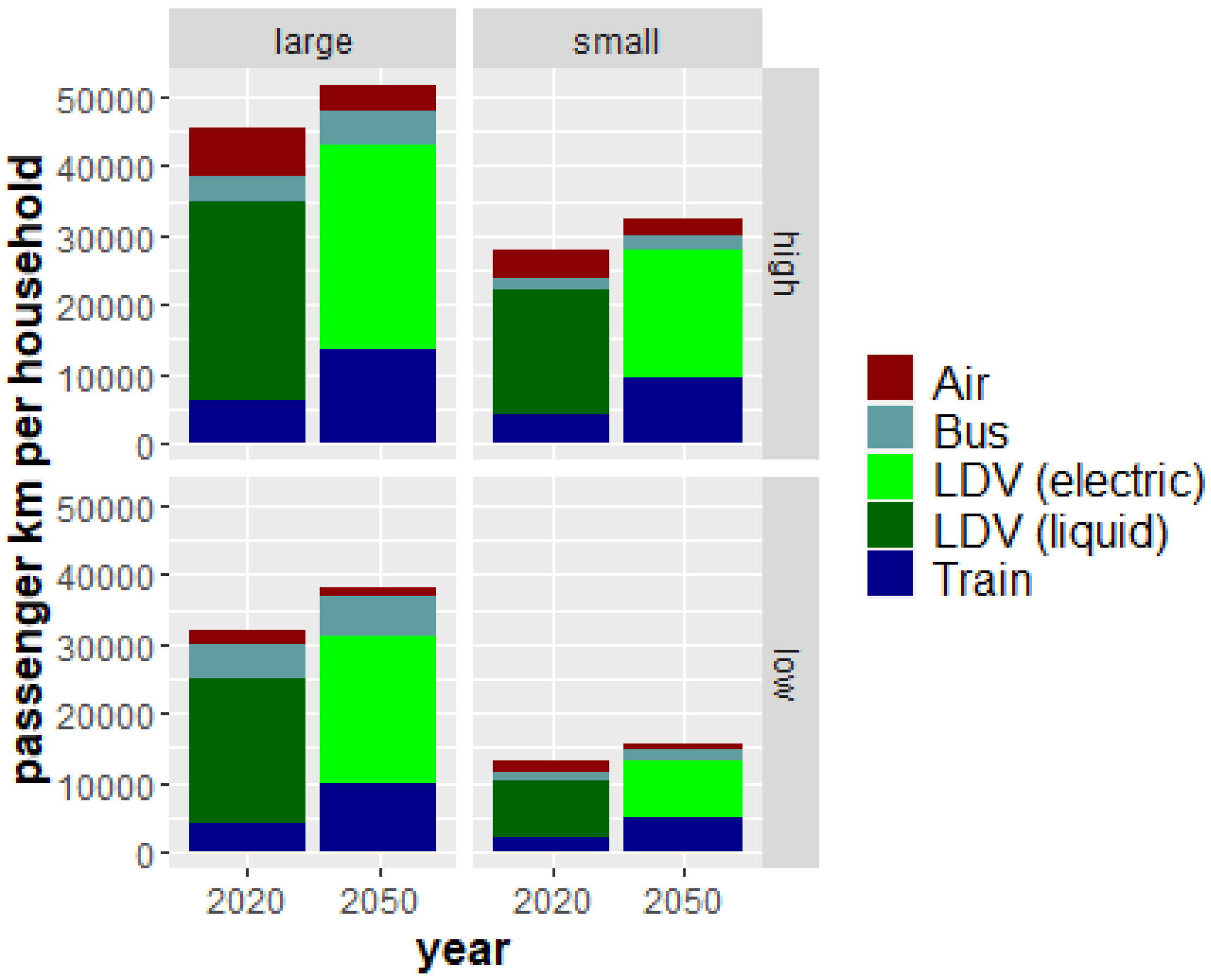
For mobility, archetypes are differentiated based on household size and income, urban or rural location, all factors which are known to influence distance travelled. The distance travelled by mode (the ‘scaling variable’) by each archetype in the base year is established from survey data characterising the heterogeneous travel behaviour of a representative set of households, such as the National Travel Survey in the UK [72]. In the illustration it is assumed that income and location differences persist so that each archetype’s share of the country total distance by mode is the same in the base and target years (algorithm 1). It is also assumed that average intensity for each mode and fuel combination is the same for each group of households. Figure 6 shows the different activity level and structure for eight UK household types in 2020 and 2050 from the 1.5 °C scenario illustration, with higher activity levels associated with larger households, higher incomes, and a rural location. Figure 7 shows distances travelled by four Swedish archetypes.

3.2.6. Step 6 Describe

In the final communication step, quantitative descriptions of changes in the activity, structure, intensity components of energy services between base and target year are developed for each household archetype (Figure 1). This enables audiences to compare the impact of the modelled scenario on different types of household and to identify the likely impact on lifestyle for households like their own. Narrative storylines derived from the IAM scenario provide context and interpretive detail.
The ASI decomposition results also enable messages about lifestyle changes to be positioned in terms of the Avoid-Shift-Improve framework, which has been widely used to characterize interventions and policies for changing energy demand [17,73]. Actions consistent with given warming outcomes can be described in three categories:
  • avoid activity by reducing how much service is used;
  • shift within structure by choosing a lower energy form of service provision;
  • improve intensity by using a more efficient technology.

Illustration for Mobility

The use of the Avoid-Shift-Improve framework can be illustrated for the UK mobility results shown in Figure 5 and Figure 6. In this case, rather than showing an ‘avoid’ story, the overall distance travelled (activity) per household increases by 8% between 2020 and 2050. The narrative of change is about major shifts between modes of transport, for both private and public modes of travel. In the case of private vehicles, the ‘1.5C Total’ scenario shows a complete replacement by 2050 of cars fuelled by petrol and diesel with battery electric vehicles. The lifestyle implications of this change can be described, for example, by pointing out that households will need to integrate vehicle charging in their regular routines, rather than filling up their cars at petrol stations. Charging points will become important elements of local infrastructure [74]. For public transport, there is a significant increase in distance travelled by train (67% for the UK example) combined with a halving of travel by air. In 2050, holidays and business travel involving flights are less frequent. In lifestyle terms, a shift in long distance travel from plane to train is likely accompanied by changes in attitudes, with local holidays and virtual meetings perceived as satisfactory alternatives to trips to other countries.
The steps for the 5Ds method as applied to mobility are summarised in Table 4.

3.3. Application of 5Ds Method to Heating

The same principles and series of steps illustrated for mobility can be applied to other energy services such as residential space heating, with differences in the characteristics of specific energy services leading to differences in implementation. In this second illustration, we show briefly how the 5Ds method is applied to residential space heating. Full details for each calculation step are provided in Appendix D.
For heating, the starting point for disaggregation is final energy for the commercial and residential sector (reported in the standard IAMC template). For downscaling, the space heating requirements in a country depend not only on the heated floor area but also the climate and the building fabric properties (a poorly insulated building stock requires more energy to heat than a well insulted one in the same climate).
The generic decomposition Equation (2) expressed for residential heating is:
E = a T   H j f S j f η j f
E is final energy for space heating and Sjf is the fraction of total floor area aT heated by technology j using fuel f. The amount of heating service received by building occupants from a fixed amount of energy depends on both the (active) efficiency of the heating conversion technology (η) and the (passive) efficiency of the building fabric [75].
For the differentiation step, the variation between archetypes of space available and access to infrastructure is considered. For example the economics of district heating mean that it is best suited for densely inhabited urban areas with large numbers of smaller homes, while costs to supply more widely spaced, larger homes would be higher. Analysis of space heating structure enables a description of how the proportion of each archetype which use a particular heating system changes over time and how this will affect the everyday life of the households involved.
Using the IMAGE ‘1.5C Total’ scenario to illustrate the results of these steps, Table 5 shows the relative activity, structure and intensity (ASI) effects expressed as a percentage of the overall change in final energy. Activity at the household level does not change as it is assumed that floor area per household does not change from 2010 to 2050 in these two countries.
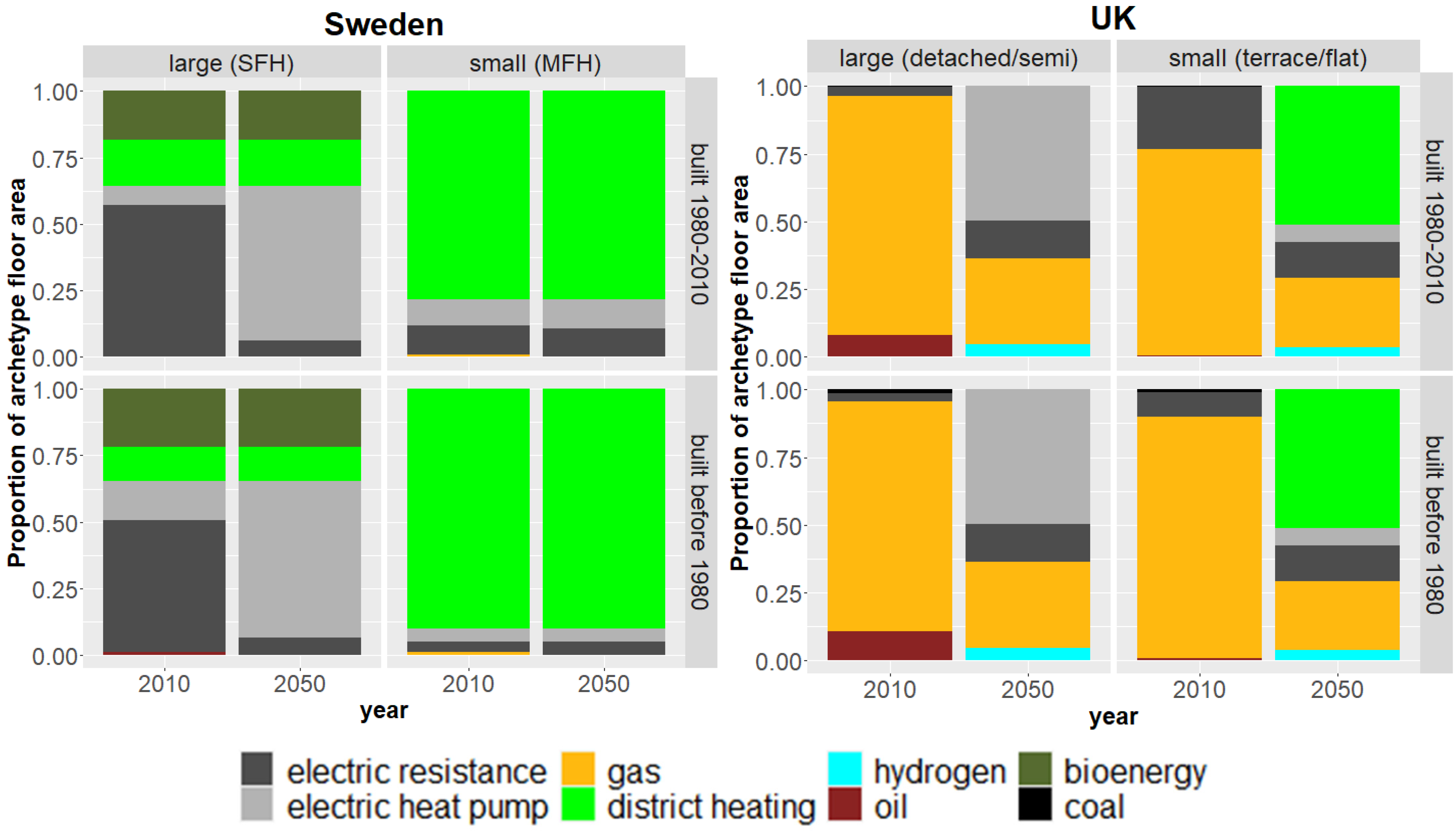
Figure 8 shows the change in heating types for the UK and Swedish housing archetypes. In Sweden low carbon heating options are currently in widespread use and district heating infrastructure is already in place. This is reflected in the very low percentage change projected for the structure component in Table 5. In the UK, much greater shifts in structure are apparent for all archetypes, in line with the national shift away from gas heating.
Table 5 shows that the energy reduction in Sweden is dominated by the intensity effect, and intensity change also contributes 72% of the UK reduction, highlighting the importance of improvements in building fabric to improve intensity. Activity at the household level does not change as it is assumed that floor area per household does not change to 2050 in these two countries. Based on the UK archetypes shown in Figure 8, the description for each type of house introduces the heating systems projected for 2050, with resulting implications for lifestyle change. For example, in the majority of larger homes where a gas boiler is replaced with an electric heat pump, households are likely to notice changes in the patterns of heating in the home associated with lower radiator temperatures and requirements for demand management of electrical heating [76,77,78].

3.4. Uncertainties in Results

Since the principle of the method is to divide up the total emissions from the IAM scenario across households the uncertainties associated with the global scenario projections also apply to the 5Ds results. Wilson et al. [79] provide an overview of methods for the evaluation of IAM models. Sensitivity to scenario assumptions and uncertainties in calibration data for the IMAGE model have been the subject of detailed analysis [75,76].

4. Discussion

This section discusses the general applicability of the method and its relevance for national policy making and for lifestyle research. We reflect on the results of the illustrative example and the opportunities for communication with the public.

4.1. General Applicability

We have illustrated the 5Ds method here for two countries (UK, Sweden) within a single global region (Western Europe). However, the method can be generalised to any country in any global region, and is also flexible to work with any global modelling analysis reporting sectoral final energy at the regional level. The principles of the 5Ds method can also be applied to energy services beyond mobility and heating (see Appendix F for further discussion). Sectoral modelling of energy use in buildings often distinguishes hot water, cooling, cooking, lighting, and appliances as well as space heating [80,81,82]. The 5Ds method enables more detailed consideration of the energy services associated with these categories than is visible in standard IAM output. It allows lifestyle changes for countries and households implied by different scenarios and models to be compared in a standardised way, for example exploring the trade-offs between scenarios emphasising supply-side transformation (e.g., [83]) versus demand-side transformation (e.g., [5]).

4.2. Benefits for National Policy Analysis

The 5Ds method provides country-specific information within a consistent global context since it derives national energy service data from global IAM output. This is relevant for national policymakers and researchers interested in the local impact of global scenarios. The long-term viewpoint from global IAMs (which typically provide projections up to 2100) can also provide an alternative perspective to national modelling, which is typically concerned with shorter timescales.
The ASI analysis can support national policy development and planning. Policy to reduce or avoid activity focuses on behaviour change, with a combination of information, incentives and “nudges” to make the desired behaviour easier [84]. A range of policy options are open to encourage a shift the structure to lower carbon forms of energy service. Economic incentives can influence consumer choice (for example when selecting a replacement heating system) while regulation–for instance, banning the sale of fossil fuel heating boilers after a particular date–can remove high emissions options [85]. Infrastructure planning is a crucial element in enabling shifts to low emission energy services. Many shifts cannot be achieved without the development of new energy supply infrastructure (e.g., electric vehicle charging points, district heating networks). An important policy lever to improve the efficiency of service provision is regulation in the form of product standards, as well as financial incentives and R&D funding, to improve the energy performance of technologies and service-provisioning systems [86].
The results for activity, structure, and intensity contributions to overall reduction in final energy in Table 3 and Table 5 illustrate how these may vary between countries, leading to different policy priorities. As an example, for heating the level of necessary infrastructure change in the UK is much greater than that in Sweden. There is less contrast between the countries in the components of energy reduction for mobility. In the ‘1.5C Total’ global scenario, both countries share a key priority of encouraging a shift to electric LDVs.

4.3. Lifestyle Change

As a post-processing step, the 5Ds method requires no changes to IAM code or modelling approach in order to communicate lifestyle change implications of mitigation pathways in more detail than is possible from standard IAM output. The information about changes in energy services at the household level is relevant for civil society actors interested in lifestyle change to achieve emissions reductions. The results are accessible for those who are not involved in policy and scenario modelling discussions. For example, the stringent mitigation scenario in the illustrations above shows households in the UK and Sweden travelling further by train but flying less than they do today.
The 5Ds method enables qualitative storylines of change at global, national, and local scales to be linked. The IAM scenario narrative provides an over-arching storyline about what is happening elsewhere in the world, within which the description of changes at the household level in a particular country can be situated. Global scenarios draw on reference pathways, such as the widely used Shared Socioeconomic Pathways (SSPs) [87]. The narrative for each pathway describes trends in the world economy, demographics and technology development. This provides a global context for energy services at national and household levels. For example, the ‘1.5C Total’ scenario (the starting point for the illustrations above) includes assumptions about rapid electrification in all end-use sectors and consumer changes in habits towards a lower greenhouse gas lifestyle [16]. These draw on an underlying narrative of co-operation between nations leading to rapid technology diffusion, and a shift in emphasis towards human well-being with less focus on economic growth. The 5Ds method adds stories about the changes in daily life that will be experienced by particular household types under the scenario.
The narrative can thus highlight both global and local conditions associated with the scenario. For example, the significant improvements in intensity for mobility seen in the ‘1.5C Total’ scenario result from technology development encouraged by government policy and international cooperation. Intensity intersects with lifestyle at the level of individual decisions about purchasing vehicles with high energy efficiency (or choosing these among shared mobility options). Low-intensity options will be encouraged by high carbon prices in this stringent mitigation scenario, and the scenario narrative also shows these decisions influenced by society-wide preferences for options with low environmental impact. The significant changes in intensity of heating energy in both the UK and Sweden imply major overhauls of the building stock in both countries, but households in the UK will have to adapt to new forms of heating, while Swedish heating types will change much less because low-carbon heating technology is already prevalent.

4.4. Limitations of the Method

Each of the calculation steps in the 5Ds method requires a series of assumptions on data inputs and data processing algorithms, which are documented in this article. These assumptions require a degree of background information and an awareness of the statistical information on the energy service being analysed to understand the infrastructural, policy, and behavioural context of future lifestyle change, as well as to calibrate base year assumptions.

5. Conclusions

5.1. Practical Implications of the Research

By translating results from long term global scenarios into national level projections for energy demand, the method offers a technique for national planning, highlighting the national infrastructure changes and policy priorities implied by the global model results and enhancing interpretability and usefulness of IAM results. The approach reveals differences between countries and household types which are not visible in aggregated model output, showing variation between mobility- and heating-related lifestyle changes within net-zero pathways.
The method broadens the potential audience for IAM scenarios to members of the public interested in changes in lifestyle. The energy service results enable a focus on how aspects of daily life such as residential heating or passenger transport will change over time. The identification of changes in everyday lifestyles makes IAM results more transparent for citizens, offering new ways to communicate scenarios to the public in a way that resonates with people’s lived experience. Details of the practical consequences for specific households are set within an overarching narrative about global emissions reductions and worldwide developments in population, economy, and technology.

5.2. Future Research Directions

The 5Ds method complements efforts to make global scenario modelling results publicly available. It can be applied to output from any IAM model, which reports energy demand, and to all types of mitigation and baseline scenarios. The purpose of the study was to develop, test, and demonstrate the methodology. The next steps for research are to apply the methodology to comparatively assess results across different scenarios and models as well as to extend the application to additional energy services such as illumination, cooking and cooling. The method could contribute to a multi-model comparison of IAM results, providing the basis to compare national and household level energy demand results (based on the same assumptions and calibration data) across an ensemble of different models. This would also allow systematic investigation of scenario uncertainty at the service level.

Author Contributions

Conceptualization, C.H. and C.W.; methodology, C.H., C.W., O.Y.E. and D.P.v.V.; software, C.H.; formal analysis, C.H.; data curation, O.Y.E. and C.H.; writing—original draft preparation, C.H. and C.W.; writing—review and editing, O.Y.E. and D.P.v.V.; visualization, C.H. and C.W. All authors have read and agreed to the published version of the manuscript.

Funding

This research was funded by the CAST Centre for Climate Change and Social Transformations (UK ESRC Grant ES/S012257/1), with additional funding from the Energy Demand changes Induced by Technological and Social innovations (EDITS) initiative coordinated by RITE, the Research Institute of Innovative Technology for the Earth (Japan), and IIASA, the International Institute for Applied Systems Analysis (Austria) and funded by the Ministry of Economy, Trade, and Industry (METI) in Japan. D.P.v.V. and O.Y.E. thank the KR foundation for funding the IMAGE-Lifystyle project, contributing to the paper. The APC was funded by IRENA.

Institutional Review Board Statement

Not applicable.

Informed Consent Statement

Not applicable.

Data Availability Statement

Data sources are listed in Appendix E.

Acknowledgments

Thanks to Vassilis Daioglou and David Gernaat, Netherlands Environmental Assessment Agency, for assistance supplying and interpreting IMAGE output data, and to Stephanie Heitel, Fraunhofer ISI, for her assistance.

Conflicts of Interest

The authors declare no conflict of interest.

Appendix A. An Overview of Integrated Assessment Models
Global integrated assessment models (IAMs) are tools for simulating the energy and land-use transformations that are necessary to limit global warming to meet climate targets. They represent linkages between energy, land use, climate, and [45,88]. IAMs are used to analyse long-term global climate outcomes under what-if assumptions about future drivers of change [79]. The Intergovernmental Panel on Climate Change (IPCC) fifth assessment report drew on 1134 scenarios from 30 global IAMs [42,89]. The 2018 IPCC Special Report on global warming of 1.5 °C drew on 411 scenarios from 10 global IAMs [90]. IAMs contribute directly to climate policy formulation, including UNFCCC international negotiations and national strategies and targets [91]. The models have been extensively peer reviewed and are increasingly open source.
IAMs typically have a high degree of resolution of energy supply. For example, the IMAGE IAM models 6 options for heating fuels, 17 different options for electricity generation, and 10 different forms of hydrogen production [92]. Efficiency and cost changes over time are modelled for energy demand. Transport demand is either based on top-down modelling (related to population and economic growth), or a hybrid with different technology options represented [47] (nine different passenger transport modes are represented in IMAGE [92]). Industrial demand sectors are represented in varying levels of detail (in the IMAGE model steel, cement and plastics production are each separately represented). Residential energy is the other major demand sector that is represented. Household income is a key driver for residential energy demand [54].
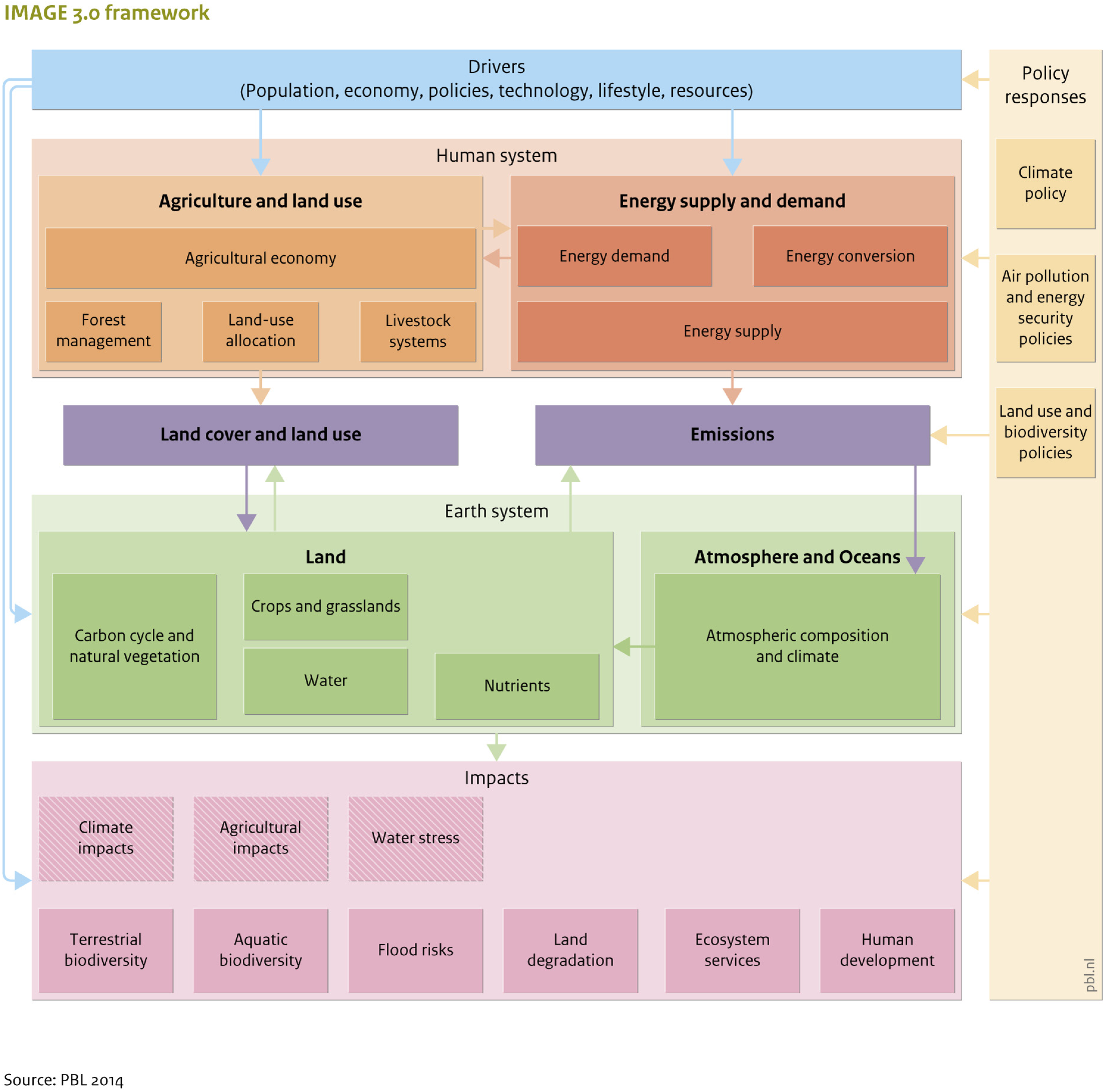
Figure A1 shows a schematic representation of the IMAGE IAM model illustrating how drivers are linked to impacts through human and earth systems. IAMs project a cost-optimized mix of energy supply given the scenario assumptions and climate target. A baseline scenario with assumptions for economic and population growth is chosen (frequently one of the Shared Socioeconomic Pathways [87]). Deep mitigation scenarios are implemented by introducing a uniform global carbon tax to meet the radiative forcing target associated with the specific climate target [16].
Figure A1. An overview of the IMAGE framework and its components, reproduced from https://models.pbl.nl/image/index.php/IMAGE_framework_summary (accessed 10 January 2021).
Energies 15 01650 g0a1

Appendix B. Principles of 5Ds Calculations

Table A1. Nomenclature for Appendices.
afloor area
Aactivity
Bfinal energy for bus
Cfinal energy for LDV
Efinal energy
Ffinal energy for freight transport
Hbuilding heating required per unit area
IIntensity
Ltotal final energy from ‘liquid’ fuels (incorporates gaseous fuels)
Ptotal final energy from electricity
Quseful space heat energy
Rfinal energy for passenger rail
Ttotal final energy for residential and commercial
SStructure
Vfinal energy for (passenger) aviation
εelectrification ratio–ratio of distance travelled by mode using electricity to total distance travelled by mode
ζratio of total energy for transport from IAM to total from detailed model
ηefficiency of heating technology / vehicle
subscripts
Ccountry
eelectric
ffuel
gfuel (excluding electricity)
Iderived from IAM
kconvergence year
lliquid
Mderived from detailed scenario model
pelectric heat pump
relectric resistive
Rregion
Ttotal
αarchetype

Appendix B.1. Technology and Fuel Combinations

The structure to which mobility energy use is decomposed is a set of mode and fuel combinations. The share of activity for the region, country, or household for each combination is derived for each combination (form of service).
The modes considered for passenger mobility are:
  • LDV (light duty vehicles, predominantly cars)
  • Bus
  • Rail
  • Aviation
The fuel options are grouped into two categories: electricity and liquid. The liquid category combines all liquid and gaseous fuels (petroleum, biofuels, hydrogen, CNG), and a uniform efficiency is assumed for all vehicles in the same mode using liquid fuels.
The structure dimension for heating is the share of the activity that is attributed to each combination of heating technology and fuel. Eight combinations are considered in this analysis:
  • Electric resistance heater
  • Electric heat pump
  • Gas boiler
  • Heat from district heating network
  • Hydrogen boiler
  • Oil boiler
  • Biomass boiler
  • Coal boiler

Appendix B.2. Base Year Selection

The heating illustration takes 2010 as the base year. Calibration was found for dates between 2010 and 2013 (see Appendix D), so 2010 is the closest date with IAM data available (IMAGE IAM scenario output is reported at decade intervals).
For mobility, a base year of 2020 was chosen. Detailed model scenario data was used for this year, rather than calibration data from national and international statistics. This overcame difficulties in finding consistent calibration data across all transport modes.

Appendix B.3. Calculation Algorithms

Algorithm type 1, linear scaling, assumes that the smaller unit represents a constant proportion of the larger unit. Algorithm type 2, convergence, assumes values for the smaller unit converge to an average value for the larger unit. Algorithm type 3 is based on external input from an alternative model or scenario with greater resolution of energy service demands and does not assume a simple linear relationship between smaller and larger units. The scenario narrative from this external model, particularly the level of mitigation stringency, should be matched as closely as possible to that of the IAM. Algorithm type 4 refers to the decomposition of energy service demand into activity, structure and intensity (Equation (2)). Algorithm type 5, rule-based allocation, is applied when the options for the smaller unit are limited by physical constraints such as the availability of fuel supply infrastructure. In such cases, a decision tree set of questions is followed to allocate appropriate fuels to the smaller unit.

Appendix B.4. ASI Contributions to Change in Final Energy

The analysis of ASI contributions follows the Sun index decomposition method [85] to divide up the change in final energy ∆E between base year b and target year t.
Δ E = E t E b
E is expressed as the sum of the effects due to activity, intensity and structure:
Δ E = E A e f f e c t + E I e f f e c t + E S e f f e c t
Each of these effects is expressed in terms of changes in overall activity A, intensity Ifj and structure Sfj summed across all combinations of fuel f and technology j.
E A e f f e c t = Δ A f j I f j b S f j b + 1 2 Δ A f j ( I b Δ S f j + S f j b Δ I f j ) + 1 3 Δ A f j Δ I f j Δ S f j
E I e f f e c t = A b f j S f j b Δ I f j + 1 2 f j Δ I f j ( S b Δ A + A b Δ S f j ) + 1 3 Δ A f j Δ I f j Δ S f j
E S e f f e c t = A b f j I f j b Δ S f j + 1 2 f j Δ S f j ( I b Δ A + A b Δ I f j ) + 1 3 Δ A f j Δ I f j Δ S f j

Appendix C. Additional Details of 5Ds Method Applied to Mobility

The main text provides an illustration of the 5Ds method applied to mobility using the ’1.5C Total’ scenario generated by the IMAGE IAM as an example. IMAGE reports mobility-specific data with more granularity than other IAMs. This appendix sets out the additional calculations needed if only aggregated sectoral IAM output is available.

Appendix C.1. Disaggregation

The starting point is regional energy used by mode from the detailed scenario output. This is used to disaggregate the IAM total energy for transport between four subsectors: freight, aviation, rail, and all road passenger transport (bus and LDV combined). It is assumed that the proportion of energy used by each sector is the same as that for the detailed scenario, and subsector totals are found by scaling detailed model amounts by ratio, ζ, of total energy from IAM to total energy from detailed model:
V R I = ζ V R M
C R I + B R I = ζ ( C R M + B R M ) etc .

Appendix C.2. Decomposition

If data for final energy for each transport mode is not available, a number of simplifications are made to derive a set of equations to relate total transportation liquid fuel final energy L and electrical final energy P for the region from the IAM scenario and the energy for each fuel for each mode.
Balance of liquid across modes:
LR = FlR + ClR + BlR + VlR
Balance of electricity across modes (assumes all trains are electric in target year, and there is no electric freight or aviation):
PRI = CeR + BeR + ReR
Two further assumptions are made:
  • The ratio of distance travelled by bus to distance travelled by LDVs data is the same as that derived from the detailed sector model.
  • The electrification ratio ε (of distance travelled using electric fuel to total distance travelled) is the same for LDV and for bus.
This leads to four equations in four unknowns (ClR, BlR, CeR, BeR—the liquid and electricity energy totals for bus and for LDV), which can be solved simultaneously.

Appendix D. 5Ds Method Applied to Heating

This appendix provides additional details of the application of the 5Ds method to heating.

Appendix D.1. Downscaling

The ‘scaling variable’ which varies between countries for space heating is the useful energy for space heating, Q (derived for the region in the previous step). The ratio of useful heating energy for country of interest, QC, to that for the whole region is established for the base year from calibration data. This ratio is then used to downscale the useful energy for the region in the target year (Algorithm 1). This linear scaling is based on the assumption that the country uses the same percentage of total regional useful heat as in the base year, i.e., ignoring changes in relative levels of population, floor area, and fabric heat loss among countries. Figure A2 shows the results of this step.
Figure A2. Downscaling of useful energy for heat. Total for Western Europe (WEU) derived from ‘1.5C Total’ scenario [16]. Linear scaling from 2010 calibration data applied in 2050.
Energies 15 01650 g0a2

Appendix D.2. Decomposition

As stated in the main text, the generic decomposition Equation (2) expressed for residential heating is:
E = a T   H j f S j f η j f
E is final energy for space heating and Sjf is the fraction of total floor area aT heated by technology j using fuel f. The amount of heating service received by building occupants from a fixed amount of energy depends on both the (active) efficiency of the heating conversion technology (η) and the (passive) efficiency of the building fabric [75]. Intensity can be expressed as H/η, where H is the mean useful space heating required for unit area. H is directly related to the heat lost from the building over the year. As fabric insulation is improved, this quantity will decrease.
The types of heating used in a country are strongly influenced by available infrastructure and established traditions so a set of rules (Algorithm 5) are applied to determine the mix of forms of service for the country in the target year. These rules to estimate the proportion of floor area heated with each fuel, which take into account policy ambitions and relate fossil fuel shares in the country to those in the region, are:
  • Fossil fuels (gas, coal, oil). Find the ratio of fraction of floor area heated by the fossil fuel in country to the fraction of floor area heated in the region by the fuel in the base year. Apply this ratio to the target year regional proportion. This linear rather than convergence relationship is based on the assumption that the existing infrastructure and installed equipment base will influence the share of future fossil fuel use for an extended period in the future.
  • Hydrogen. It is assumed that uptake of hydrogen will involve a conversion of a similar proportion of the existing natural gas infrastructure in each country. The area heated by hydrogen is derived by multiplying the area heated by gas in country by the regional ratio of area heated by hydrogen to area heated by gas.
For two low carbon options, biomass and district heating, the policy ambitions in the country are taken into account in a series of decision steps:
3.
Bioenergy. If the current proportion is sustainable and economically likely to continue, assume bioenergy share of floor area heated is same as base year. If it is not, reduce in line with national policy forecasts.
4.
District heating. If there are national policy targets to increase district heating, estimate the share in the target year based on these national ambitions. Otherwise, keep the current proportion constant.
Electric heating forms the balance once other fuel proportions have been estimated. An estimate of how this is divided between heat pumps and resistive heating is based on national policy aspirations.
Figure A3 illustrates the decomposition of heating energy in the UK and Sweden derived from the IMAGE ‘1.5C Total’ scenario. Between 2010 and 2050, a significant shift in the UK away from gas heating and an increase in the share of total area heated by heat pumps and district heating is visible. In contrast, there is less change in the structure for Sweden, reflecting the high share of low carbon heating in 2010 (see Table 5). There is a substantial reduction in intensity in both countries. The reduction in useful space heat per m2, H, (from 468 MJ/m2 yr to 162 MJ/m2 yr for Sweden and from 486 MJ/m2 yr to 194 MJ/m2 yr for the UK) represents a very significant improvement in building fabric in both countries.
Figure A3. Heating decomposition for Sweden and the UK derived from ‘1.5C Total’ scenario [16]. The X-axis shows activity and the Y-axis intensity. Each coloured bar represents one form of heating service. The widths of the coloured bars represent the share of floor area for each form of service (structure) expressed as the mean across all dwellings.
Energies 15 01650 g0a3

Appendix D.3. Differentiation

For the differentiation step, the variation between archetypes of space available and access to infrastructure is considered. For example, the economics of district heating mean that it is best suited for densely inhabited urban areas with large numbers of smaller homes, while costs to supply more widely spaced, larger homes would be higher. A set of rules is followed to allocate the national heating fuel totals across each archetype in the target year (Algorithm 5). These take into account relative shares for each archetype in the base year and the suitability of two low carbon-heating options (district heating and electric heat pumps) for archetypes with particular characteristics. The rules applied in the illustration are:
  • Allocate country total for each fossil fuel pro rata to existing archetypes, which use that fuel in the base year (assume no fossil fuels are used in newbuild archetypes).
  • Allocate hydrogen in proportion to gas use.
  • Allocate district heating equally across small home archetypes based on its suitability for high density housing.
  • Allocate biomass pro-rata based on initial proportions for each archetype in the base year.
The balance of floor area for each archetype, once all other fuels have been allocated, is allocated to electric heating. The heat pump and electric resistive heating totals for the country are divided across the archetypes based on an assumption about the ratio of heat pumps in large home archetypes to small home archetypes (larger homes are more likely to have the space required to install heat pumps).
Figure A4 repeats Figure 8 in the main text and shows the change in heating types for the UK and Swedish housing archetypes, which results from applying these rules to divide up the country total heating energy derived from the ‘1.5C Total’ scenario. In Sweden, low-carbon heating options are currently in widespread use and district heating infrastructure is already in place; this is reflected in the vary low percentage change projected for structure in Table 5. The high prevalence of district heating in the smaller Swedish dwellings (MFH—multi-family homes) persists to 2050. Larger Swedish dwellings (SFH—Single Family Homes) have a different mix of heating in 2010, but, again, these are dominated by low carbon technologies, so there is little change in structure to 2050 apart from an increase in the share of electrical heating provided by heat pumps.
Figure A4. Share of floor area with each form of heating for the UK and Swedish dwelling archetypes in 2010 and 2050 (authors’ analysis).
Energies 15 01650 g0a4
By contrast, in the UK, structure change contributes 28% of final energy reduction highlighting the importance of a shift away from gas heating. In the UK, much greater shifts in structure are apparent for all archetypes, in line with the national shift away from gas heating. The main replacement technology in small homes is district heating, which is particularly suitable for dense housing in urban areas, with electric heat pumps playing a significant role in larger homes, which are more likely to have the necessary space to install this technology.

Appendix D.4. Description

The analysis of space heating structure enables a description of how the proportion of each archetype which use a particular heating system changes over time and how this will affect the everyday life of the households involved. The intensity results indicate the improvements in building fabric implied by the scenario.
Based on the UK archetypes illustrated above, the description for each type of house would introduces the heating systems projected for 2050. The changes the household are likely to experience depend on the type of the new heating system. The heating service provided by district heating systems (the most common heating system in UK smaller homes in 2050) is very similar to that from a gas boiler, although there may be disruption outside the home associated with the installation of new heating infrastructure. In the majority of larger homes, where a gas boiler is replaced with an electric heat pump, households are likely to notice changes in the patterns of heating in the home associated with lower radiator temperatures and requirements for demand management of electrical heating [76,77,78].
The description would also include the impact of improvements in building fabric. Retrofitting of insulation to upgrade existing homes may be combined with ventilation improvements. Residents are likely to experience disruption during the installation phase, and a changed, more stable thermal environment following the upgrade [93].

Appendix E. Data Sources for Illustrations

Table A2. Data sources for mobility illustration.
DataLevelSourceNotes
IAM passenger transport final energy by fuelRegion (WEU)IMAGE Scenario
LOWTOT_19
This is the “all” scenario in van Vuuren et al. [16]
Population, number of householdsRegion and country (UK/SE)Eurostat [94] for base year. ONS [95] and Statistics [96] for target yearTarget year scaled for population increases from IMAGE IAM output
Intensities for mode and fuelRegionDerived from IMAGE dataRegional figures also applied for country
Comparator scenario with country dataCountryASTRA Directed Vision scenario [67]
Archetype household and distance travelled dataUKNational Travel Survey (NTS) 2002–19 [72]Large: more than two people
High income: >GBP 25,000 household income.
Rural or urban based on NTS settlement classification
Archetype household and distance travelled dataSESwedish National Travel Survey 2011–16 [97]Large: more than two people
High income > SEK 500,000 annual income
Table A3. Data sources for heating illustration.
DataLevelSourceNotes
IAM residential space heating final energy by fuelRegion (WEU)IMAGE Scenario
LOWTOT_19
This is the “all” scenario in [16]
Residential floor area, population, number of householdsRegion and country (UK/SE)Eurostat [94] ONS [95]Target year scaled for regional floor area and population increases from IMAGE IAM output
Space heating final energy by fuel (calibration data)Region and countryOdyssee-mure [98]Data for 14 countries available–scaled by population to match WEU region in IAM
Heating technology conversion efficienciesRegion and countryCompilation from the literature [19,99,100,101,102] Regional figures also applied for country
Archetype heat loss rateUK and SENational typology brochures [103]
Archetype floor area and fuel useUKEnglish Housing Survey 2011–12 [104] Separate analysis of survey dataset to derive mean for each archetype
Old: built before 1980
New: built after 1980
Small: flat and terrace
Large: Detached and semi detached
Archetype floor area and fuel useSENational building statistics [103,105,106]Old: built before 1980
New: built after 1980
Small: flerbostadshus (multi-family home)
Large: småhus (one and two family dwelling)

Appendix F. Generalizing the 5Ds Method to Other Energy Services

The article has focused on two energy services–mobility and heating. This appendix outlines how the principles of the 5Ds method can be applied to other energy services such as hot water, cooling, cooking, lighting, and appliances.
Established indicators and statistics in each sector indicate guide the ASI decomposition step for each energy service. For example, if illumination is considered, the lighting technology categories (LED, fluorescent and other) employed by the IEA [107] is a suitable starting point for the structure component. We have described how rules are applied in the decompose and differentiate steps to reflect infrastructure and other physical constraints that influence low carbon options available in a particular country. This is relevant for hot water and cooking, which have multiple fuel options dependant on specific local infrastructure (e.g., natural gas distribution network, availability of biofuels). These energy services contrast with cooling and illumination which are associated with a single fuel, electricity.
The key dimensions for differentiation between households depend on the characteristics of each service. Building on established traditions of bottom-up sector energy models, we differentiate households within a country based on their circumstances which influence energy demand (size, income, type of home etc.). These categories are straightforward to establish based on national statistics. It is also easy for members of the public to identify the group to which they belong. In the case of residential cooling, for example, cooling energy demand is strongly associated with household income [32]. Locational effects should also be considered–for example, in developing countries, the fuels used for cooking are likely to differ between urban and rural locations as well as by household income [54,108,109].
A potential limitation to generalising to different services in a country is the availability of suitable calibration data. Some sectors (such as transport) have well-established data collection protocols [110], but other services may fall outside the remit of national statistics agencies. Data resources for developing nations are typically less extensive than those in developed countries. In particular, more extensive data sets with which to differentiate households are likely to be available for developed countries, with few developing countries conducting large-scale surveys [111]. Detailed sector models may not be available for use in the disaggregation and downscaling steps.
We have described how expectations of patterns of change in energy demand are embedded in the selection of the algorithm to use at each step as the energy demand totals from the IAM scenario are allocated across countries and household archetypes. The method can be adapted to answer specific research questions. For example, an alternative algorithm choice would allow investigation of national differences within a region under different convergence assumptions. The household differentiation step offers opportunities to investigate equitable emissions reduction across different household groups [56,112,113].

References

  1. Rose, S.K.; Richels, R.; Blanford, G.; Rutherford, T. The Paris Agreement and next Steps in Limiting Global Warming. Clim. Chang. 2017, 142, 255–270. [Google Scholar] [CrossRef] [Green Version]
  2. IPPC. Global Warming of 1.5 °C. An IPCC Special Report on the Impacts of Global Warming of 1.5 °C above Pre-Industrial Levels and Related Global Greenhouse Gas Emission Pathways, in the Context of Strengthening the Global Response to the Threat of Climate Change, Sustainable Development, and Efforts to Eradicate Poverty. 2018. Available online: https://www.ipcc.ch/sr15/ (accessed on 11 February 2022).
  3. Luderer, G.; Vrontisi, Z.; Bertram, C. Residual Fossil CO2 Emissions in 1.5–2 °C Pathways. Nat. Clim. Chang. 2018, 8, 626–633. [Google Scholar] [CrossRef] [Green Version]
  4. Mundaca, L.; Ürge-Vorsatz, D.; Wilson, C. Demand-Side Approaches for Limiting Global Warming to 1.5 °C. Energy Effic. 2019, 12, 343–362. [Google Scholar] [CrossRef] [Green Version]
  5. Grubler, A.; Wilson, C.; Bento, N.; Boza-Kiss, B.; Krey, V.; McCollum, D.L.; Rao, N.D.; Riahi, K.; Rogelj, J.; De Stercke, S.; et al. A Low Energy Demand Scenario for Meeting the 1.5 °C Target and Sustainable Development Goals without Negative Emission Technologies. Nat. Energy 2018, 3, 515–527. [Google Scholar] [CrossRef]
  6. Saujot, M.; Gallic, T.L.; Waisman, H. Lifestyle Changes in Mitigation Pathways: Policy and Scientific Insights. Environ. Res. Lett. 2020, 16, 015005. [Google Scholar] [CrossRef]
  7. van Beek, L.; Hajer, M.; Pelzer, P.; van Vuuren, D.; Cassen, C. Anticipating Futures through Models: The Rise of Integrated Assessment Modelling in the Climate Science-Policy Interface since 1970. Glob. Environ. Chang. 2020, 65, 102191. [Google Scholar] [CrossRef]
  8. Weyant, J. Some Contributions of Integrated Assessment Models of Global Climate Change. Rev. Environ. Econ. Policy 2017, 11, 115–137. [Google Scholar] [CrossRef] [Green Version]
  9. Huppmann, D.; Kriegler, E.; Krey, V.; Riahi, K.; Rogelj, J.; Rose, S.K.; Weyant, J.; Bauer, N.; Bertram, C.; Bosetti, V.; et al. IAMC 1.5 °C Scenario Explorer and Data Hosted by IIASA; Integrated Assessment Modeling Consortium & International Institute for Applied Systems Analysis: Laxenburg, Austria, 2018. [Google Scholar]
  10. Strachan, N. UK Energy Policy Ambition and UK Energy Modelling—Fit for Purpose? Energy Policy 2011, 39, 1037–1040. [Google Scholar] [CrossRef]
  11. Süsser, D.; Ceglarz, A.; Gaschnig, H.; Stavrakas, V.; Flamos, A.; Giannakidis, G.; Lilliestam, J. Model-Based Policymaking or Policy-Based Modelling? How Energy Models and Energy Policy Interact. Energy Res. Soc. Sci. 2021, 75, 101984. [Google Scholar] [CrossRef]
  12. Fragkos, P.; Laura van Soest, H.; Schaeffer, R.; Reedman, L.; Köberle, A.C.; Macaluso, N.; Evangelopoulou, S.; De Vita, A.; Sha, F.; Qimin, C.; et al. Energy System Transitions and Low-Carbon Pathways in Australia, Brazil, Canada, China, EU-28, India, Indonesia, Japan, Republic of Korea, Russia and the United States. Energy 2021, 216, 119385. [Google Scholar] [CrossRef]
  13. Arias, P.; Bellouin, N.; Coppola, E.; Jones, R.; Krinner, G.; Marotzke, J.; Naik, V.; Palmer, M.; Plattner, G.-K.; Rogelj, J.; et al. Climate Change 2021: The Physical Science Basis. Contribution of Working Group I to the Sixth Assessment Report of the Intergovernmental Panel on Climate Change; Technical Summary; Cambridge University Press: Cambridge, UK, 2021. [Google Scholar]
  14. Cartwright, E.D. “Code Red”—Recent IPCC Report Warns Time Is Running Out on Climate Change. Clim. Energy 2021, 38, 11–12. [Google Scholar] [CrossRef]
  15. IEA Emissions by Sector–Greenhouse Gas Emissions from Energy: Overview–Analysis. Available online: https://www.iea.org/reports/greenhouse-gas-emissions-from-energy-overview/emissions-by-sector (accessed on 29 December 2021).
  16. van Vuuren, D.P.; Stehfest, E.; Gernaat, D.E.H.J.; van den Berg, M.; Bijl, D.L.; de Boer, H.S.; Daioglou, V.; Doelman, J.C.; Edelenbosch, O.Y.; Harmsen, M.; et al. Alternative Pathways to the 1.5 °C Target Reduce the Need for Negative Emission Technologies. Nat. Clim. Chang. 2018, 8, 391–397. [Google Scholar] [CrossRef]
  17. Lettenmeier, L.; Koide, R.; Toivo, V.; Amellina, A.; Akenji, L. 1.5-Degree Lifestyles: Targets and Options for Reducing Lifestyle Carbon Footprints; Technical Report; Institute for Global Environmental Strategies: Hayama, Japan, 2019. [Google Scholar]
  18. Goldstein, B.; Gounaridis, D.; Newell, J.P. The Carbon Footprint of Household Energy Use in the United States. Proc. Natl. Acad. Sci. USA 2020, 117, 19122–19130. [Google Scholar] [CrossRef] [PubMed]
  19. Committee on Climate Change (CCC). The Sixth Carbon Budget: The UK’s Path to Net Zero; Committee on Climate Change (CCC): London, UK, 2020. [Google Scholar]
  20. Cherry, C.; Scott, K.; Barrett, J.; Pidgeon, N. Public Acceptance of Resource-Efficiency Strategies to Mitigate Climate Change. Nat. Clim. Chang. 2018, 8, 1007–1012. [Google Scholar] [CrossRef]
  21. Capstick, S.; Demski, C.; Cherry, C.; Verfuerth, C.; Steentjes, K. Climate Change Citizens’ Assemblies: CAST Briefing Paper 03. Available online: https://cast.ac.uk/wp-content/uploads/2020/03/CAST-Briefing-03-Climate-Change-Citizens-Assemblies.pdf (accessed on 11 February 2022).
  22. Chen, H.-H.; Hof, A.F.; Daioglou, V.; de Boer, H.S.; Edelenbosch, O.Y.; van den Berg, M.; van der Wijst, K.-I.; van Vuuren, D.P. Using Decomposition Analysis to Determine the Main Contributing Factors to Carbon Neutrality across Sectors. Energies 2022, 15, 132. [Google Scholar] [CrossRef]
  23. Cullen, J.M.; Allwood, J.M. Theoretical Efficiency Limits for Energy Conversion Devices. Energy 2010, 35, 2059–2069. [Google Scholar] [CrossRef]
  24. Grubler, A.; Johansson, L.; Mundaca, L.; Nakicenovic, N.; Pachauri, S.; Riahi, K.; Rogner, H.-H.; Strupeit, L. Chapter 1-Energy Primer. In Global Energy Assessment—Toward a Sustainable Future; Cambridge University Press: Cambridge, UK, 2012. [Google Scholar]
  25. TWI2050 Innovations for Sustainability. Pathways to an Efficient and Post-Pandemic Future. Report Prepared by the World in 2050 Initiative; International Institute for Applied Systems Analysis (IIASA): Laxenburg, Austria, 2020. [Google Scholar]
  26. Hoskins, A.J.; Bush, A.; Gilmore, J.; Harwood, T.; Hudson, L.N.; Ware, C.; Williams, K.J.; Ferrier, S. Downscaling Land-Use Data to Provide Global 30″ Estimates of Five Land-Use Classes. Ecol. Evol. 2016, 6, 3040–3055. [Google Scholar] [CrossRef] [Green Version]
  27. Byers, E.; Gidden, M.; Leclère, D.; Balkovic, J.; Burek, P.; Ebi, K.; Greve, P.; Grey, D.; Havlik, P.; Hillers, A.; et al. Global Exposure and Vulnerability to Multi-Sector Development and Climate Change Hotspots. Environ. Res. Lett. 2018, 13, 055012. [Google Scholar] [CrossRef] [Green Version]
  28. Creutzig, F.; Jochem, P.; Edelenbosch, O.Y.; Mattauch, L.; van Vuuren, D.P.; McCollum, D.; Minx, J. Transport: A Roadblock to Climate Change Mitigation? Science 2015, 350, 911–912. [Google Scholar] [CrossRef] [Green Version]
  29. Schipper, L.; Saenger, C.; Sudardshan, A. Transport and Carbon Emissions in the United States: The Long View. Energies 2011, 4, 563–581. [Google Scholar] [CrossRef]
  30. Ang, B.W.; Liu, N. Energy Decomposition Analysis: IEA Model versus Other Methods. Energy Policy 2007, 35, 1426–1432. [Google Scholar] [CrossRef]
  31. IEA. Energy Efficiency Indicators 2020; International Energy Agency: Paris, France, 2020. [Google Scholar]
  32. IEA. The Future of Cooling in China; International Energy Agency: Paris, France, 2019. [Google Scholar]
  33. IEA. Energy Efficiency Market Report; International Energy Agency: Paris, France, 2018. [Google Scholar]
  34. Marrero, G.A.; Ramos-Real, F.J. Activity Sectors and Energy Intensity: Decomposition Analysis and Policy Implications for European Countries (1991–2005). Energies 2013, 6, 2521–2540. [Google Scholar] [CrossRef]
  35. Famuyibo, A.A.; Duffy, A.; Strachan, P. Developing Archetypes for Domestic Dwellings—An Irish Case Study. Energy Build. 2012, 50, 150–157. [Google Scholar] [CrossRef] [Green Version]
  36. Kavgic, M.; Mavrogianni, A.; Mumovic, D.; Summerfield, A.; Stevanovic, Z.; Djurovic-Petrovic, M. A Review of Bottom-up Building Stock Models for Energy Consumption in the Residential Sector. Build. Environ. 2010, 45, 1683–1697. [Google Scholar] [CrossRef]
  37. Mata, É.; Sasic Kalagasidis, A.; Johnsson, F. Building-Stock Aggregation through Archetype Buildings: France, Germany, Spain and the UK. Build. Environ. 2014, 81, 270–282. [Google Scholar] [CrossRef] [Green Version]
  38. Brand, C.; Tran, M.; Anable, J. The UK Transport Carbon Model: An Integrated Life Cycle Approach to Explore Low Carbon Futures. Energy Policy 2012, 41, 107–124. [Google Scholar] [CrossRef] [Green Version]
  39. Milne, S.; Chambers, K.; Elks, S.; Hussain, B.; McKinnon, S. Living Carbon Free; Energy Systems Catapult: Birmingham, UK, 2019. [Google Scholar]
  40. ADEME. We Demain Objectif 2030 10 Familles, 10 Scénarios Pour Un Mode de Vie Plus Durable; ADEME: Paris, France, 2015. [Google Scholar]
  41. Akenji, L.; Chen, H. Framework for Shaping Sustainable Lifestyles: Determinants and Strategies; United Nations Environment Programme: Nairobi, Kenya, 2016. [Google Scholar]
  42. Clarke, L.; Jiang, K. Chapter 6: Assessing Transformation Pathways. In Working Group III contribution to the IPCC 5th Assessment Report, Climate Change 2014: Mitigation of Climate Change; Cambridge University Press: Cambridge, UK, 2014. [Google Scholar]
  43. Gernaat, D.E.H.J.; Van Vuuren, D.P.; Van Vliet, J.; Sullivan, P.; Arent, D.J. Global Long-Term Cost Dynamics of Offshore Wind Electricity Generation. Energy 2014, 76, 663–672. [Google Scholar] [CrossRef]
  44. de Boer, H.S.; van Vuuren, D. Representation of Variable Renewable Energy Sources in TIMER, an Aggregated Energy System Simulation Model. Energy Econ. 2017, 64, 600–611. [Google Scholar] [CrossRef]
  45. Sathaye, J.; Shukla, P.R. Methods and Models for Costing Carbon Mitigation. Annu. Rev. Environ. Resour. 2013, 38, 137–168. [Google Scholar] [CrossRef]
  46. Edelenbosch, O.Y.; van Vuuren, D.P.; Blok, K.; Calvin, K.; Fujimori, S. Mitigating Energy Demand Sector Emissions: The Integrated Modelling Perspective. Appl. Energy 2020, 261, 114347. [Google Scholar] [CrossRef]
  47. Edelenbosch, O.Y.; McCollum, D.L.; van Vuuren, D.P.; Bertram, C.; Carrara, S.; Daly, H.; Fujimori, S.; Kitous, A.; Kyle, P.; Broin, E.Ó.; et al. Decomposing Passenger Transport Futures: Comparing Results of Global Integrated Assessment Models. Transp. Res. Part Transp. Environ. 2017, 55, 281–293. [Google Scholar] [CrossRef] [Green Version]
  48. van den Berg, N.J.; Hof, A.F.; van der Wijst, K.-I.; Akenji, L.; Daioglou, V.; Edelenbosch, O.Y.; van Sluisveld, M.A.E.; Timmer, V.J.; van Vuuren, D.P. Decomposition Analysis of per Capita Emissions: A Tool for Assessing Consumption Changes and Technology Changes within Scenarios. Environ. Res. Commun. 2021, 3, 015004. [Google Scholar] [CrossRef]
  49. van Vuuren, D.P.; Lucas, P.L.; Hilderink, H. Downscaling Drivers of Global Environmental Change: Enabling Use of Global SRES Scenarios at the National and Grid Levels. Glob. Environ. Chang. 2007, 17, 114–130. [Google Scholar] [CrossRef] [Green Version]
  50. Sferra, F.; Krapp, M.; Roming, N.; Schaeffer, M.; Malik, A.; Hare, B.; Brecha, R. Towards Optimal 1.5° and 2 °C Emission Pathways for Individual Countries: A Finland Case Study. Energy Policy 2019, 133, 110705. [Google Scholar] [CrossRef]
  51. Keppo, I.; Butnar, I.; Bauer, N.; Caspani, M.; Edelenbosch, O.; Emmerling, J.; Fragkos, P.; Guivarch, C.; Harmsen, M.; Lefèvre, J.; et al. Exploring the Possibility Space: Taking Stock of the Diverse Capabilities and Gaps in Integrated Assessment Models. Environ. Res. Lett. 2021, 16, 053006. [Google Scholar] [CrossRef]
  52. Mercure, J.-F.; Pollitt, H.; Bassi, A.M.; Viñuales, J.E.; Edwards, N.R. Modelling Complex Systems of Heterogeneous Agents to Better Design Sustainability Transitions Policy. Glob. Environ. Chang. 2016, 37, 102–115. [Google Scholar] [CrossRef] [Green Version]
  53. Krey, V.; O’Neill, B.C.; van Ruijven, B.; Chaturvedi, V.; Daioglou, V.; Eom, J.; Jiang, L.; Nagai, Y.; Pachauri, S.; Ren, X. Urban and Rural Energy Use and Carbon Dioxide Emissions in Asia. Energy Econ. 2012, 34, S272–S283. [Google Scholar] [CrossRef]
  54. Daioglou, V.; van Ruijven, B.J.; van Vuuren, D.P. Model Projections for Household Energy Use in Developing Countries. Energy 2012, 37, 601–615. [Google Scholar] [CrossRef] [Green Version]
  55. Jones, B.R.; Sovacool, B.K.; Sidortsov, R.V. Making the Ethical and Philosophical Case for “Energy Justice”. Environ. Ethics 2015, 37, 145–168. [Google Scholar] [CrossRef]
  56. Oswald, Y.; Owen, A.; Steinberger, J.K. Large Inequality in International and Intranational Energy Footprints between Income Groups and across Consumption Categories. Nat. Energy 2020, 5, 231–239. [Google Scholar] [CrossRef]
  57. Sovacool, B.K.; Burke, M.; Baker, L.; Kotikalapudi, C.K.; Wlokas, H. New Frontiers and Conceptual Frameworks for Energy Justice. Energy Policy 2017, 105, 677–691. [Google Scholar] [CrossRef] [Green Version]
  58. CD-Links CD-Links. Available online: https://www.cd-links.org/ (accessed on 12 August 2021).
  59. Schaeffer, R.; Bosetti, V.; Kriegler, E.; Riahi, K.; van Vuuren, D. Climatic Change: CD-Links Special Issue on National Low-Carbon Development Pathways. Clim. Chang. 2020, 162, 1779–1785. [Google Scholar] [CrossRef] [PubMed]
  60. COMMIT COMMIT. Available online: https://themasites.pbl.nl/commit/ (accessed on 12 August 2021).
  61. van den Berg, N.J.; Hof, A.F.; Akenji, L.; Edelenbosch, O.Y.; van Sluisveld, M.A.E.; Timmer, V.J.; van Vuuren, D.P. Improved Modelling of Lifestyle Changes in Integrated Assessment Models: Cross-Disciplinary Insights from Methodologies and Theories. Energy Strategy Rev. 2019, 26, 100420. [Google Scholar] [CrossRef]
  62. van Sluisveld, M.A.E.; Martínez, S.H.; Daioglou, V.; van Vuuren, D.P. Exploring the Implications of Lifestyle Change in 2 °C Mitigation Scenarios Using the IMAGE Integrated Assessment Model. Technol. Forecast. Soc. Chang. 2016, 102, 309–319. [Google Scholar] [CrossRef] [Green Version]
  63. Edelenbosch, O.Y.; McCollum, D.L.; Pettifor, H.; Wilson, C.; Vuuren, D.P. van Interactions between Social Learning and Technological Learning in Electric Vehicle Futures. Environ. Res. Lett. 2018, 13, 124004. [Google Scholar] [CrossRef]
  64. Li, F.G.N. Actors Behaving Badly: Exploring the Modelling of Non-Optimal Behaviour in Energy Transitions. Energy Strategy Rev. 2017, 15, 57–71. [Google Scholar] [CrossRef] [Green Version]
  65. Stehfest, E.; van Vuuren, D.P.; Bouwman, L.; Kram, T.; Alkemade, R.; Bakkens, M.; Biemans, H.; Bouwman, A.; den Elzen, M.G.J.; Janse, J.; et al. IMAGE 3.0; PBL: Piscataway, NJ, USA, 2014. [Google Scholar]
  66. IIASA IAMC Documentation. Available online: https://data.ene.iiasa.ac.at/database/ (accessed on 12 February 2021).
  67. Crespo del Granado, P.; Resch, G.; Holz, F.; Welisch, M.; Geipel, J.; Hartner, M.; Forthuber, S.; Sensfuss, F.; Olmos, L.; Brenath, C.; et al. Energy Transition Pathways to a Low-Carbon Europe in 2050: The Degree of Cooperation and the Level of Decentralization. Econ. Energy Environ. Policy 2020, 9. [Google Scholar] [CrossRef]
  68. Fouquet, R. Path Dependence in Energy Systems and Economic Development. Nat. Energy 2016, 1, 16098. [Google Scholar] [CrossRef] [Green Version]
  69. Unruh, G.C. Escaping Carbon Lock-In. Energy Policy 2002, 30, 317–325. [Google Scholar] [CrossRef]
  70. Ang, B.W. Decomposition Analysis for Policymaking in Energy: Which Is the Preferred Method? Energy Policy 2004, 32, 1131–1139. [Google Scholar] [CrossRef]
  71. Zhang, R.; Fujimori, S.; Hanaoka, T. The Contribution of Transport Policies to the Mitigation Potential and Cost of 2 °C and 1.5 °C Goals. Environ. Res. Lett. 2018, 13, 054008. [Google Scholar] [CrossRef] [Green Version]
  72. Department for Transport National Travel Survey, 2002–2019, 14th ed.; Data Collection; UK Data Service: Colchester, UK, 2020.
  73. Creutzig, F.; Fernandez, B.; Haberl, H.; Khosla, R.; Mulugetta, Y.; Seto, K.C. Beyond Technology: Demand-Side Solutions for Climate Change Mitigation. Annu. Rev. Environ. Resour. 2016, 41, 173–198. [Google Scholar] [CrossRef] [Green Version]
  74. Li, W.; Long, R.; Chen, H.; Geng, J. A Review of Factors Influencing Consumer Intentions to Adopt Battery Electric Vehicles. Renew. Sustain. Energy Rev. 2017, 78, 318–328. [Google Scholar] [CrossRef]
  75. Cullen, J.M.; Allwood, J.M.; Borgstein, E.H. Reducing Energy Demand: What Are the Practical Limits? Environ. Sci. Technol. 2011, 45, 1711–1718. [Google Scholar] [CrossRef]
  76. Caird, S.; Roy, R.; Potter, S. Domestic Heat Pumps in the UK: User Behaviour, Satisfaction and Performance. Energy Effic. 2012, 5, 283–301. [Google Scholar] [CrossRef] [Green Version]
  77. Judson, E.P.; Bell, S.; Bulkeley, H.; Powells, G.; Lyon, S. The Co-Construction of Energy Provision and Everyday Practice: Integrating Heat Pumps in Social Housing in England. Sci. Technol. Stud. 2015, 28, 26–53. [Google Scholar] [CrossRef]
  78. Parrish, B.; Hielscher, S.; Foxon, T.J. Consumers or Users? The Impact of User Learning about Smart Hybrid Heat Pumps on Policy Trajectories for Heat Decarbonisation. Energy Policy 2021, 148, 112006. [Google Scholar] [CrossRef]
  79. Wilson, C.; Guivarch, C.; Kriegler, E.; van Ruijven, B.; van Vuuren, D.P.; Krey, V.; Schwanitz, V.J.; Thompson, E.L. Evaluating Process-Based Integrated Assessment Models of Climate Change Mitigation. Clim. Chang. 2021, 166, 3. [Google Scholar] [CrossRef]
  80. Shi, J.; Chen, W.; Yin, X. Modelling Building’s Decarbonization with Application of China TIMES Model. Appl. Energy 2016, 162, 1303–1312. [Google Scholar] [CrossRef]
  81. Urge-Vorsatz, D.; Petrichenko, K.; Staniec, M.; Eom, J. Energy Use in Buildings in a Long-Term Perspective. Curr. Opin. Environ. Sustain. 2013, 5, 141–151. [Google Scholar] [CrossRef]
  82. Zhou, N.; Khanna, N.; Feng, W.; Ke, J.; Levine, M. Scenarios of Energy Efficiency and CO2 Emissions Reduction Potential in the Buildings Sector in China to Year 2050. Nat. Energy 2018, 3, 978–984. [Google Scholar] [CrossRef]
  83. Kriegler, E.; Bauer, N.; Popp, A.; Humpenöder, F.; Leimbach, M.; Strefler, J.; Baumstark, L.; Bodirsky, B.L.; Hilaire, J.; Klein, D.; et al. Fossil-Fueled Development (SSP5): An Energy and Resource Intensive Scenario for the 21st Century. Glob. Environ. Chang. 2017, 42, 297–315. [Google Scholar] [CrossRef] [Green Version]
  84. Tummers, L. Public Policy and Behavior Change. Public Adm. Rev. 2019, 79, 925–930. [Google Scholar] [CrossRef]
  85. Bemelmans-Videc, M.-L.; Rist, R.C.; Vedung, E. Carrots, Sticks & Sermons: Policy Instruments and Their Evaluation; Comparative Policy Analysis Series; Transaction Publishers: Piscataway, NJ, USA, 1998; ISBN 978-1-56000-338-0. [Google Scholar]
  86. Peñasco, C.; Anadón, L.D.; Verdolini, E. Systematic Review of the Outcomes and Trade-Offs of Ten Types of Decarbonization Policy Instruments. Nat. Clim. Chang. 2021, 11, 257–265. [Google Scholar] [CrossRef]
  87. O’Neill, B.C.; Kriegler, E.; Ebi, K.L.; Kemp-Benedict, E.; Riahi, K.; Rothman, D.S.; van Ruijven, B.J.; van Vuuren, D.P.; Birkmann, J.; Kok, K.; et al. The Roads Ahead: Narratives for Shared Socioeconomic Pathways Describing World Futures in the 21st Century. Glob. Environ. Chang. 2017, 42, 169–180. [Google Scholar] [CrossRef] [Green Version]
  88. von Stechow, C.; McCollum, D.; Riahi, K.; Minx, J.C.; Kriegler, E.; van Vuuren, D.P.; Jewell, J.; Robledo-Abad, C.; Hertwich, E.; Tavoni, M.; et al. Integrating Global Climate Change Mitigation Goals with Other Sustainability Objectives: A Synthesis. Annu. Rev. Environ. Resour. 2015, 40, 363–394. [Google Scholar] [CrossRef] [Green Version]
  89. Krey, V. Global Energy-Climate Scenarios and Models: A Review. Wiley Interdiscip. Rev. Energy Environ. 2014, 3, 363–383. [Google Scholar] [CrossRef]
  90. Rogelj, J.; Popp, A.; Calvin, K.V.; Luderer, G.; Emmerling, J.; Gernaat, D.; Fujimori, S.; Strefler, J.; Hasegawa, T.; Marangoni, G.; et al. Scenarios towards Limiting Global Mean Temperature Increase below 1.5 °C. Nat. Clim. Chang. 2018, 8, 325–332. [Google Scholar] [CrossRef]
  91. Weitzel, M.; Vandyck, T.; Keramidas, K.; Amann, M.; Capros, P.; den Elzen, M.; Frank, S.; Tchung-Ming, S.; Díaz Vázquez, A.; Saveyn, B. Model-Based Assessments for Long-Term Climate Strategies. Nat. Clim. Chang. 2019, 9, 345–347. [Google Scholar] [CrossRef]
  92. Reference Card-IMAGE-IAMC-Documentation. Available online: https://www.iamcdocumentation.eu/index.php/Reference_card_-_IMAGE (accessed on 7 January 2022).
  93. Walliser, A.; Rajkovich, N.B.; Forester, J.; Friesen, C.; Malbert, B.; Nolmark, H.; Williams, J.; Wheeler, S.M.; Segar, R.B.; Utzinger, M.; et al. Exploring the Challenges of Environmental Planning and Green Design: Cases from Europe and the USA Renovating to Passive Housing in the Swedish Million Programme. Plan. Theory Pract. 2012, 13, 113–174. [Google Scholar] [CrossRef] [Green Version]
  94. Eurostat Eurostat Database. Available online: https://ec.europa.eu/eurostat/web/main/data/database (accessed on 5 July 2021).
  95. Office for National Statistics. 2016 Based Household Projections in England; ONS: London, UK, 2021. [Google Scholar]
  96. Statistics Sweden. The Future Population of Sweden 2021–2070; Statistics Sweden: Stockholm, Sweden, 2021. [Google Scholar]
  97. RVU Sweden. Transport Analysis Swedish National Travel Survey 2011–16; RVU Sweden: Lindingö, Sweden, 2020. [Google Scholar]
  98. Odyssee-mure. Available online: https://www.indicators.odyssee-mure.eu/energy-efficiency-database.html (accessed on 29 January 2020).
  99. Dunbabin, P.; Charlick, H.; Green, R. Detailed Analysis from the Second Phase of the Energy Saving Trust’s Heat Pump Field Trial; Department of Energy and Climate Change: London, UK, 2013. [Google Scholar]
  100. Element Energy. UCL IEDE Analysis on Abating Direct Emissions from ‘Hard-to-Decarbonise’ Homes, with a View to Informing the UK’s Long Term Targets; A Study for the Committee on Climate Change; Element Energy: Cambridge, UK, 2019. [Google Scholar]
  101. HETAS. Available online: Hetas.co.uk (accessed on 12 May 2021).
  102. Vesterlund, M.; Sandberg, J.; Lindblom, B.; Dahl, J. Evaluation of Losses in District Heating System, a Case Study. In Proceedings of the International Conference on Efficiency, Cost, Optimization, Simulation and Environmental Impact of Energy Systems, Guilin, China, 16–19 July 2013. [Google Scholar]
  103. Episcope-TABULA. Available online: https://episcope.eu/ (accessed on 28 January 2020).
  104. Department for Communities and Local Government. English Housing Survey, 2011: Housing Stock Data, 4th ed.; UK Data Service: Colchester, UK, 2017.
  105. Swedish Energy Agency. Swedish Energy Agency Energy Statistics for Multi-Dwelling Buildings 2019; Swedish Energy Agency: Eskilstuna, Sweden, 2020. [Google Scholar]
  106. Swedish Energy Agency. Swedish Energy Agency Energy Statistics for One- and Two Dwelling Buildings 2019; Swedish Energy Agency: Eskilstuna, Sweden, 2020. [Google Scholar]
  107. IEA. IEA Lighting: Tracking Report; IEA: Paris, France, 2020. [Google Scholar]
  108. Shan, M.; Wang, P.; Li, J.; Yue, G.; Yang, X. Energy and Environment in Chinese Rural Buildings: Situations, Challenges, and Intervention Strategies. Build. Environ. 2015, 91, 271–282. [Google Scholar] [CrossRef]
  109. van Ruijven, B.J.; van Vuuren, D.P.; de Vries, B.J.M.; Isaac, M.; van der Sluijs, J.P.; Lucas, P.L.; Balachandra, P. Model Projections for Household Energy Use in India. Energy Policy 2011, 39, 7747–7761. [Google Scholar] [CrossRef] [Green Version]
  110. ITF. ITF Transport Statistics; ITF: London, UK, 2020. [Google Scholar]
  111. Ma, J.; Ye, X. Modeling Household Vehicle Ownership in Emerging Economies. J. Indian Inst. Sci. 2019, 99, 647–671. [Google Scholar] [CrossRef]
  112. Oxfam. Stockholm Environment Institute the Carbon Inequality Era: An Assessment of the Global Distribution of Consumption Emissions among Individuals from 1990 to 2015 and Beyond; Oxfam: Stockholm, Sweden, 2020. [Google Scholar]
  113. United Nations Environment Programme. Emissions Gap Report 2020. 2020. Available online: https://www.unep.org/emissions-gap-report-2020 (accessed on 11 February 2022).
Figure 1. Flow diagram for generic 5Ds method. Initial scenario output from global IAMs is from publicly available repositories. Subsequent calculation steps are carried out for target year. Information passed from one step to the next is shown in boxes.
Energies 15 01650 g001
Figure 2. Transport disaggregation. This figure shows the division of final energy for transport in the IMAGE ‘1.5C Total’ scenario for the Western Europe (WEU) region in 2020 and 2050 [16]. LDV = Light Duty Vehicle (predominantly cars). Although in this case data are directly reported by IMAGE, in models with less granular resolution, the disaggregation step would estimate the passenger mobility proportions of total final energy for transport.
Energies 15 01650 g002
Figure 3. Decomposition of mobility for Western Europe region from ‘1.5C Total’ scenario [16]. The X-axis shows activity (distance travelled) and the Y-axis shows intensity. Each coloured bar represents one form of mobility service, with the area of the bar proportional to final energy for that service. The widths of the coloured bars represent the structure (share of activity for each form of service).
Energies 15 01650 g003
Figure 4. Downscaling mobility from WEU to the UK and Sweden. The total distances travelled for the Western Europe (WEU) region from the ‘1.5C Total’ scenario [16] are downscaled to the UK and Sweden using ratios derived from a detailed scenario [67].
Energies 15 01650 g004
Figure 5. Decomposition of mobility in Sweden and the UK derived from ‘1.5C Total’ scenario [16]. Coloured bars show activity, intensity, and structure as in Figure 3. X-axis shows activity levels for mean household in country.
Energies 15 01650 g005
Figure 6. Shows results for mobility for UK households divided into four archetypes by income and household size.
Energies 15 01650 g006
Figure 7. Mean distances travelled by four Swedish household archetypes, derived from ‘1.5C Total‘ scenario [16]. Large households > 2 people, high income > SEK 500,000 household income.
Energies 15 01650 g007
Figure 8. Share of floor area with each form of heating for UK and Swedish dwelling archetypes in 2010 and 2050 (authors’ analysis).
Energies 15 01650 g008
Table 1. ASI dimensions for mobility and heating.
ActivityStructureIntensity
General
Definition
Amount of service usedActivity share of each form of the serviceEnergy use for each unit of activity
HeatingBuilding floor area heated
(m2)
Proportion of floor area heated by each combination of heating technology and fuel (e.g., natural gas boiler, electric heat pump, biomass boiler)Final energy/floor area heated
(MJ/m2 yr)
MobilityDistance travelled (passenger-km)Proportion of distance travelled by each combination of mode and fuel (e.g., electric train, diesel bus, electric car: a switch from internal combustion engine to electric vehicles would be captured as a structural shift as fuel has changed even though mode is still private driving).Final energy/passenger-km
(MJ/p-km yr)
Table 2. Summary of algorithms.
Algorithm NoDescription
1Linear scaling (fixed proportion of larger unit)
2Convergence (converges to mean for larger unit)
3External input (apply ratios derived from detailed model)
4Decompose into ASI components
5Apply rule-based assumptions
Table 3. Percentage contributions of activity, structure and intensity effects to overall change in final energy between 2020 and 2050 for household mobility in Sweden and the UK derived from ‘1.5C Total’ scenario. Negative figures indicate an increase in energy.
Activity EffectStructure EffectIntensity Effect
Sweden−14%66%48%
UK−7%62%45%
Table 4. Summary of data, assumptions, and algorithms for calculation steps applied to mobility. Steps in italics not carried out in illustrative example, as disaggregated data are available from IAM.
Step in
5Ds Method
External Data
(Base Year)
External Data
(Target Year)
Assumptions
(Target Year)
Algorithm
(Type)
DisaggregateCalibration data for sector.Detailed sector scenario.Personal mobility share of final energy for transport sector is same as for detailed scenario.External input (3)
Decompose (regional level)Intensity for each mode and fuel.Intensity for each mode and fuel.Assumptions about electrification level for each modeEnergy balance (4)
Downscale to countryDistance by mode for country and region.Distance by mode for country and region from higher resolution analysis.Country-level modal shares of regional activity match external input from higher resolution analysis.External input (3)
Decompose (country level)Intensity for each mode and fuel.Intensity for each mode and fuel.Proportion of each mode electrified for country is same as for region.
Intensity same as region
Energy balance (4)
DifferentiateNational travel survey data: distance by mode for different household archetypes.-Ratio of archetype to national average distance travelled per mode stays constant.Linear scaling (1)
Table 5. Percentage contributions of activity, structure and intensity effects to overall change in final energy per household between 2010 and 2050 for heating in Sweden and the UK derived from ‘1.5C Total’ scenario.
Activity EffectStructure EffectIntensity Effect
Sweden0%−1%101%
UK0%28%72%
Publisher’s Note: MDPI stays neutral with regard to jurisdictional claims in published maps and institutional affiliations.