Abstract
In order to solve the problems of the large volume and high cost of a six-pole hybrid magnetic bearing (SHMB) with displacement sensors, a displacement estimation method using a modified particle swarm optimization (MPSO) least-squares support vector machine (LS-SVM) is proposed. Firstly, the inertial weight of the MPSO is changed to achieve faster iterations, and the prediction model of an LS-SVM-based MPSO is built. Secondly, the prediction model is simulated and verified according to the parameters optimized by the MPSO, and the predicted values of MPSO and PSO are compared. Finally, static and dynamic suspension experiments and a disturbance experiment are carried out, which verify the robustness and stability of the displacement estimation method.
1. Introduction
General bearings are supported by a mechanical structure, which causes a large amount of friction between the stator and the rotor; many problems arise, such as considerable noise, a complex structure, high cost, and the failure of the stator–rotor connection due to mechanical friction [1]. The rotor and stator of a hybrid magnetic bearing (HMB) do not make direct contact, resulting in increased longevity of hybrid magnetic bearings [2]. Traditional magnetic bearings have four magnetic poles, and two magnetic poles are driven by one power amplifier, so a magnetic bearing requires two power amplifiers [3]. The rotary shaft is supported by two radial magnetic bearings, and the rotary shaft connects with the rotor of a motor [4,5]. Only one three-phase inverter is required for three-pole magnetic bearings in [6], which greatly reduces the cost and power consumption of the magnetic bearing system. To increase the stability of magnetic bearings, an accurate mathematical model is established in [7]. Although the three-pole magnetic bearing has many advantages, it also has nonlinearity and coupling problems [8]. To solve the nonlinearity and coupling problems of three-pole magnetic bearings, six-pole magnetic bearings are presented [9].
A six-pole magnetic bearing can be detected by displacement sensors; however, a displacement sensor is too big, and the cost of displacement sensors is too high [10]. A displacement estimation method is proposed to control the magnetic bearing without displacement sensors [11]. Displacement estimation methods currently used can mainly be divided into the following categories: the parameter estimation method, the state observation method, and the neural network method. The parameter estimation method is the method of indirectly estimating the rotor displacements by measuring inductance, mainly including inductance detection [12], PWM carrier analysis [13], high-frequency injection [14,15], and a saliency-tracking-based method [16]. This method requires additional circuitry to achieve special signal processing. The state observation method is the method of calculating the rotor displacements by its state equation, e.g., the Kalman filter method [17,18]. This kind of method requires an accurate mathematical model and also needs to design the controller. The neural network [19] method can also be used to realize the self-sensing of rotor displacements. This method does not depend on the model and parameters of the magnetic bearing. However, the neural network still has the problem of over-learning, which causes it to easily fall into local optimum and slow convergence. The least-squares support vector machine (LS-SVM), proposed by Vapnik and Suykens [20], has the ability to express arbitrary nonlinear mappings, follows the principle of structural risk minimization, and solves the problems of small sample size, nonlinearity, high dimension, and local minimization. The high speed of training and convenient determination of model parameters bring new possibilities for accurately predicting rotor displacements [21,22].
In this manuscript, a displacement estimation method using a modified particle swarm optimization least-squares support vector machine is proposed, which solves the problems of the large volume and high cost of six-pole hybrid magnetic bearings. The displacement prediction model is built in Section 2. In Section 3, the prediction model is simulated and verified according to the parameters optimized by the MPSO. In Section 4, static and dynamic suspension experiments and a disturbance experiment are carried out. Finally, the conclusion is drawn in Section 5.
2. Displacement Prediction Model
2.1. Least-Squares Support Vector Machine
A support vector machine (SVM) is a classification and regression tool based on statistical learning theory. The rotor displacement prediction problem in this paper is an application of SVM in nonlinear regression. In LS-SVM, for a given set of training samples, Q = {(xk, y), k = 1,2,…,N}, where xk∈Rn is an n-dimensional input variable and y∈R is a one-dimensional output variable. In the SVM regression method, the nonlinear mapping function φ(x) is used to map the nonlinearity of the sample to high-dimensional feature space; thus, the original problem is transformed into a function estimation problem in high-dimensional space: y(x) = wTφ(x) + b, where w is the weight and b is the bias.
According to the principle of structural risk minimization, the optimization problem is defined as:
where γ is the regularization parameter and ek is the fitting error of the loss function.
The solution of the optimization problem with Lagrange function is as follows:
where αk is a Lagrangian multiplier.
According to the KTT (Karush–Kuhn–Tucker) condition, the partial derivative of (2) is obtained and equal to zero:
The kernel function is defined as K(xi,xj) = φ(xi)·φ(xj) according to the Mercer condition. Thus, the prediction model of the LS-SVM can be expressed as follows:
For kernel functions, linear kernel functions, polynomial kernel functions, radial basis kernel functions, and Sigmoid kernel functions are commonly used. In this paper, the radial basis kernel function is used for kernel function, where σ is the kernel width of the radial basis kernel function.
2.2. Modified Particle Swarm Optimization
The particle swarm optimization algorithm is used to search for the spatial optimal solution, and the implementation requires the iteration and update of the position and speed of each particle. Let the population size be Np, and in the D-dimensional space, the position of the i-th particle in space is expressed as ;  ; , the optimal position experienced, is expressed as , where 1 ≤ d ≤ D, and t is iterations. The parameters of the i-th particle at iterations are expressed as: represents the velocity of the i particle; represents the position of the i particle; is the individual optimal position; is the global optimal position. Then, the speed and position update formula of the PSO algorithm at t + 1 can be expressed as:
where is the serial number of the particles; c1, c2 are acceleration constants; and rand is the random real number of the interval (0, 1).
; , the optimal position experienced, is expressed as , where 1 ≤ d ≤ D, and t is iterations. The parameters of the i-th particle at iterations are expressed as: represents the velocity of the i particle; represents the position of the i particle; is the individual optimal position; is the global optimal position. Then, the speed and position update formula of the PSO algorithm at t + 1 can be expressed as:
where is the serial number of the particles; c1, c2 are acceleration constants; and rand is the random real number of the interval (0, 1).
; , the optimal position experienced, is expressed as , where 1 ≤ d ≤ D, and t is iterations. The parameters of the i-th particle at iterations are expressed as: represents the velocity of the i particle; represents the position of the i particle; is the individual optimal position; is the global optimal position. Then, the speed and position update formula of the PSO algorithm at t + 1 can be expressed as:In order to achieve better parameters for the LS-SVM, the particle swarm optimization is modified. Linearly decreasing inertial weight is commonly used, and inertial weight decreases linearly with the iterations. The relation curves for the specific inertial weights and iterations are shown in Figure 1.
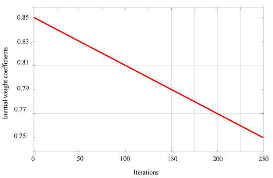
Figure 1.
The relation curve of inertial weight and iterations under linear decreasing.
Linearly decreasing the inertial weight can significantly improve the optimization performance of the particle swarm optimization. However, the particle swarm optimization under a linearly decreasing inertial weight easily falls into the local convergence. Therefore, in the implementation of the particle swarm optimization, a certain amount of constant perturbation is added to make the inertial weight suddenly increase at an iteration, so as to prevent local convergence. The formula of particle swarm optimization adding perturbation constants is described in Equation (6):
where is the initial maximum inertial weight, is the declining slope of the inertial weight. At is the inertial weight perturbation constants, and at the 15% perturbation probability, the At is 0.1; otherwise, At is 0.
The relationship curves for the specific inertial weights and iterations are shown in Figure 2.
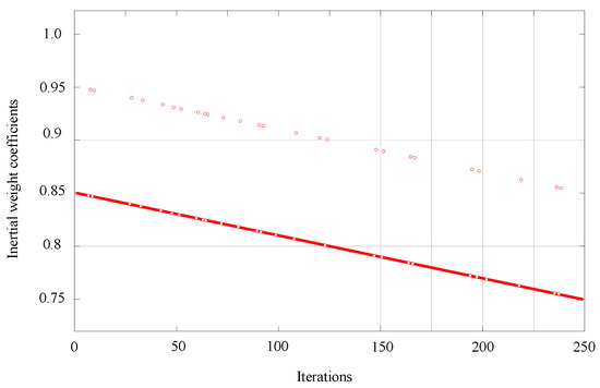
Figure 2.
The relation curve of inertial weight and iterations under linear decreasing with constant perturbation increased.
The following two-point improvement method can be used:
Changing the inertial weight of dynamic adaptation: At 35% probability, the inertial weight obtained by the linear decreasing particle swarm optimization with increasing perturbation is multiplied by a fixed range coefficient r. The coefficient is in the range of 0.8~1.2. The formula is updated as follows:
Random individuals are introduced to maintain the particle population diversity: According to the update of the particle group, the particle swarm optimization brings all individuals close to the optimal particles, resulting in the loss of diversity. A random individual in the solution space is replaced accordingly with the particles obtained by the 25% group algorithm. In general, the introduction of a smaller probability of random individuals does not affect the actual iterative computational trend of the particle swarm optimization.
2.3. Self-Sensing Modeling Based on MPSO LS-SVM
When building a prediction model of the LS-SVM, the selection of the kernel width σ2 and the regularization parameter of kernel function γ determines the performance of the prediction model. Therefore, the prediction and generalization ability of the model can be improved by choosing the appropriate parameters. In order to predict the rotor displacement of magnetic bearing, the MPSO algorithm is used to optimize the parameters σ2 and γ to achieve the optimal prediction effect.
For the six-pole radial HMB, the specific steps for building its prediction model by using the MPSO LS-SVM are shown in Figure 3. The specific process is as follows:
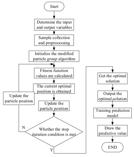
Figure 3.
Flow chart of establishing the model.
- (1)
- Determine the input and output variables of the rotor displacement prediction model for the six-pole radial HMB.
- (2)
- Acquire and preprocess sample data for input and output variables.
- (3)
- Use the MPSO LS-SVM to optimize the performance parameters σ2 and γ. The implementation methods are as follows:
- (a)
- Initialize the parameters. The parameters in the MPSO need to be initialized: population size NP = 20, maximum iteration of the algorithm Tmax = 80, learning factors c1 = c2 = 2, the initial maximum inertial weight = 0.75, and the declining slope of the inertial weight coefficient = 0.001. The initial values of the parameters (σ2, γ) are obtained by initializing the particle swarm at random. The initial displacement prediction model of the magnetic bearings is established by taking the current parameter values as the performance values of LS-SVM when the iteration is 0.
- (b)
- Determine whether the particles meet the requirements. The fitness function of the MPSO algorithm adopts the mean square error of the model prediction value and the actual value, and the expression is as follows:where Np is the total number of training samples, and yi and are the actual value and model predictive value of the rotor displacement.
- (c)
- Update the position and velocity of particles. According to Equation (8), the fitness of each particle is calculated, and the position and velocity of the particle are updated according to Equation (7) to obtain the next-generation particle.
- (d)
- Determine whether or not to terminate the iteration. If the calculated optimal value is less than the preset convergence precision or the current iteration times have reached the preset maximum times, the iteration is stopped, and the result is the output; otherwise, go to step (b) and let t = t + 1.
- (4)
- Obtain the displacement prediction model by training the LS-SVM according to the optimal performance parameters σ2 and γ obtained in step 3.
Therefore, the rotor displacements of the six-pole radial HMB can be predicted by the detected currents so as to achieve the self-sensing of the rotor displacements. In this paper, in order to achieve the best prediction effect, the kernel width σ2 and the regularization parameter γ were optimized using the MPSO and the optimal parameters (σ2, γ) = (1.12, 1200).
3. Simulation Test
3.1. Determine the Input and Output Variables of the Prediction Model
In this six-pole radial HMB, the suspension force is adjusted by changing the control current in the radial control coil, which makes the rotor suspend stably. Therefore, the control currents {ia, ib, ic} are determined as the input variable of the prediction model, and the output variables are the rotor displacements {xb, yb}. Since the LS-SVM used in this paper can only deal with the single-output problem, two prediction models are needed to predict the rotor displacements xb and yb, respectively.
3.2. Data Acquisition and Preprocessing
Obtaining effective sample data is a prerequisite for training the LS-SVM to establish a prediction model. Assuming that the rotor moves at a distance of 0.5 mm near the equilibrium position, take the sinusoidal signal with a frequency of 100 Hz and amplitude value of 0.5 as excitation and collect sample data under the PID closed-loop control system of magnetic bearing; the control currents {ia, ib, ic} form an input sample set, and the rotor displacements {xb, yb} constitute the output sample set. Four hundred sets of data are selected, half of which are randomly selected as training samples to obtain the initial prediction model for offline training of the LS-SVM, and the other half of which are used as test samples to test the prediction accuracy of the prediction model. In order to prevent ill-conditioned data in the calculation process, all the data are processed by the normalized method.
3.3. Model Evaluation
The MPSO and the PSO are compared and analyzed in Matlab. The parameters of the PSO algorithm are set as follows: population quantity Np = 20, termination iterations Tmax = 80, and learning factor c1 = c2 = 2. In the MPSO, the initial maximum inertial weight = 0.75, and the declining slope of the inertial weight coefficient = 0.001.
The fitness curves of the MPSO and PSO are shown in Figure 4. The line with the yellow circle in Figure 4 represents the predicted values of the MPSO, while the line with the black star in Figure 4 represents the predicted values of the PSO. The fitness of the MPSO is obviously smaller than the fitness of the PSO, and the fitness of the MPSO is close to 0 in a short time, but the fitness of the PSO does not stabilize for a long time. This result indicates that the MPSO provides a better predictive performance.
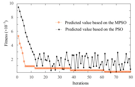
Figure 4.
Mean square error curves of MPSO and PSO.
3.4. Model Prediction Effect
The control diagram of the six-pole hybrid magnetic bearing (SHMB) displacement estimation model is shown in Figure 5. The displacement prediction model turns the control current {ia, ib, ic} to displacement {x, y}. After comparing with the desired displacement {x*, y*}, the displacement {ex, ey} enters the PID controller, and they convert to the desired currents {ix*, iy*}. The desired currents change to the three-phase desired currents {ia*, ib*, ic*}. After comparing the three-phase desired currents with the control current, the SHMB is controlled by the control current output from the three-phase inverter.
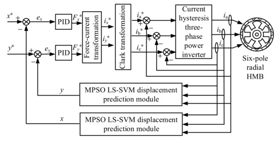
Figure 5.
Control diagram of SHMB displacement estimation system based on MPSO LS-SVM model.
In order to test the prediction ability of the proposed rotor displacement prediction model under different working conditions, according to the displacement estimation method proposed above, the suspension test and anti-interference of Matlab are used to verify the reliability and stability of the six-pole hybrid magnetic bearing without displacement sensor.
The displacement prediction curves of the rotor of the six-pole hybrid magnetic bearing are shown in Figure 6. The rotor suspends from the coordinates (0, −0.5) mm. The black curve shows the actual measured value when the rotor suspends without load; the red curve shows the predicted value based on the MPSO; and the blue curve shows the predicted value based on the PSO. The abscissa is time, and the ordinate is displacement x and y. It can be seen from Figure 6a that the maximum predicted value based on the MPSO in the x direction is −0.37 mm, the maximum predicted value based on the PSO in the x direction is −0.3 m, and the maximum actual measured value in the x direction is −0.38 mm. It can be seen from Figure 6b that the maximum predicted value based on the MPSO in the y direction is 0.18 mm, the maximum predicted value based on the PSO in the y direction is 0.14 mm, and the maximum actual measured value in the y direction is 0.21 mm. The predicted value based on the MPSO is closer to the actual measured value than the predicted value based on the PSO in both the x and y directions; therefore, the prediction ability of the MPSO model is better than the PSO.
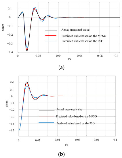
Figure 6.
The displacement prediction curves of the rotor of the six-pole hybrid magnetic bearing: (a) in the x direction; (b) in the y direction.
The displacement prediction curves of the rotor of the six-pole hybrid magnetic bearing when the rotor is disturbed are shown in Figure 7. The rotor suspends from the coordinates (0, −0.5) mm; when the rotor suspends in the equilibrium position, the step signal is added at 0.05 s. It can be seen from Figure 7a that the predicted value based on the PSO in the x direction returns to 0 after 0.03 s, and the predicted value based on the MPSO in the x direction returns to 0 after 0.028 s, which is a reduction of 6.7%. It can be seen from Figure 7b that the predicted value based on the PSO in the y direction returns to 0 after 0.02 s, and the predicted value based on the MPSO in the y direction returns to 0 after 0.016 s, which is a reduction of 20%. The predicted value of the MPSO and the actual measured value are closer. Therefore, the MPSO is more resistant to interference than the PSO.
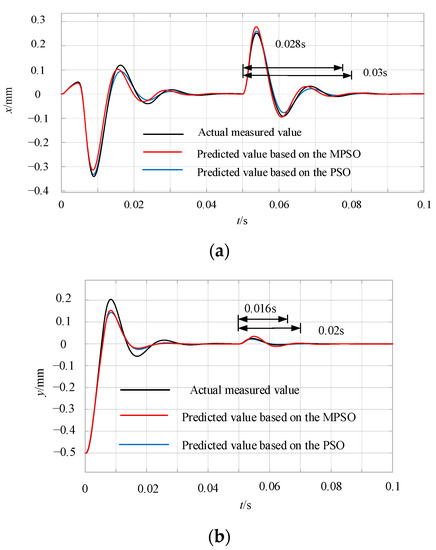
Figure 7.
The displacement prediction curves of the rotor of the six-pole hybrid magnetic bearing when the rotor is disturbed: (a) in the x direction; (b) in the y direction.
4. Experiment Research
In order to verify the accuracy of the above results and further analyze the performance of the six-pole magnetic bearing, an experimental platform was designed and manufactured, as shown in Figure 8. Many experiments are discussed below to demonstrate the robustness and stability of the displacement estimation method. The designed maximum carrying capacity was 220 N, and the parameters of the prototype are shown in Table 1.
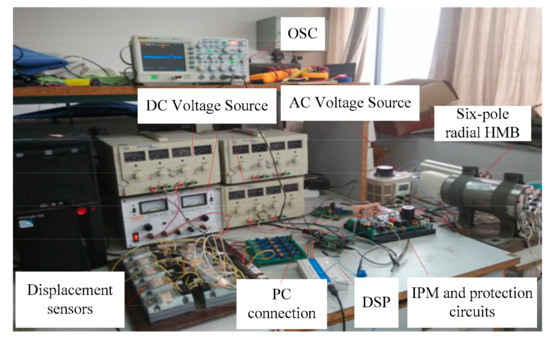
Figure 8.
Experiment platform.

Table 1.
Prototype Parameters.
In this paper, CCS3.3, an integrated development software widely used in DSP, was used to complete the compilation, debugging, and operation of dual-chip radial-axial six-pole HMB. The software VB6.0 was used to develop a man–machine interaction interface and for the online monitoring of experimental data and the online adjustment of the related control parameters. The six-pole radial HMB was driven by an inverter, and the power module used an insulated gate bipolar transistor (IGBT) three-phase full-bridge circuit. The on and off of the six IGBTs changed the amount of current in the three-phase control coil so as to effect adjustments of the rotor position.
Figure 9 shows the suspension experiment of the magnetic bearing: the blue waveform shows the suspension waveform in the x direction; the red waveform shows the suspension waveform in the y direction; the abscissa is the time coordinates, 200 ms per lattice; and the ordinate is the displacement coordinates, 200 μm per lattice. The rotor starts suspension in the fourth grid after about 90 ms. The position of the rotor changes in the x and y directions, stabilizing at the determined position, which is the equilibrium position, indicating that the magnetic bearing can achieve stable suspension in a very short time.
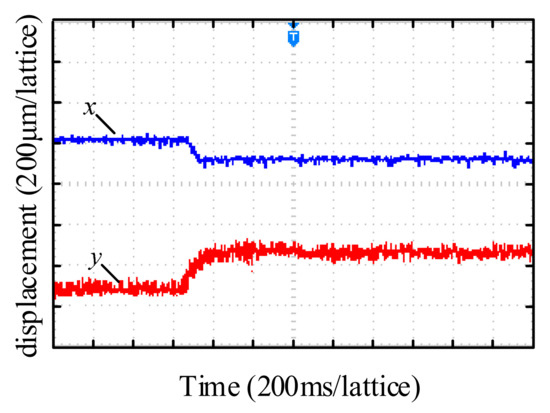
Figure 9.
The waveform of rotor floatation.
Figure 10 shows the suspension experiment at different speeds: the blue waveform shows the displacement waveform in the x direction; the red waveform shows the displacement waveform in the y direction; the abscissa is the time coordinates, 20 ms per lattice; and the ordinate is the displacement coordinates, 200 μm per lattice. To the left of 120 ms, the displacement waveform is shown at 3600 rpm; to the right of 120 ms, the displacement waveform is shown at 1800 rpm. It can be seen from Figure 10 that both the maximum amplitude of the displacement waveform in the x and y directions are 100 μm, which is far shorter than the length of the gas gap. The rotor suspension is stable at different speeds.
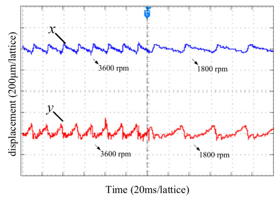
Figure 10.
Rotor displacement at different speeds.
When the system reaches a steady state, a y-direction disturbance is applied to the rotor, and the weight is suspended at one end of the rotor for the purpose of applying a 50 N disturbance power to the rotor. The sample data collected based on the experimental platform is used for model training. The experimental waveforms detected by the PSO prediction model and the MPSO prediction model are shown in Figure 11, where Figure 11a,c indicate the rotor displacement in the x direction, and Figure 11b,d indicate the rotor displacement in the y direction when disturbed. As can be seen from Figure 11, the displacement in the x direction shifts slightly when the rotor in the y direction is disturbed, while the recovery time of the prediction model based on the MPSO is approximately 40 ms shorter than the prediction model based on the PSO, and the rotor displacement offset of the prediction model based on the MPSO is approximately 70 μm less than the prediction model based on the PSO. The experimental results show that the prediction model based on the MPSO has good prediction ability, as well as good anti-interference performance.
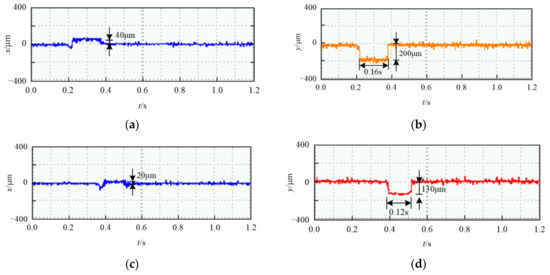
Figure 11.
Displacement waveforms of anti-interference experiment based on the PSO and MPSO. (a) displacement waveform in the x direction of PSO. (b) displacement waveform in the y direction of PSO when disturbed. (c) displacement waveform in the x direction of MPSO. (d) displacement waveform in the y direction of MPSO when disturbed.
Comparing the simulation results of Figure 7 with the experimental results of Figure 11, the experimental results deviate from the simulation results due to rotor gravity and other uncontrollable problems; however, the two verification methods can demonstrate the accuracy of the model and methods proposed in this paper.
5. Conclusions
This manuscript proposes a displacement estimation method using an MPSO LS-SVM. By changing the inertial weight of the MPSO to jump out of the local search and conduct a global search, the optimal parameters are obtained. The simulation results show that the prediction ability of the MPSO model is better than the PSO model and the MPSO model is more resistant to interference than the PSO model. The experiment results show that the magnetic bearing using an MPSO LS-SVM suspends stably in both static and dynamic situations and has good anti-interference capacity and load capacity.
Author Contributions
Conceptualization, G.L. and H.Z.; Data curation, G.L.; Formal analysis, G.L.; Funding acquisition, H.Z.; Investigation, G.L.; Methodology, G.L.; Project administration, H.Z.; Resources, G.L.; Supervision, H.Z.; Validation, G.L.; Visualization, G.L.; Writing—original draft, G.L.; Writing—review & editing, G.L. All authors have read and agreed to the published version of the manuscript.
Funding
This research was funded in part by the National Natural Science Foundation of China, grant number 61973144, and in part by the Priority Academic Program Development of Jiangsu Higher Education Institutions, grant number PAPD-2018-87.
Institutional Review Board Statement
Not applicable.
Informed Consent Statement
Not applicable.
Data Availability Statement
Data is contained within the article.
Conflicts of Interest
The authors declare no conflict of interest.
Nomenclature
| SHMB | Six-pole hybrid magnetic bearing |
| LS-SVM | Least-squares support vector machine |
| MPSO | Modified particle swarm optimization |
| PSO | Particle swarm optimization |
| ia, ib, ic | The input variable of the prediction model |
| xb, yb | The output variable of the prediction model |
| x, y | The rotor position coordinates |
| w | The weight of the LS-SVM |
| b | The bias of the LS-SVM |
| γ | The regularization parameter of the LS-SVM |
| ek | The fitting error of the loss function of the LS-SVM |
| αk | Lagrangian multiplier of the Lagrange function |
| σ | The kernel width of the radial basis kernel function |
| The velocity of the i-th particle of PSO | |
| The position of the i-th particle of PSO | |
| The individual optimal position of PSO | |
| The global optimal position of PSO | |
| c1, c2 | The acceleration constants of PSO |
| rand | The random real number of the interval (0, 1) |
| t | Iterations |
| The inertial weight | |
| The initial maximum inertial weight | |
| The declining slope of the inertial weight | |
| Tmax | The maximum iteration of the algorithm |
| At | The inertial weight perturbation constants |
| r | The fixed range coefficient |
References
- Huang, T.; Zheng, M.; Zhang, G. A Review of Active Magnetic Bearing Control Technology. In Proceedings of the Chinese Control and Decision Conference, CCDC, Nanchang, China, 3–5 June 2019; pp. 2888–2893. [Google Scholar] [CrossRef]
- Gu, H.; Zhu, H.; Hua, Y. Soft Sensing Modeling of Magnetic Suspension Rotor Displacements Based on Continuous Hidden Markov Model. IEEE Trans. Appl. Supercond. 2017, 28, 1–5. [Google Scholar] [CrossRef]
- Le, Y.; Wang, K. Design and Optimization Method of Magnetic Bearing for High-Speed Motor Considering Eddy Current Effects. IEEE/ASME Trans. Mechatron. 2016, 21, 2061–2072. [Google Scholar] [CrossRef]
- Usman, I.; Paone, M.; Smeds, K.; Lu, X. Radially Biased Axial Magnetic Bearings/Motors for Precision Rotary-Axial Spindles. IEEE/ASME Trans. Mechatron. 2011, 16, 411–420. [Google Scholar] [CrossRef]
- Abooee, A.; Arefi, M. Robust finite-time stabilizers for five-degree-of-freedom active magnetic bearing system. J. Frankl. Inst.-Eng. Appl. Math. 2019, 356, 80–102. [Google Scholar] [CrossRef]
- Zhang, W.; Zhu, H.; Yang, Z.; Sun, X.; Yuan, Y. Nonlinear model analysis and “switching model” of AC–DC three degree of freedom hybrid magnetic bearing. IEEE/ASME Trans. Mechatron. 2016, 21, 1102–1115. [Google Scholar] [CrossRef]
- Zhang, W.; Yang, H.; Cheng, L.; Zhu, H. Modeling Based on Exact Segmentation of Magnetic Field for a Centripetal Force Type-Magnetic Bearing. IEEE Trans. Ind. Electron. 2019, 67, 7691–7701. [Google Scholar] [CrossRef]
- Wang, S.; Zhu, H.; Wu, M.; Zhang, W. Active Disturbance Rejection Decoupling Control for Three-Degree-of-Freedom Six-Pole Active Magnetic Bearing Based on BP Neural Network. IEEE Trans. Appl. Supercond. 2020, 30, 1–5. [Google Scholar] [CrossRef]
- Liu, G.; Zhu, H.; Zhang, W. Principle and performance analysis for six-pole hybrid magnetic bearing with a secondary air gap. Electron. Lett. 2021, 57, 548–549. [Google Scholar] [CrossRef]
- Ernst, D.; Faghih, M.; Liebfried, R.; Melzer, M.; Karnaushenko, D.; Hofmann, W.; Schmidt, O.G.; Zerna, T. Packaging of Ultrathin Flexible Magnetic Field Sensors With Polyimide Interposer and Integration in an Active Magnetic Bearing. IEEE Trans. Components, Packag. Manuf. Technol. 2020, 10, 39–43. [Google Scholar] [CrossRef]
- Zhu, Z.; Dai, M.; Zeng, L.; Sun, J.; Zhang, Y. Research on testing principle of self-sensing magnetic bearing system. 2018 4th International Conference on Control, Automation and Robotics (ICCAR), Auckland, New Zealand, 20–23 April 2018; 2018; pp. 301–304. [Google Scholar] [CrossRef]
- Tera, T.; Yamauchi, Y.; Chiba, A.; Fukao, T.; Rahman, M. Performances of bearingless and sensorless induction motor drive based on mutual inductances and rotor displacements estimation. IEEE Trans. Ind. Electron. 2006, 53, 187–194. [Google Scholar] [CrossRef]
- Haarnoja, T.; Tammi, K.; Manninen, A.; Halmeaho, T. Position estimation method for self-sensing electric machines based on the direct measurement of the current slope. IET 2014. [Google Scholar] [CrossRef]
- Yim, J.-S.; Sul, S.-K.; Ahn, H.-J.; Han, D.-C. Sensorless position control of active magnetic bearings based on high frequency signal injection with digital signal processing. IEEE 2004, 2, 1351–1354. [Google Scholar] [CrossRef]
- Hofer, M.; Schmidt, E.; Schrodl, M. Design of a Three Phase Permanent Magnet Biased Radial Active Magnetic Bearing Regarding a Position Sensorless Control. In 2009 Twenty-Fourth Annual IEEE Applied Power Electronics Conference and Exposition; IEEE: Piscataway, NJ, USA, 2009; pp. 1716–1721. [Google Scholar] [CrossRef]
- García, P.; Guerrero, J.M.; Briz, F.; Reigosa, D.D. Sensorless Control of Three-Pole Active Magnetic Bearings Using Saliency-Tracking-Based Methods. IEEE Trans. Ind. Appl. 2010, 46, 1476–1484. [Google Scholar] [CrossRef]
- Sun, Z.; Zhao, J.; Shi, Z.; Yu, S. Soft sensing of magnetic bearing system based on support vector regression and extended Kalman filter. Mechatronics 2014, 24, 186–197. [Google Scholar] [CrossRef]
- Xu, B.; Zhang, L.; Ji, W. Improved Non-Singular Fast Terminal Sliding Mode Control With Disturbance Observer for PMSM Drives. IEEE Trans. Transp. Electrif. 2021, 7, 2753–2762. [Google Scholar] [CrossRef]
- Chen, S.; Hung, Y.; Hung, Y. Application of a recurrent wavelet fuzzy-neural network in the positioning control of a magnetic-bearing mechanism. Comput. Electric. Engineering 2015, 54, 147–158. [Google Scholar] [CrossRef]
- Suykens, J.; Vandewalle, J. Recurrent least squares support vector machines. IEEE Trans. Circuits Syst. I Regul. Pap. 2000, 47, 1109–1114. [Google Scholar] [CrossRef]
- Sun, Y.; Zhu, Z. Inverse-model identification and decoupling control based on least squares support vector machine for 3-degree-of-freedom hybrid magnetic bearing. Proc. CSEE 2010, 30, 112–117. [Google Scholar]
- Jin, J.; Zhu, H.Q. Technique for Magnetic Bearing Based on Mixed-Kernel Support Vector Machine Forecasting Model. Appl. Mech. Mater. 2014, 529, 349–353. [Google Scholar] [CrossRef]
Publisher’s Note: MDPI stays neutral with regard to jurisdictional claims in published maps and institutional affiliations. |
© 2022 by the authors. Licensee MDPI, Basel, Switzerland. This article is an open access article distributed under the terms and conditions of the Creative Commons Attribution (CC BY) license (https://creativecommons.org/licenses/by/4.0/).