Two-Stage Robust Economic Dispatch of Regional Integrated Energy System Considering Source-Load Uncertainty Based on Carbon Neutral Vision

Abstract

A regional integrated energy system is an important carrier of the energy Internet. It is a major challenge for the operation of a regional integrated energy system to deal with the uncertainty of distributed energy and multiple loads by using the coupling characteristics of equipment in a regional integrated energy system. In this paper, a two-stage robust economic dispatch model of a regional integrated energy system is proposed considering the source-load uncertainty. Firstly, the basic architecture of the regional integrated energy system is introduced. Based on the extreme scenario of uncertain power supply and load, the uncertainty set was established, the two-stage robust optimization model of regional integrated energy system was constructed and the column-and-constraint generation algorithm was used to solve the model. The effectiveness of the two-stage robust optimization model in improving the economy and robustness of the system was analyzed.

1. Introduction

China proposes to achieve the development goal of carbon neutrality by 2060 to contribute to the sustainable economic development of the Asia-Pacific region [1]. To achieve this, renewable energy penetration must be increased. However, with the increase in the penetration rate of renewable energy, large-scale renewable energy is difficult to absorb, and the phenomenon of “abandoning wind and light” still exists. With the increase in energy consumption, the failure of the power grid often endangers other energy systems. The problem of independent planning and operation of renewable energy and various energy systems is becoming increasingly prominent. Faced with this challenge, the concept of the energy Internet has emerged and become the focus of academic and industrial circles [2]. The outstanding feature of the energy Internet is the combination of new energy technology and information technology, and the complementary coupling of cold, heat and electricity energy. According to the scale, integrated energy systems can be divided into trans-regional level, regional level and user level [3]. A regional integrated energy system (RIES) is the manifestation of regional distribution and system characteristics of an integrated energy system. The RIES is involved in energy production, conversion, transportation, storage and use; the depth of fusion power, intermittent renewable energy sources such as wind, solar, natural gas, biomass energy and environmental energy, such as thermal energy through various types of complementary energy between coupling and optimization, and renewable energy in order to meet the user’s cold, heat, electricity and other energy demand. At the same time, efficient and clean utilization of energy can be achieved [4,5,6].

How to utilize the multi-energy coupling of RIESs and the flexibility of multi-type energy storage to cope with the uncertainty of electricity, gas and heat loads and renewable energy is a frequently studied topic in the research of integrated energy systems, as is research on regional integrated energy [7,8,9,10]. Ref. [7] discussed the transformation of regional integrated energy with the control of carbon emission reduction, and took Dalian City, China, as an example for analysis. Ref. [9] studied the market transaction and management of regional integrated energy considering the application of high proportion of renewable energy.

Ref. [11] considers that the use of battery energy storage systems (BESSs) as backup power affects the operating costs of regional integrated energy systems (RIESs) in different situations and describes a regional integrated energy system that includes wind turbines, photovoltaic generators, gas turbines and battery energy storage systems. Refs. [8,12] proposes a multi-objective stochastic programming method based on the generation method of multi-dimensional associated scenario sets for RIES expansion plans. The scenario generation method considers the characteristics, timing, autocorrelation and cross-correlation of renewable energy and multi-energy loads. Considering the importance of the energy pipeline, the pipeline risk index of energy network expansion planning is defined. Meanwhile, a multi-objective stochastic energy network-based opportunity-constrained programming model is proposed to reduce investment costs and pipeline risks. Ref. [13] extended the concept of demand response (DR) to the RIES and proposed an optimized operation model of the RIES considering the DR mechanism on energy prices. Based on the DR modeling of the RIES, the operation optimization model with environmental benefits, economic benefits and energy supply reliability as objective functions was established in detail for the first time. In the configuration of the rated capacity and power of various energy storage devices in the RIES [14], off-grid and grid-connected operation modes are proposed and a configuration optimization model is established. The RIES is divided into four parts: power supply, energy conversion, energy storage and load. Based on the concept of the energy hub, the four parts are modeled separately.

However, it is difficult to obtain the probability distribution of random parameters in practical application, which limits the application of the above reference algorithm. The global optimality of solution efficiency and solution cannot be satisfied simultaneously because of the existence of non-convex constraints in chance-constrained programming. The computational efficiency and accuracy of the probabilistic scenario method are easily affected by the number of generated scenarios and the method of scene generation and reduction.

Robust optimization does not require presupposition of the distribution followed by uncertain parameters. After the fluctuation range of the uncertain parameters is determined in advance, when the value of the uncertain parameters falls in the given uncertain set, the constraints of the robust optimization model must be satisfied, and the deterministic feasible solution [15,16,17] can be obtained. Robust optimization has developed into an important and very common tool to deal with uncertain optimization problems and has been widely used in power system optimization scheduling [18,19,20,21,22,23,24]. In view of the existence of various uncertainties, Ref. [23] proposed an uncertainty quantification method for energy management. In the rescheduling stage, decision variables representing the charge and discharge state of energy storage systems were considered, while the existing model places them in the pre-scheduling stage to improve the operational flexibility of energy storage systems in energy management.

Two-stage robust optimization (TRO) can ensure the normal operation of the system in the most extreme case where only the fluctuation range information of uncertain parameters is obtained. At the same time, TRO can adjust the conservatism of the system through dynamic iteration strategy. This addresses the deficiency of the traditional robust optimization method.

The contributions of this study can be summarized as follows.

(1)

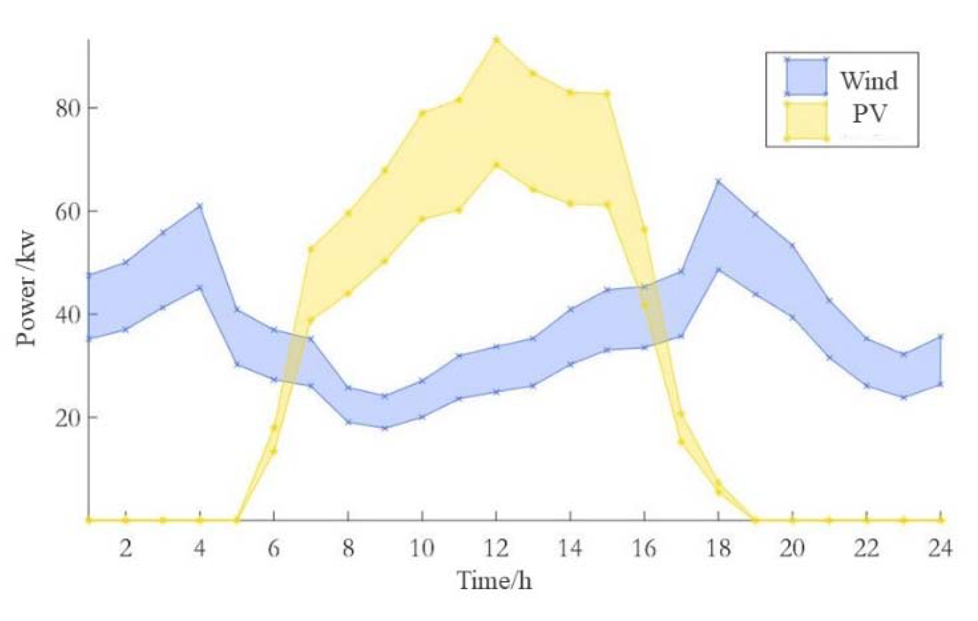
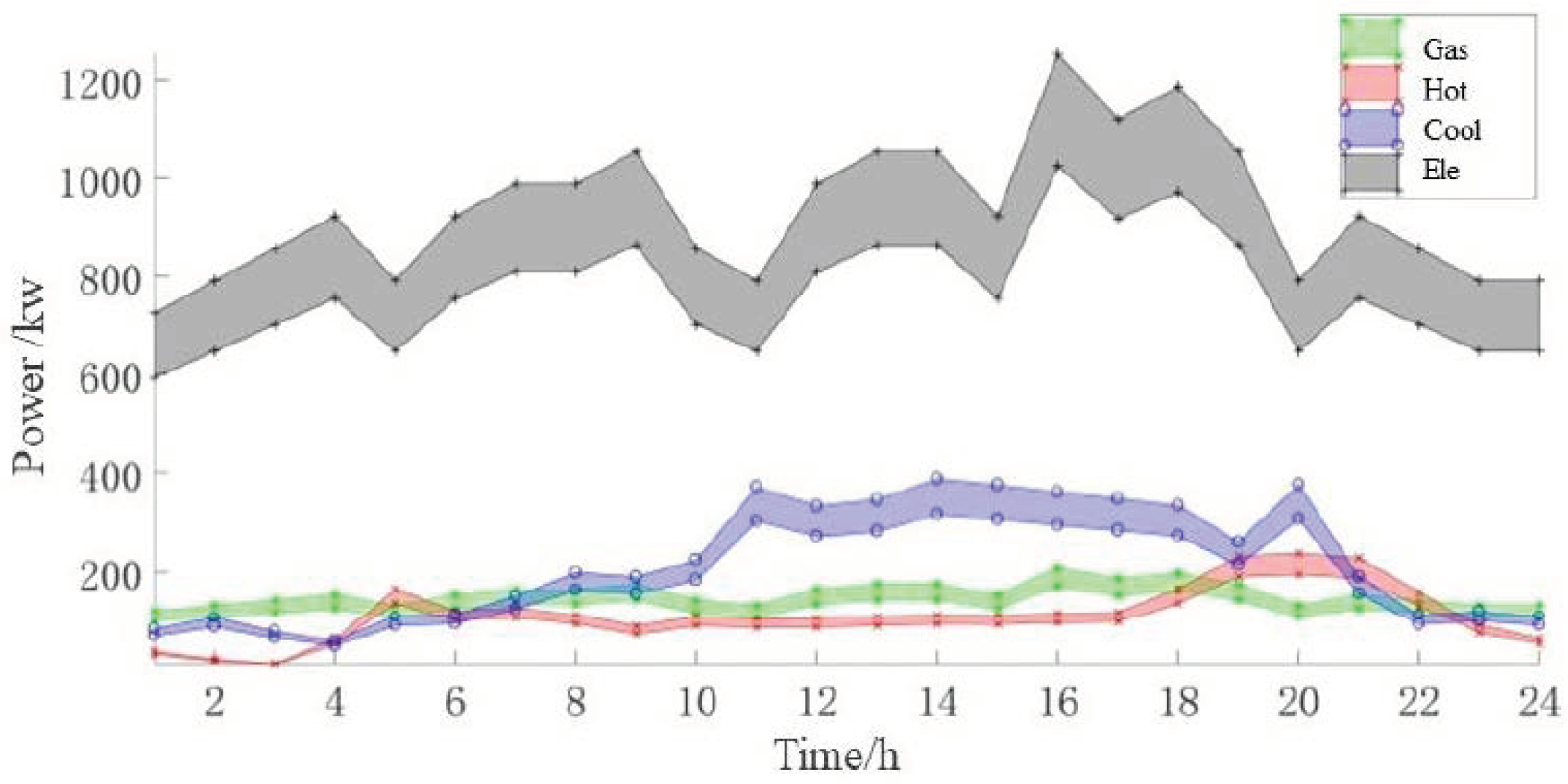
The uncertainties of wind power, photovoltaic output and multiple types of loads were considered, and a two-stage robust and optimized economic scheduling model was established with the goal of minimizing operation cost and regulation cost with day-ahead scheduling. First, the model was built taking into account the electrical, gas and thermal network characteristics of the RIES as well as energy conversion equipment, energy storage equipment and various composite characteristics. Considering the extreme cases of wind and photovoltaic power and load forecasting errors in day-ahead scheduling, the TRO model was constructed.

(2)

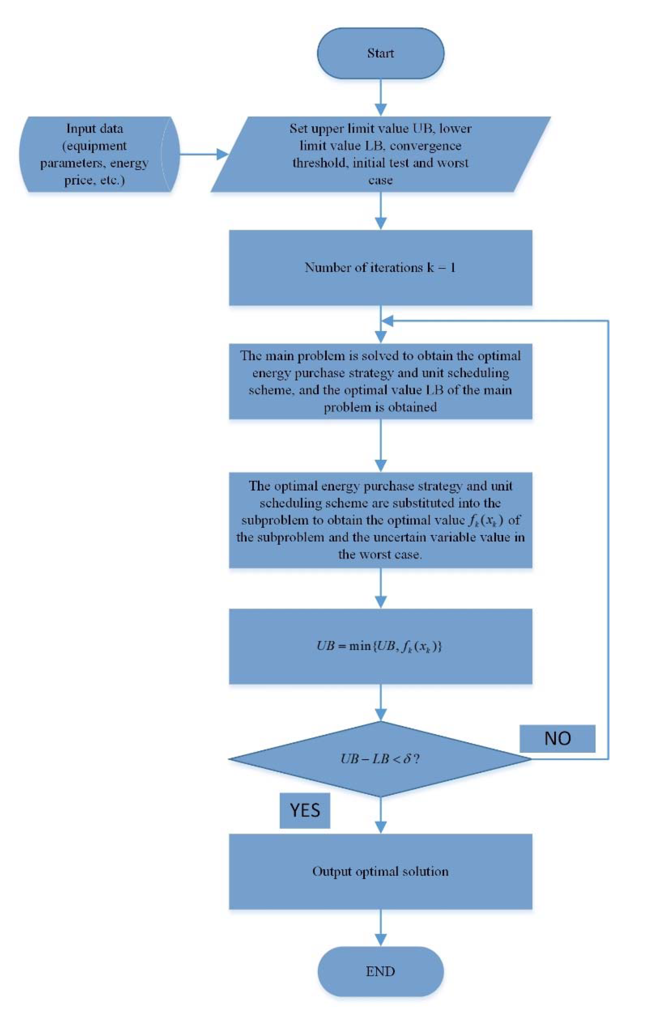
Combined with the strong duality theory, the column-and-constraint generation algorithm was used to transform the model into a mixed integer linear programming problem.

(3)

A regional integrated energy system in summer was taken as an example to verify the effectiveness of the model. The difference between the two-stage robust optimization model with the deterministic scheduling method and the worst case with different uncertain budget values was compared and analyzed. The results show that the two-stage robust economic optimization model can significantly improve the operating economy of the system.

The remainder of this paper is organized as follows. In Section 2, the structural framework of the regional integrated energy system is introduced. Section 3 mainly lists the output model of the main equipment of the regional integrated energy system. In Section 4, the construction of a two-stage robust optimal scheduling model is detailed, the objective function is proposed to minimize the system adjustment cost and the constraints of the system are listed. Section 5 proposes column-and-constraint generation to solve the model. In Section 6, a case study is outlined to prove the validity and economy of the proposed model. Concluding remarks are given in Section 7.

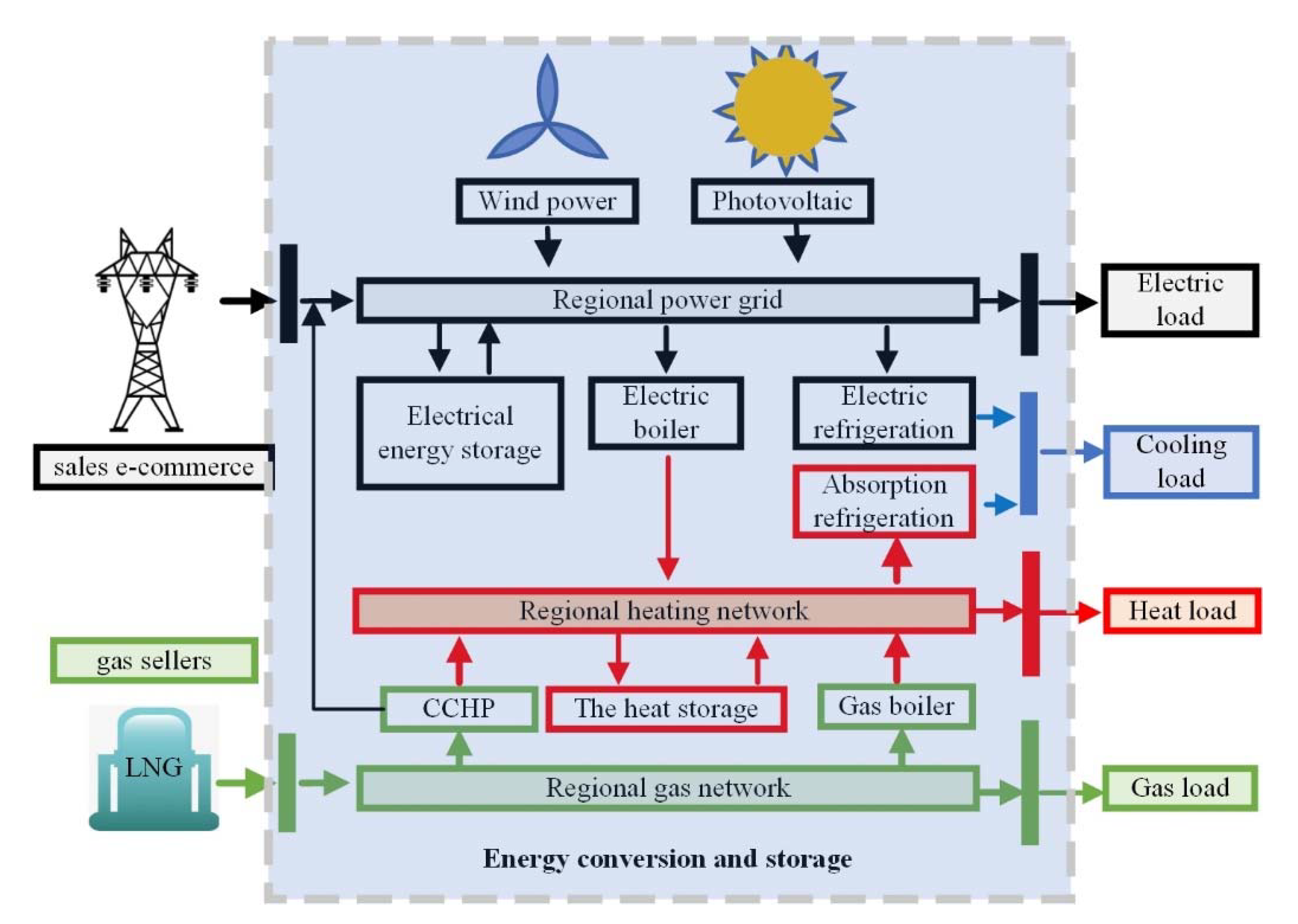
2. Regional Integrated Energy System Structure

In structure, a RIES can be regarded as an energy unit with multiple inputs, outputs, conversions and storage devices. Based on common forms of regional integrated energy systems, a RIES containing energy coupling units, distributed power sources and energy storage devices was constructed. The structure of the RIES is shown in Figure 1. The energy coupling unit includes the gas turbine cogeneration unit, gas boiler, electric boiler, electric refrigeration equipment and absorption refrigeration equipment. Distributed power includes distributed wind power and distributed photovoltaic power generation units. Energy storage equipment includes electric energy storage and thermal energy storage. The RIES purchases online energy from the upstream external power grid and heat network and natural gas through the regional electricity, heat and gas vendors. The energy is reasonably distributed through conversion and storage devices to meet various needs of users.

3. Regional Integrated Energy System Main Equipment Model

3.1. GAS Turbine Cogeneration Unit

GAS Turbine Cogeneration Unit is an important part of regional Integrated Energy system.

$$P_t^{GT}={\eta }_{}^{GT,p}{\alpha }_t^{GT,p}{G}_t^{GT}$$

(1)

$$P_{}^{GT,\min }\le P_t^{GT}\le P_{}^{GT,\max }$$

(2)

$$H_t^{GT}={\eta }_{}^{GT,h}(1-{\alpha }_p^{GT})G_t^{GT}$$

(3)

$$H_{}^{GT,\min }\le H_t^{GT}\le H_{}^{GT,\max }$$

(4)

where $P_t^{GT}$ and $H_t^{GT}$ are the electrical power and thermal power output by the gas turbine at time period $t$, respectively; $G_t^{GT}$ is the amount of natural gas consumed by gas turbine in time period $t$; ${\eta }_{}^{GT,p}$ is the power generation efficiency of gas turbine; ${\eta }_{}^{GT,h}$ is the waste heat recovery efficiency of gas turbine; ${\alpha }_t^{GT,p}$ is the scheduling factor of gas turbine in time period $t$; $P_{}^{GT,\min }$ and $P_{}^{GT,\max }$ are the minimum and maximum output power of gas turbine, respectively; $H_{}^{GT,\min }$ and $H_{}^{GT,\max }$ are the minimum and maximum thermal output power of gas turbine, respectively.

3.2. Gas Boiler

When the heat energy recovered by waste heat recovery device cannot meet the demand of the heat load, gas-fired boiler can be used to supply energy to part of the heat load. The thermal power output constraint of the gas-fired boiler can be expressed as follows.

$$H_t^{GB}={\eta }_{}^{GB}{G}_t^{GB}$$

(5)

$$H_{}^{GB,\min }\le H_t^{GB}\le H_{}^{GB,\max }$$

(6)

where $H_t^{GB}$ is the thermal power output by gas boiler in time period $t$; $G_t^{GB}$ is the amount of natural gas consumed by gas boiler in time period $t$ and ${\eta }_{}^{GB}$ is the heating efficiency of gas boiler. $H_{}^{GB,\min }$ and $H_{}^{GB,\max }$ are the minimum and maximum thermal power of the gas-fired boiler, respectively.

3.3. Electric Boiler

The power constraints of electric heating boilers are shown below.

$$H_t^{EB}={\eta }_{}^{EB}{P}_t^{EB}$$

(7)

$$H_t^{EB,\min }\le H_t^{EB}\le H_t^{EB,\max }$$

(8)

where $H_t^{EB}$ is the thermal power output by the electric boiler in time period $t$; $P_t^{EB}$ is the amount of natural gas consumed by the electric boiler in time period $t$ and ${\eta }_{}^{EB}$ is the power generation efficiency of the electric boiler; $H_{}^{GB,\min }$ and $H_{}^{GB,\max }$ are the minimum and maximum thermal power of electric boiler, respectively.

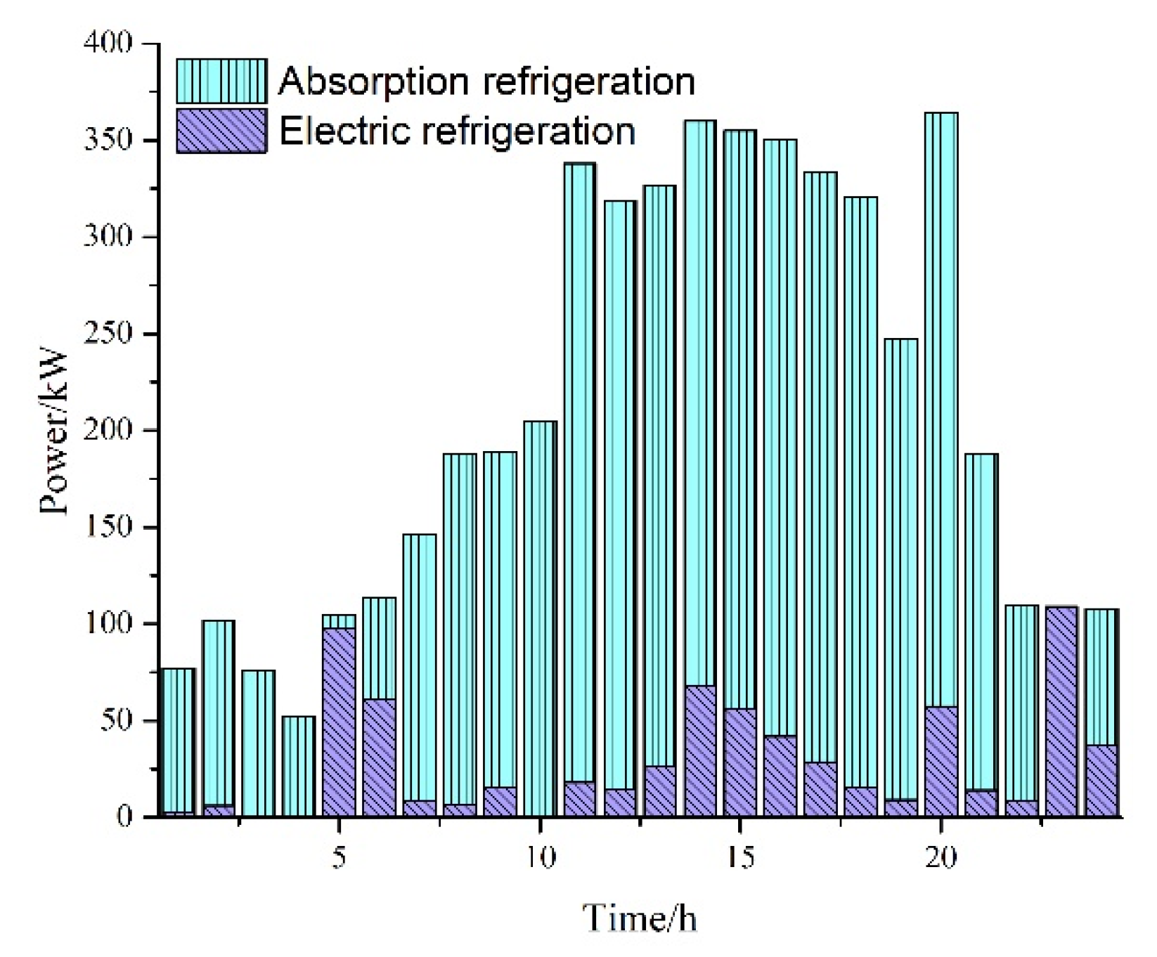
3.4. Absorption Refrigeration

Absorption chillers use thermal energy to drive the refrigeration cycle and consume thermal energy for refrigeration. The power constraints of an absorption chiller are described as follows.

$$C_t^{AC}={\eta }_{}^{AC}{H}_t^{AC}$$

(9)

$$C_{}^{AC,\min }\le C_t^{AC}\le C_{}^{AC,\max }$$

(10)

where $C_t^{AC}$ is the output power of the absorption chiller in time period $t$, $H_t^{AC}$ is the thermal power absorbed by the absorption chiller in time period $t$, ${\eta }_{}^{AC}$ is the efficiency of heat exchange device, $C_{}^{AC,\min }$ and $C_{}^{AC,\max }$ are the maximum and minimum output power of the absorption chiller, respectively.

3.5. Electric Refrigeration

The physical model of an electric refrigerator is described as follows:

$$C_t^{EC}={\eta }_{}^{EC}{P}_t^{EC}$$

(11)

$$C_{}^{EC,\min }\le C_t^{EC}\le C_{}^{EC,\max }$$

(12)

where $C_t^{EC}$ is the output power of the electric refrigerator in time period $t$, $P_t^{EC}$ is the thermal power absorbed by the electric refrigerator in time period $t$, ${\eta }_{}^{EC}$ is the conversion efficiency of the electric refrigerator, $C_{}^{EC,\min }$ and $C_{}^{EC,\max }$ are the maximum and minimum output power of the electric refrigerator, respectively.

3.6. Heat Storage Equipment

The heat storage device can store heat and release heat when the system heat is insufficient. It is assumed that there is no energy dissipation over time in the heat storage device, and the energy storage model of the heat storage device can be expressed as:

$$u_t^{HS,ch}{H}_{}^{HS,ch,\min }\le H_t^{HS,ch}\le u_t^{HS,ch}{H}_t^{HS,ch,\max }$$

(13)

$$u_t^{HS,dis}{H}_{}^{HS,dis,\min }\le H_t^{HS,dis}\le u_t^{HS,dis}{H}_t^{HS,dis,\max }$$

(14)

$$S_{}^{H,\min }\le S_t^H\le S_{}^{H,\max }$$

(15)

$$S_{t+1}^H=S_t^H+({\eta }_{}^{HS,ch}{H}_t^{HS,ch}-H_t^{HS,dis}/{\eta }_{}^{HS,dis})/Ca{p}_{}^{HS}$$

(16)

$$S_0^H=S_T^H$$

(17)

$$u_t^{HS,ch}+u_t^{HS,dis}\le 1$$

(18)

where $H_t^{HS,ch}$ and $H_t^{HS,dis}$ are respectively the heat storage and release power of the heat storage device at time period $t$; $H_{}^{HS,ch,\min }$ and $H_{}^{HS,ch,\max }$ are the minimum and maximum heat storage power of the heat storage device, respectively; $H_{}^{HS,dis,\min }$ and $H_{}^{HS,dis,\max }$ are the minimum and maximum heat release powers of the heat storage device, respectively; $u_t^{HS,ch}$ and $u_t^{HS,dis}$ are the storage and heat release state variables of the heat storage device in time period $t$, respectively; $S_t^H$ is the state of heat storage capacity of heat storage device in time period $t$; $S_{}^{H,\min }$ and $S_{}^{H,\max }$ are the minimum and maximum heat storage capacity of the heat storage device, respectively; ${\eta }_{}^{HS,ch}$ and ${\eta }_{}^{HS,dis}$ correspond to the heat storage and heat release efficiency of the heat storage device, respectively. $Ca{p}_{}^{HS}$ is the rated capacity of the heat storage device.

3.7. Electric Energy Storage

The electrical storage device can store energy during the RIES distributed power supply peak and off-load periods and discharge energy during the RIES distributed power supply with output or peak consumption periods. The electric energy storage device model can be expressed as:

$$u_t^{ES,ch}{P}_{}^{ES,ch,\min }\le P_t^{ES,ch}\le u_t^{ES,ch}{P}_t^{ES,ch,\max }$$

(19)

$$u_t^{ES,dis}{P}_{}^{ES,dis,\min }\le P_t^{ES,dis}\le u_t^{ES,dis}{P}_t^{ES,dis,\max }$$

(20)

$$S_{}^{E,\min }\le S_t^E\le S_{}^{E,\max }$$

(21)

$$S_{t+1}^E=S_t^E+({\eta }_{}^{ES,ch}{P}_t^{ES,ch}-P_t^{ES,dis}/{\eta }_{}^{ES,dis})/Ca{p}_{}^{ES}$$

(22)

$$S_0^E=S_T^E$$

(23)

$$u_t^{ES,ch}+u_t^{ES,dis}\le 1$$

(24)

where $P_t^{ES,ch}$ and $P_t^{ES,dis}$ are respectively the charge and discharge power of electric energy storage equipment in time period $t$; $P_{}^{ES,ch,\min }$ and $P_{}^{ES,ch,\max }$ are the minimum and maximum charging power of electric energy storage equipment, respectively; $P_{}^{ES,dis,\min }$ and $P_{}^{ES,dis,\max }$ are the minimum and maximum discharge power of electric energy storage equipment, respectively; $u_t^{ES,ch}$ and $u_t^{ES,dis}$ are charge and discharge state variables of the electric energy storage device at time period $t$, respectively; $S_t^E$ is the charged state of the electric energy storage device at time period $t$; $S_{}^{E,\min }$ and $S_{}^{E,\max }$ are the minimum and maximum state of charge of electric energy storage equipment, respectively. ${\eta }_{}^{ES,ch}$ and ${\eta }_{}^{ES,dis}$ respectively refer to the charging and discharging efficiency of an electric energy storage device; $Ca{p}_{}^{ES}$ is the rated capacity of an electric energy storage device.

3.8. Modeling of Uncertainties

Considering the actual output of distributed power sources such as distributed wind power and distributed photovoltaic power, and that all kinds of user loads such as cold, heat, gas and electricity fluctuate around the predicted output, in this study, the uncertainty sets of distributed power supply and multi-class load were established to describe the related uncertainties, and a two-stage robust optimal scheduling model of integrated energy was established.

This study analyzed the historical data of wind power and photovoltaic output. According to the historical data, a range was selected to cover all wind power or photovoltaic output scenarios in a given period of time. Thus, the uncertain performance of wind and photovoltaic power can be expressed as follows with the uncertainty set constrained by a certain radius:

$$U^x=\{{\tilde{P}}_t^x=({\tilde{P}}_1^x,{\tilde{P}}_2^x,\cdots ,{\tilde{P}}_T^x,)\}$$

(25)

$${\tilde{P}}_t^x=P_t^{x,f}+z_t^{x,1+}{\overline{P}}_t^x-z_t^{x,1-}{\underset{\_}{P}}_t^x$$

(26)

$${\displaystyle \sum _{t=1}^T(z_t^{x,1+}+z_t^{x,1-})\le {\Gamma }^x}$$

(27)

$$z_t^{x,1+}+z_t^{x,1-}\le 1$$

(28)

where $U^x$ refers to the uncertain set of wind and photovoltaic power and user load such as cold, heat, gas and electricity; $x\in \{W,PV,HL,CL,GL,PL\}$ is energy and load type. ${\tilde{P}}_t^x$ represents uncertain variables in the system; $P_t^{x,f}$ represents the predicted value of distributed power and load. ${\overline{P}}_t^x$ and ${\underset{\_}{P}}_t^x$ represent the upper and lower limits of fluctuation deviation of distributed power supply and load, respectively; $z_t^{x,1+}$ and $z_t^{x,1-}$ are auxiliary 0–1 variables describing the distributed power supply and the actual load value at the upper or lower boundary. ${\Gamma }^x$ is the uncertain budget value, which is used to adjust the conservatism of the optimal solution; the larger its value, the more conservative the final scheduling scheme.

4. Regional Integrated Energy System Two-Stage Robust Optimal Scheduling Model Considering Bilateral Uncertainties

Based on the RIES model, a two-stage robust optimization RIES model was established. The first phase aims to determine the optimal scheduling scheme for wind, photovoltaic and multi-energy loads in the day-ahead forecast scenario. Based on the optimization results of the first stage, the output of each unit is adjusted again in the second stage to cope with the “most extreme” scenario with the largest prediction error with the day-ahead scheduling scheme, and the results are fed back to the first stage. Through the iterations of the first and second stages, all extreme scenarios can satisfy the given constraints, and the corresponding day-ahead scheduling strategy can be obtained.

4.1. The Objective Function

A two-stage robust optimization RIES model is presented in this paper, and the objective function is shown in Equations (29)–(32). The main objective of the first stage is to minimize the total energy consumption cost and operation and maintenance cost of the RIES with the given day-ahead forecast, and the max–min objective of the second stage ensures the lowest system adjustment cost in the uncertain scenario of intra-day scheduling.

$$Obj=\underset{x}{\min }(F_f+F_o)+\underset{u}{\max }\underset{y}{\min }{F}_{\Delta }$$

(29)

$$F_f={\displaystyle \sum _{t=1}^T{a}_t^{b,gas}{G}_t^b+a_t^{b,ele}{P}_t^b}$$

(30)

$$\begin{array}{ll}{F}_o=& {\displaystyle \sum _{t=1}^T(a_t^{GT,P}{P}_t^{GT}+a_t^{GT,H}{H}_t^{GT}+a_t^{GB}{H}_t^{GB}}\\ & +a_t^{EB}{H}_t^{EB}+a_t^{AC}{C}_t^{AC}+a_t^{EC}{C}_t^{EC}\\ & +a_t^{HS}(H_t^{HS,ch}+H_t^{HS,dis})\\ & +a_t^{ES}(P_t^{ES,ch}+P_t^{ES,dis})\\ & +a_t^{W,cut}{P}_t^{W,cut}+a_t^{PV,cut}{P}_t^{PV,cut})\end{array}$$

(31)

$$\begin{array}{ll}{F}_{\Delta }=& {\displaystyle \sum _{t=1}^T(b_t^G\Delta G_t^b+b_t^P\Delta P_t^b+b_t^{GT,P}\Delta P_t^{GT}}\\ & +b_t^{GT,H}\Delta H_t^{GT}+b_t^{GB}\Delta H_t^{GB}\\ & +b_t^{EB}\Delta H_t^{EB}+b_t^{AC}\Delta C_t^{AC}\\ & +b_t^{EC}\Delta C_t^{EC}+b_t^{HS}(\Delta H_t^{HS,ch}\\ & -\Delta H_t^{HS,dis})+b_t^{ES}(\Delta P_t^{ES,ch}\\ & -\Delta P_t^{ES,dis})+b_t^{W,cut}\Delta P_t^{W,cut}\\ & +b_t^{PV,cut}\Delta P_t^{PV,cut})\end{array}$$

(32)

where $\Delta •$ represents the deviation of each scheduling value in intra-day scheduling relative to intra-day scheduling; $b_t^{•}$ represents the penalty cost of unit deviation of each conversion equipment and purchased energy.

4.2. The Constraints

Constraints are divided into first-stage constraints and second-stage constraints. The first-stage constraints include energy network and coupling device constraints in the day-ahead scheduling process. The second stage constraints include the adjustment constraints of electricity, gas, heat networks and coupling equipment with the uncertain parameters of the day.

4.2.1. First Stage Constraints

The constraints in the first stage include Equations (1)–(24), discarding wind discard light constraint (33)–(34) and power balance constraints in the prediction scenario, as shown in (35)–(38).

$$0\le P_t^{W,cut}\le P_t^{W,f}$$

(33)

$$0\le P_t^{PV,cut}\le P_t^{PV,f}$$

(34)

$$G_t^b=L_t^{g,f}+G_t^{GT}+G_t^{GB}$$

(35)

$$C_t^{AC}+C_t^{EC}=L_t^{c,f}$$

(36)

$$H_t^{GT}+H_t^{GB}+H_t^{EB}+H_t^{HS,dis}=L_t^{H,f}+H_t^{AC}+H_t^{HS,ch}$$

(37)

$$P_t^b+P_t^{GT}+P_t^{ES,dis}+P_t^{W,f}+P_t^{PV,f}=L_t^{ele,f}+P_t^{EB}+P_t^{EC}+P_t^{ES,ch}$$

(38)

where $P_t^{W,cut}$ and $P_t^{PV,cut}$ represent the amount of wind and light abandoning in time period $t$, respectively; $P_t^{W,f}$ and $P_t^{PV,f}$ represent the predicted output values of wind and photovoltaic power in time period $t$, respectively.

4.2.2. Second Stage Constraints

Because the constraint of the first stage does not consider the influence of the uncertain scenario in the real-time operation stage, in the second stage, distributed power supply and multiple types of loads are introduced into the constraints, and rescheduling constraints in uncertain scenarios are considered in the day-ahead scheduling of the RIES. The second-stage constraints are shown below.

$$P_{}^{GT,\min }\le P_t^{GT}+\Delta P_t^{GT}\le P_{}^{GT,\max }$$

(39)

$$H_{}^{GT,\min }\le H_t^{GT}+\Delta H_t^{GT}\le H_{}^{GT,\max }$$

(40)

$$H_{}^{GB,\min }\le H_t^{GB}+\Delta H_t^{GB}\le H_{}^{GB,\max }$$

(41)

$$H_t^{EB,\min }\le H_t^{EB}+\Delta H_t^{EB}\le H_t^{EB,\max }$$

(42)

$$C_{}^{AC,\min }\le C_t^{AC}+\Delta C_t^{AC}\le C_{}^{AC,\max }$$

(43)

$$C_{}^{EC,\min }\le C_t^{EC}+\Delta C_t^{EC}\le C_{}^{EC,\max }$$

(44)

$$u_t^{HS,ch}{H}_{}^{HS,ch,\min }\le H_t^{HS,ch}+\Delta H_t^{HS,ch}\le u_t^{HS,ch}{H}_t^{HS,ch,\max }$$

(45)

$$u_t^{HS,dis}{H}_{}^{HS,dis,\min }\le H_t^{HS,dis}+\Delta H_t^{HS,dis}\le u_t^{HS,dis}{H}_t^{HS,dis,\max }$$

(46)

$$S_{}^{H,\min }\le S_t^{H,2}\le S_{}^{H,\max }$$

(47)

$$S_{t+1}^{H,2}=S_t^{H,2}+({\eta }_{}^{HS,ch}(H_t^{HS,ch}+\Delta H_t^{HS,ch})-(H_t^{HS,dis}+\Delta H_t^{HS,dis})/{\eta }_{}^{HS,dis})/Ca{p}_{}^{HS}$$

(48)

$$S_0^{H,2}=S_T^{H,2}$$

(49)

$$u_t^{HS,ch}+u_t^{HS,dis}\le 1$$

(50)

$$u_t^{ES,ch}{P}_{}^{ES,ch,\min }\le P_t^{ES,ch}+\Delta P_t^{ES,ch}\le u_t^{ES,ch}{P}_t^{ES,ch,\max }$$

(51)

$$u_t^{ES,dis}{P}_{}^{ES,dis,\min }\le P_t^{ES,dis}+\Delta P_t^{ES,dis}\le u_t^{ES,dis}{P}_t^{ES,dis,\max }$$

(52)

$$S_{}^{E,\min }\le S_t^{E,2}\le S_{}^{E,\max }$$

(53)

$$S_{t+1}^{E,2}=S_t^{E,2}+({\eta }_{}^{ES,ch}{P}_t^{ES,ch}-P_t^{ES,dis}/{\eta }_{}^{ES,dis})/Ca{p}_{}^{ES}$$

(54)

$$S_0^{E,2}=S_T^{E,2}$$

(55)

$$u_t^{ES,ch}+u_t^{ES,dis}\le 1$$

(56)

$$0\le P_t^{W,cut}+\Delta P_t^{W,cut}\le P_t^{W,f}$$

(57)

$$0\le P_t^{PV,cut}+\Delta P_t^{PV,cut}\le P_t^{PV,f}$$

(58)

$$G_t^b+\Delta G_t^b={\tilde{L}}_t^g+G_t^{GT}+\Delta G_t^{GT}+G_t^{GB}+\Delta G_t^{GB}$$

(59)

$$C_t^{AC}+\Delta C_t^{AC}+C_t^{EC}+\Delta C_t^{EC}={\tilde{L}}_t^c$$

(60)

$$\begin{array}{l}{H}_t^{GT}+\Delta H_t^{GT}+H_t^{GB}+\Delta H_t^{GB}+H_t^{EB}+\Delta H_t^{EB}+H_t^{HS,dis}+\Delta H_t^{HS,dis}=\\ {\tilde{L}}_t^H+H_t^{AC}+\Delta H_t^{AC}+H_t^{HS,ch}+\Delta H_t^{HS,ch}\end{array}$$

(61)

$$\begin{array}{l}{P}_t^b+\Delta P_t^b+P_t^{GT}+\Delta P_t^{GT}+P_t^{ES,dis}+\Delta P_t^{ES,dis}\\ +{\tilde{P}}_t^W-(P_t^{W,cut}+\Delta P_t^{W,cut})+{\tilde{P}}_t^{PV}-(P_t^{PV,cut}+\Delta P_t^{PV,cut})\\ ={\tilde{L}}_t^{ele}+P_t^{EB}+\Delta P_t^{EB}+P_t^{EC}+\Delta P_t^{EC}+P_t^{ES,ch}+\Delta P_t^{ES,ch}\end{array}$$

(62)

5. Column-and-Constraint Generation Algorithm

The two-stage robust optimization model established in this study is a two-stage, three-layer large-scale min–max–min problem with robust constraints, which is difficult to solve simultaneously. Therefore, the column-and-constraint generation (CCG) algorithm was used to transform the model into a two-level optimization model containing main problem (MP) and subproblem (SP), and iterative solutions were performed.

The bilayer robust optimization model constructed in this study is expressed in compact form as follows:

$$Obj=\underset{x}{\min }{c}_{x}x+\underset{u}{\max }\underset{y}{\min }{c}_{y}y$$

(63)

$$\begin{array}{l}{A}_{1}x\le b_1\\ G_{1}x=h_1\\ A_{2}x+D_{2}y\le b_2\\ A_{3}x+D_{3}y\le b_3+u_1\\ G_{2}x+J_{2}y=h_2+u_2\end{array}$$

(64)

In the first stage, the outer layer is minimized, and the optimization variable is $x$; in the second stage, the inner layer is minimum-maximized, and the optimization variables are $u$ and $y$; $A_1,A_2,A_3,G_1,G_2,D_2,D_3,J_2$ are coefficient matrices; $c_x$ and $c_y$ are the coefficient column vectors of the first and second stages, respectively; $b_1,b_2,b_3,h_1,h_2$ are constant sequence vectors.

The CCG algorithm divides the original problem into main problem and subproblem. When solving the master problem, the constraints and variables related to the subproblem are always introduced to solve MP and SP iteratively. When solving the proposed problem, it is necessary to initialize the uncertain variable u as the initial worst scenario. The value of the uncertain variable in the worst case is obtained by solving the subproblem, and the main problem is solved according to the worst case obtained by the subproblem.

MP is a relaxation of the original problem, providing a lower bound on the optimal solution. SP obtains the value of the uncertain variable in the worst case and gives the upper bound of the optimal solution. The main problem can be expressed as follows:

$$Ob{j}_{MP}=\underset{x}{\min }{c}_{x}x+\theta$$

(65)

$$\begin{array}{l}\theta \ge c_y{y}^k\\ A_{1}x\le b_1\\ G_{1}x=h_1\\ A_{2}x+D_2{y}^k\le b_2\\ A_{3}x+D_3{y}^k\le b_3+u_1^k\\ G_{2}x+J_2{y}^k=h_2+u_2^k\end{array}$$

(66)

where $y^k$ is the scheduling mechanism after the $k$-th iteration; $u_1^k$ and $u_2^k$ represent the worst scenario obtained by the $k$-th iteration.

By solving the subproblem, the uncertain variables in the worst scenario are passed to MP. The dual problem of the subproblem can be expressed as follows:

$$\begin{array}{ll}\underset{\alpha ,\beta ,\gamma ,u_{1,}{u}_2}{\max }& \alpha (b_2-A_{2}x)+\beta (b_3+u_1-A_{3}x)\\ & +\gamma (h_2+u_2-G_{2}x)+\beta \Delta u_1+\gamma \Delta u_2\end{array}$$

(67)

$$\begin{array}{l}\alpha D_2+\beta D_3+\gamma J_2\le c_y\\ \alpha ,\beta \ge 0\end{array}$$

(68)

The subproblem can be transformed into a mixed integer linear programming problem by introducing auxiliary variables and the large M method. The CCG algorithm is used to solve the problem through the above transformation. The solution process is shown in Figure 2.

6. Case

Taking a typical summer day of an integrated energy system in Northern China as an example, the RIES included fans, photovoltaics, cogeneration units, electric boilers, electric refrigeration, gas boilers, absorption refrigeration and energy storage devices. The scheduling period is 24 h. Based on historical data, the fluctuation deviation of wind and photovoltaic power output is 15%, and the fluctuation deviation of electric load, cooling load, heat load and natural gas load is 10%. Figure 3 and Figure 4 show the deviation ranges of photovoltaic and wind power and various loads.

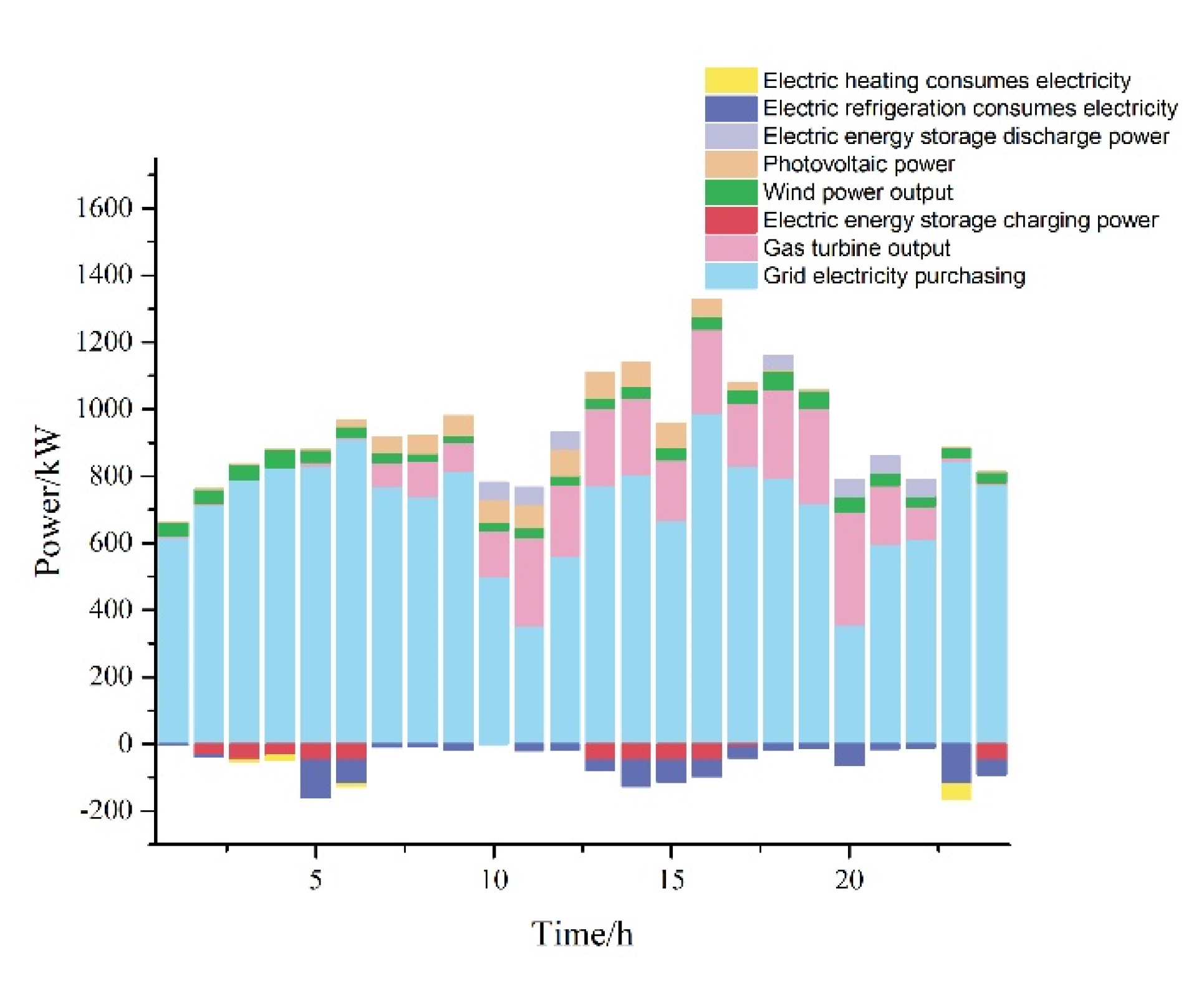
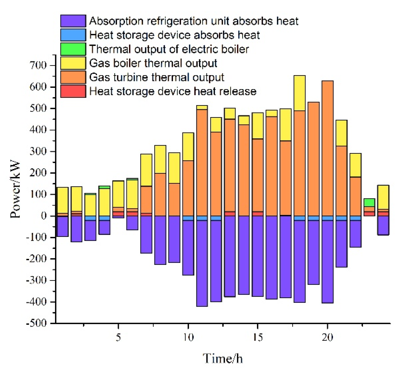
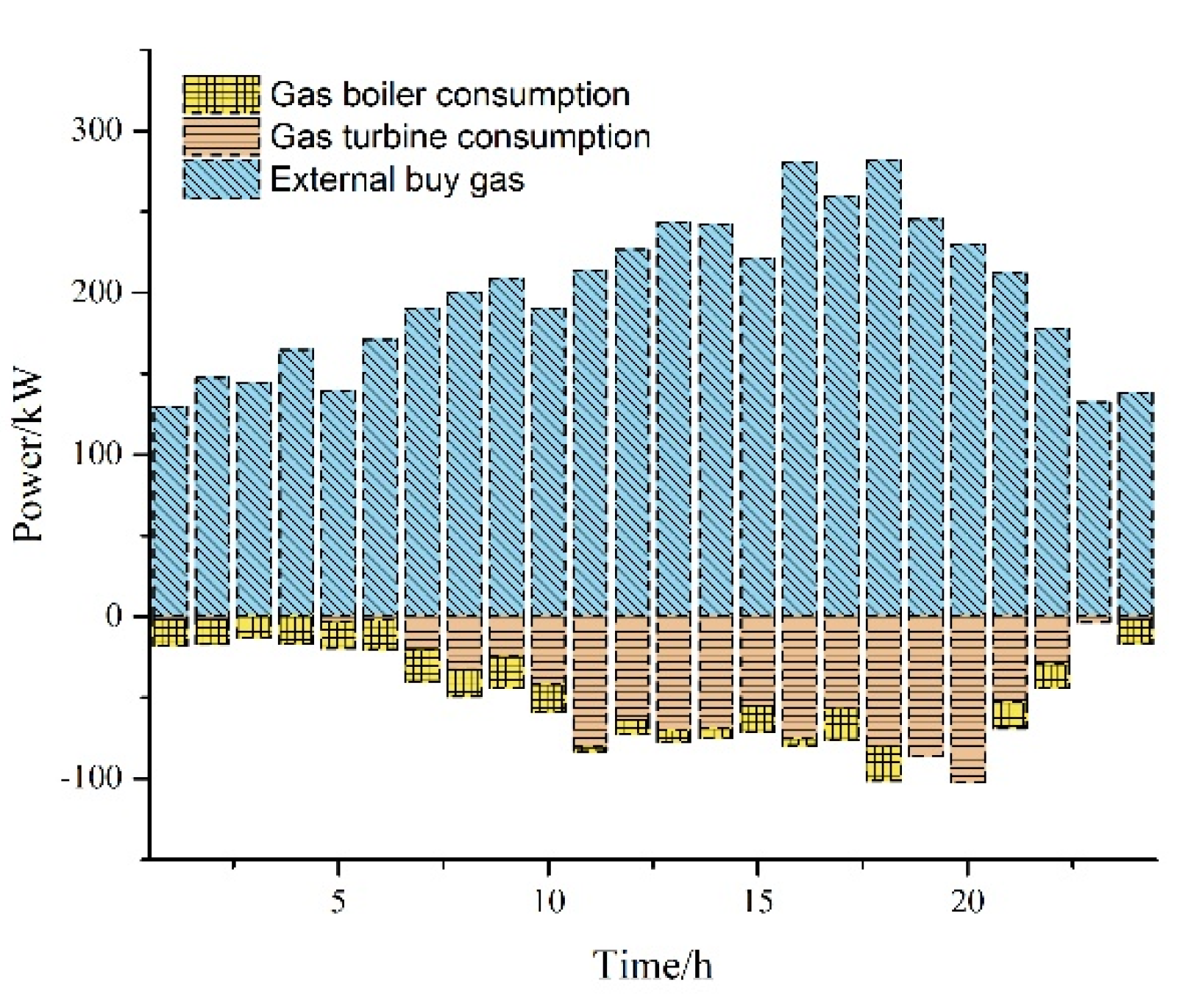
6.1. Optimization Results of Regional Integrated Energy System

The scheduling results of equipment in the RIES are shown in Figure 3, Figure 4, Figure 5, Figure 6, Figure 7 and Figure 8. During 1–6 and 23–24 h, the unit electricity price is lower, and the RIES mainly purchases power from the grid. At this time, the gas turbine runs at a lower power, and the electric boiler and electric refrigerator provide a small amount of heat energy and cold energy, respectively. At 7–12 h the electricity price rises, while the simultaneous electric load and cooling load gradually rise. At this time, the gas turbine power increases, while due to the increase in electricity price, the RIES purchases a lower proportion of electricity from the grid and flexibly relies on the discharge of electric energy storage equipment to balance the power load demand of the system. As a cogeneration unit, the heat energy provided by gas turbine rises with the increase in electric power output. At this time, the cooling load of the system is mainly generated by the absorption chiller absorbing heat energy, and a small amount of cooling load is provided by electric refrigeration equipment. From 12 to 17 h, the price of electricity decreases when it reaches a high peak value, the cooling load and heat load rise further and the electric load reaches the peak value at 16 h. Therefore, the proportion of purchased electricity and purchased electricity both rise, and the electric energy storage is charged to deal with the peak load in the late 18–22 h period. During 18–22 h, the price of electricity rises, while the heat and cold loads peak. At this time, the output of the gas turbine increases, and the thermal output of the gas turbine increases. The heat load at 19 and 20 h is completely provided by the gas turbine. The cooling load is mainly provided by the absorption chiller, and part of the cooling load is provided by the electric chiller. From 23 to 24 h, the electricity price falls to the lowest value, and the cold and heat loads decrease. Most of the electric loads are provided by the external purchasing power of the grid, and the proportion of electric refrigeration and heating increases.

In order to analyze the economy of the proposed method, the results of the two-stage robust optimal scheduling method were compared with those of the traditional deterministic scheduling method. Given that intra-day output deviation of wind and photovoltaic power is negative 15% and load deviation is positive 10%, in this scenario, the deterministic scheduling was compared with the two-stage scheduling conclusion proposed in this study, and day-ahead scheduling cost and intra-day scheduling energy purchase deviation cost were calculated as shown in

Table 1. Operational cost of RIES for different scheduling schemes.

Cost	Deterministic Optimization	Two-Stage Robust Optimization
Day-ahead dispatching cost	22,844.74	23,622.95
Cost of purchasing deviation	3883.77	1176.57
Total cost of electricity purchase	26,728.51	24,799.52

.

The purpose of the two-stage robust optimization constructed in this study is to minimize the total operating cost of the system in extreme scenarios. In this scenario, the day-ahead scheduling plan needs to satisfy the system constraints when the system uncertainty fluctuates the most so that the two-stage robust optimization day-ahead scheduling strategy is conservative. It can be seen from Table 1 that the day-ahead scheduling cost of two-stage robust optimization is higher than that of deterministic optimization method. In the diurnal scheduling stage, the difference between diurnal scheduling and real-time energy supply needs to be compensated by adjusting unit output. For the two-stage robust optimization, the conservative day-ahead scheduling makes it more flexible and the intra-day adjustment cost is relatively low. Therefore, the total operating cost of the operation strategy system proposed by the two-stage robust optimization is lower than that of the deterministic optimization. Therefore, compared with the deterministic optimization, the scheduling strategy based on the two-stage robust optimization has stronger robustness and has stronger ability to resist the fluctuating risks of wind and photovoltaic power and multi-energy loads.

6.2. Scenario Analysis

In order to verify the capability of two-stage robust optimization in dealing with wind, light and load uncertainties, four scenarios were designed for comparative analysis.

Scenario 1 is the basic case without considering the uncertainties of wind, light and load, and the robustness coefficient is ${\Gamma }^G={\Gamma }^L=0$;

Scenario 2 only considers the uncertainty of the power generation side, and the robustness coefficient is set as ${\Gamma }^G=16$, ${\Gamma }^L=0$;

In scenario 3, only load-side uncertainty is considered, and the robustness coefficient is set as ${\Gamma }^G=0$, ${\Gamma }^L=10$;

In scenario 4, both generator-side and load-side uncertainties are considered, and the robustness coefficient is set as ${\Gamma }^G=16$, ${\Gamma }^L=10$.

Day-ahead scheduling results, intra-day scheduling results and deviation coefficients in the four scenarios are shown in

Table 2. Comparison of day-ahead scheduling cost in different scenarios.

Cost	Scenario 1	Scenario 2	Scenario 3	Scenario 4
Power purchase cost	8174.69	8172.63	9108.11	9079.98
Purchase cost of gas	14,670.04	14,630.47	14,585.10	14,542.97
The total cost	22,844.74	22,803.10	23,693.21	23,622.95

.

When both source and load uncertainties are ignored, the day-ahead optimal operating cost is higher than that when load uncertainties are not considered. This because of the ignored load uncertainty and uncertain energy sources such as wind and light that depend on the forecast for scheduling, and there may be a positive deviation, increasing the system scheduling capacity. The system without scheduling at the present stage in response to increased possible load cost increases; therefore, scenario 2 has a scheduling stage cost comparable to scenario 1. Similarly, the pre-dispatch cost of scenario 4 decreases compared with scenario 3. The cost of day-ahead scheduling in scenario 3 is higher than that in scenario 1 because scenario 3 considers the load uncertainty in day-ahead scheduling, and the system needs to formulate strategies in day-ahead scheduling to deal with the deviation caused by load fluctuation. Therefore, the cost of day-ahead dispatching rises.

7. Conclusions

In this paper, a regional integrated energy system optimization method based on two-stage robust optimization is proposed, which takes into account the uncertainty of source-load on the east side of the RIES; establishes the combined optimization problem of energy conversion equipment, electricity storage and heat storage devices and gives the day-ahead scheduling and energy purchase scheme of the RIES. The validity of the method was verified by case analysis.

On the energy supply side, compared with previous studies that considered single energy, this study comprehensively considered the coupling characteristics of various energy sources, improved the absorption capacity of new energy and utilized the coupling characteristics of energy sources to suppress the fluctuation of the new energy grid-connected mode. On the load side, the uncertainty of the load side is added into the constraint, and the uncertainty of the load side is considered as well as the uncertainty of the energy supply side. In terms of model solving, it is difficult to obtain the probability distribution of random parameters in practical application, which limits the application of chance constrained programming, the probabilistic scenario method and the point estimation method. The global optimality of the solution efficiency and solution cannot be satisfied simultaneously because of the existence of non-convex constraints in chance-constrained programming. The computational efficiency and accuracy of the probabilistic scenario method are easily affected by the number of generated scenarios and the method of scene generation and reduction. In order to solve these problems, this paper proposes a column constraint algorithm to solve the model. The validity of the method was verified by case analysis.

The results show that:

(1)

The cost of day-purchase deviation obtained by the two-stage robust optimization method is lower than that obtained by the deterministic optimization method, while the traditional scheduling method does not consider the uncertain factors in advance, resulting in a large day-purchase deviation. The total cost of two-stage robust optimal scheduling is better than that of traditional deterministic scheduling methods.

(2)

Through the multi-energy coupling device and multi-energy coordination joint optimization, the proposed day-ahead scheduling strategy can effectively cope with the source-charge uncertainty in the day-ahead scheduling stage and enhance the robustness of the system.

(3)

By adjusting the uncertain budget value, RIES operators can flexibly adjust the scheduling conservatism of the RIES, which provides a reference for RIES operators to weigh the robustness and economy of the system.

References

1. Zhang, S.; Wang, K.; Xu, W.; Lyer-Raniga, U.; Athienitis, A.; Ge, H.; woo Cho, D.; Feng, W.; Okumiya, M.; Yoon, G.; et al. Policy recommendations for the zero energy building promotion towards carbon neutral in Asia-Pacific Region. Energy Policy 2021, 159, 112661. [Google Scholar] [CrossRef]
2. Song, S.; Li, T.; Liu, P.; Li, Z. The transition pathway of energy supply systems towards carbon neutrality based on a multi-regional energy infrastructure planning approach: A case study of China. Energy 2022, 1, 122037. [Google Scholar] [CrossRef]
3. Wu, H.; Xue, Y.; Hao, Y.; Ren, S. How does internet development affect energy-saving and emission reduction? Evidence from China. Energy Econ. 2021, 11, 105577. [Google Scholar] [CrossRef]
4. Miao, B.; Lin, J.; Li, H.; Liu, C.; Li, B.; Zhu, X.; Yang, J. Day-Ahead Energy Trading Strategy of Regional Integrated Energy System Considering Energy Cascade Utilization. IEEE Access 2020, 8, 138021–138035. [Google Scholar] [CrossRef]
5. Kumar, R.S.; Raghav, L.P.; Raju, D.K.; Singh, A.R. Intelligent demand side management for optimal energy scheduling of grid connected microgrids. Appl. Energy 2021, 285, 116435. [Google Scholar] [CrossRef]
6. Katiraei, F.; Iravani, R.; Hatziargyriou, N.; Dimeas, A. Microgrids management. IEEE Power Energy Mag. 2008, 6, 54–65. [Google Scholar] [CrossRef]
7. Liu, X.; Li, N.; Liu, F.; Mu, H.; Li, L.; Liu, X. Optimal Design on Fossil-to-Renewable Energy Transition of Regional Integrated Energy Systems under CO2 Emission Abatement Control: A Case Study in Dalian, China. Energies 2021, 14, 2879. [Google Scholar] [CrossRef]
8. Wang, Y.; Wang, J.; Liu, Z.; Liu, Y.; Tan, Z. Multi-objective synergy planning for regional integrated energy stations and networks considering energy interaction and equipment selection. Energy Convers. Manag. 2022, 1, 114986. [Google Scholar] [CrossRef]
9. Wang, Y.; Jiang, C.; Wen, F.; Xue, Y.; Chen, F.; Zhang, L.; Yuan, X. Energy Trading and Management Strategies in a Regional Integrated Energy System with Multiple Energy Carriers and Renewable-Energy Generation. J. Energy Eng. 2021, 147, 04020076. [Google Scholar] [CrossRef]
10. Li, X.; Wang, W.; Wang, H. A novel bi-level robust game model to optimize a regionally integrated energy system with large-scale centralized renewable-energy sources in Western China. Energy 2021, 8, 120513. [Google Scholar] [CrossRef]
11. Song, X.; Long, Y.; Tan, Z.; Zhang, X.; Li, L. The optimization of distributed photovoltaic comprehensive ef ciency based on the construction of regional integrated energy management system in China. Sustainability 2016, 11, 1201. [Google Scholar] [CrossRef] [Green Version]
12. Li, J.; Niu, D.; Wu, M.; Wang, Y.; Li, F.; Dong, H. Research on Battery Energy Storage as Backup Power in the Operation Optimization of a Regional Integrated Energy System. Energies 2018, 11, 2990. [Google Scholar] [CrossRef] [Green Version]
13. Lei, Y.; Wang, D.; Jia, H.; Chen, J.; Li, J.; Song, Y.; Li, J. Multi-objective stochastic expansion planning based on multi-dimensional correlation scenario generation method for regional integrated energy system integrated renewable energy. Appl. Energy 2020, 10, 115395. [Google Scholar] [CrossRef]
14. Wang, Y.; Huang, Y.; Wang, Y.; Zeng, M.; Yu, H.; Li, F.; Zhang, F. Optimal scheduling of the RIES considering time-based demand response programs with energy price. Energy 2018, 12, 733–793. [Google Scholar] [CrossRef]
15. Zhao, D.; Xia, X.; Tao, R. Optimal Configuration of Electric-Gas-Thermal Multi-Energy Storage System for Regional Integrated Energy System. Energies 2019, 7, 2586. [Google Scholar] [CrossRef] [Green Version]
16. Wang, J.; Li, P.; Fang, K.; Zhou, Y. Robust Optimization for Household Load Scheduling with Uncertain Parameters. Appl. Sci. 2018, 4, 575. [Google Scholar] [CrossRef] [Green Version]
17. Liu, C.; Wang, X.; Guo, J.; Huang, M.; Wu, X. Chance-constrained scheduling model of grid-connected microgrid based on probabilistic and robust optimization. IET Gener. Transm. Distrib. 2018, 12, 2499–2509. [Google Scholar] [CrossRef]
18. Zhong, J.; Wang, L.; Zhao, X.; Han, B. Research on optimisation of integrated energy system scheduling based on weak robust optimisation theory. IET Gener. Transm. Distrib. 2019, 13, 64–72. [Google Scholar]
19. Kim, H.J.; Kim, M.K.; Lee, J.W. A two-stage stochastic p-robust optimal energy trading management in microgrid operation considering uncertainty with hybrid demand response. Int. J. Electr. Power Energy Syst. 2021, 1, 106422. [Google Scholar] [CrossRef]
20. Wang, Y.; Tang, L.; Yang, Y.; Sun, W.; Zhao, H. A stochastic-robust coordinated optimization model for CCHP micro-grid considering multi-energy operation and power trading with electricity markets under uncertainties. Energy 2020, 198, 117273. [Google Scholar] [CrossRef]
21. Moretti, L.; Martelli, E.; Manzolini, G. An efficient robust optimization model for the unit commitment and dispatch of multi-energy systems and microgrids. Appl. Energy 2020, 3, 113859. [Google Scholar] [CrossRef]
22. Giraldo, J.S.; Castrillon, J.A.; L’opez, J.C.; Rider, M.J.; Castro, C.A. Microgrids energy management using robust convex programming. IEEE Trans. Smart Grid 2019, 10, 4520–4530. [Google Scholar] [CrossRef]
23. Zhao, H.; Wang, Y.; Zhao, M.; Tan, Q.; Guo, S. Day-ahead market modeling for strategic wind power producers under robust market clearing. Energies 2017, 10, 924. [Google Scholar] [CrossRef] [Green Version]
24. Zhu, J.; Huang, S.; Liu, Y.; Lei, H.; Sang, B. Optimal energy management for grid-connected microgrids via expected-scenario-oriented robust optimization. Energy 2021, 2, 119224. [Google Scholar] [CrossRef]
Figure 1. Schematic diagram of regional integrated energy system.
Energies 15 01596 g001
Figure 2. Flow chart of model solving.
Energies 15 01596 g002
Figure 3. Prediction interval of wind power and photovoltaic power output.
Energies 15 01596 g003
Figure 4. Prediction interval of load.
Energies 15 01596 g004
Figure 5. Prediction interval of wind power and photovoltaic power output.
Energies 15 01596 g005
Figure 6. Prediction interval of wind power and photovoltaic power output.
Energies 15 01596 g006
Figure 7. Prediction interval of wind power and photovoltaic power output.
Energies 15 01596 g007
Figure 8. Prediction interval of wind power and photovoltaic power output.
Energies 15 01596 g008