
Optimizing Multi Cross-Docking Systems with a Multi-Objective Green Location Routing Problem Considering Carbon Emission and Energy Consumption

 , , and
Abstract
:1. Introduction
- Developing a novel mathematical model to integrate CDS results in a comprehensive problem with a great application in industries;
- Making the problem closer to the real-world conditions by considering the effects of GHG emission in the transportation process and calculating energy consumption dependent on traffic time;
- Investigating the total cost minimization related to transportation, minimizing truck transportation sequences and carbon emissions through cross-docking simultaneously;
- Designing high-quality algorithms, including NSGA-II and MOPSO, efficiently to solve the large-sized problem.
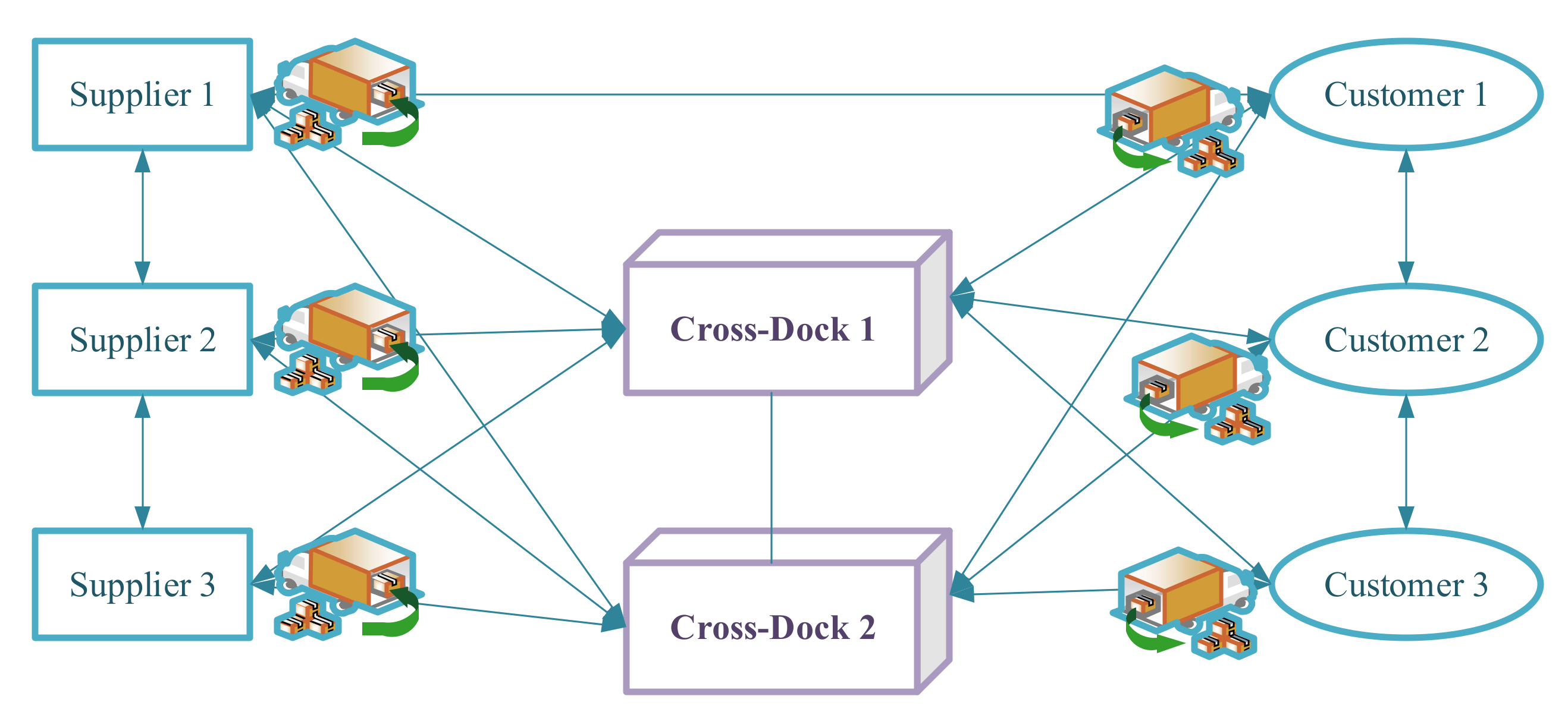
2. Problem Statements
- All incoming and outgoing trucks are available in zero time;
- Homogeneous vehicles with different capacities;
- Considering the period of customer service of norm type (having the earliest service start time and the latest service start time);
- Existence of several cross-docks so that suppliers choose one of the docks to send the goods considering the minimum cost;
- Ability to connect suppliers, docks, and customers with each other;
- The type and number of products supplied by suppliers, as well as the type and number of customer demand, are clear and constant;
- In the transport sequence, a truck can load products from more than one supplier and unload products from more than one customer;
- One or more suppliers may meet a customer’s requirements;
- The type and quantity of products transported by incoming trucks must be equal to the demands of customers.
2.1. Mathematical Model
2.2. Description of Objective Functions and Constraints
3. Solution Methodology
3.1. Genetic Algorithm
3.1.1. Chromosome Structure
3.1.2. The Structure of the Cross Method
3.1.3. Structure of the Mutation Method
3.2. Particle Swarm Optimization Algorithm—PSO
3.3. Validation of the Designed Model
Method of Generating Random Problems
4. Results
4.1. Comparison of NSGA-II and MOPSO Algorithms
4.1.1. Distance from the Ideal Point
4.1.2. Spacing
4.1.3. The Most Expansion
5. Conclusions and Suggestions
Author Contributions
Funding
Institutional Review Board Statement
Informed Consent Statement
Data Availability Statement
Conflicts of Interest
References
- Rijal, A.; Bijvank, M.; de Koster, R. Integrated scheduling and assignment of trucks at unit-load cross-dock terminals with mixed service mode dock doors. Eur. J. Oper. Res. 2019, 278, 752–771. [Google Scholar] [CrossRef]
- Serrano, C.; Delorme, X.; Dolgui, A. Scheduling of truck arrivals, truck departures and shop-floor operation in a cross-dock platform, based on trucks loading plans. Int. J. Prod. Econ. 2017, 194, 102–112. [Google Scholar] [CrossRef]
- Seyedi, I.; Hamedi, M.; Tavakkoli-Moghadaam, R. Developing a mathematical model for a multi-door cross-dock scheduling problem with human factors: A modified imperialist competitive algorithm. J. Ind. Eng. Manag. Stud. 2021, 8, 180–201. [Google Scholar]
- Motaghedi-Larijani, A.; Aminnayeri, M. Optimizing the admission time of outbound trucks entering a cross-dock with uniform arrival time by considering a queuing model. Eng. Optim. 2017, 49, 466–480. [Google Scholar] [CrossRef]
- Gelareh, S.; Glover, F.; Guemri, O.; Hanafi, S.; Nduwayo, P.; Todosijević, R. A comparative study of formulations for a cross-dock door assignment problem. Omega 2020, 91, 102015. [Google Scholar] [CrossRef]
- Xi, X.; Changchun, L.; Yuan, W.; Hay, L.L. Two-stage conflict robust optimization models for cross-dock truck scheduling problem under uncertainty. Transp. Res. Part E Logist. Transp. Rev. 2020, 144, 102123. [Google Scholar] [CrossRef]
- Sahebi, I.G.; Mosayebi, A.; Masoomi, B.; Marandi, F. Modeling the enablers for blockchain technology adoption in renewable energy supply chain. Technol. Soc. 2022, 101871. [Google Scholar] [CrossRef]
- Nassief, W. Cross-Dock Door Assignments: Models, Algorithms and Extensions. Ph.D. Thesis, Concordia University, Montréal, QC, Canada, 2017. Available online: https://spectrum.library.concordia.ca/id/eprint/982540/1/Nassief_PhD_S2017.pdf (accessed on 19 November 2021).
- Nasiri, M.M.; Rahbari, A.; Werner, F.; Karimi, R. Incorporating supplier selection and order allocation into the vehicle routing and multi-cross-dock scheduling problem. Int. J. Prod. Res. 2018, 56, 6527–6552. [Google Scholar] [CrossRef]
- Chargui, T.; Bekrar, A.; Reghioui, M.; Trentesaux, D. Simulation for Pi-hub cross-docking robustness. In Service Orientation in Holonic and Multi-Agent Manufacturing; Springer: Berlin, Germany, 2018; pp. 317–328. [Google Scholar]
- Tirkolaee, E.B.; Goli, A.; Faridnia, A.; Soltani, M.; Weber, G.-W. Multi-objective optimization for the reliable pollution-routing problem with cross-dock selection using Pareto-based algorithms. J. Clean. Prod. 2020, 276, 122927. [Google Scholar] [CrossRef]
- Wang, H.; Alidaee, B. The multi-floor cross-dock door assignment problem: Rising challenges for the new trend in logistics industry. Transp. Res. Part E Logist. Transp. Rev. 2019, 132, 30–47. [Google Scholar] [CrossRef]
- Dondo, R.; Cerdá, J. The heterogeneous vehicle routing and truck scheduling problem in a multi-door cross-dock system. Comput. Chem. Eng. 2015, 76, 42–62. [Google Scholar] [CrossRef]
- Zuluaga, J.P.S.; Thiell, M.; Perales, R.C. Reverse cross-docking. Omega 2017, 66, 48–57. [Google Scholar] [CrossRef]
- Mohtashami, A.; Tavana, M.; Santos-Arteaga, F.J.; Fallahian-Najafabadi, A. A novel multi-objective meta-heuristic model for solving cross-docking scheduling problems. Appl. Soft Comput. 2015, 31, 30–47. [Google Scholar] [CrossRef]
- Wisittipanich, W.; Hengmeechai, P. Truck scheduling in multi-door cross docking terminal by modified particle swarm optimization. Comput. Ind. Eng. 2017, 113, 793–802. [Google Scholar] [CrossRef]
- Mohtashami, A. A novel dynamic genetic algorithm-based method for vehicle scheduling in cross docking systems with frequent unloading operation. Comput. Ind. Eng. 2015, 90, 221–240. [Google Scholar] [CrossRef]
- Ponboon, S.; Qureshi, A.G.; Taniguchi, E. Evaluation of cost structure and impact of parameters in location-routing problem with time windows. Transp. Res. Procedia 2016, 12, 213–226. [Google Scholar] [CrossRef] [Green Version]
- Gomes, C.F.S.; Ribeiro, P.C.C.; de Matos Freire, K.A. Bibliometric research in Warehouse Management System from 2006 to 2016. In Proceedings of the World Multi-Conference on Systemics, Cybernetics and Informatics, Orlando, FL, USA, 8 July 2018; Volume 22, pp. 200–204. [Google Scholar]
- Birim, Ş. Vehicle routing problem with cross docking: A simulated annealing approach. Procedia Social Behav. Sci. 2016, 235, 149–158. [Google Scholar] [CrossRef]
- Yin, P.-Y.; Chuang, Y.-L. Adaptive memory artificial bee colony algorithm for green vehicle routing with cross-docking. Appl. Math. Model. 2016, 40, 9302–9315. [Google Scholar] [CrossRef]
- Mohtashami, A.; Fallahian-Najafabadi, A. Scheduling trucks transportation in supply chain regarding cross docking using meta-heuristic algorithms. Ind. Manag. Stud. 2014, 11, 55–84. [Google Scholar]
- Sung, C.S.; Song, S.H. Integrated service network design for a cross-docking supply chain network. J. Oper. Res. Soc. 2003, 54, 1283–1295. [Google Scholar] [CrossRef]
- Chen, P.; Guo, Y.; Lim, A.; Rodrigues, B. Multiple crossdocks with inventory and time windows. Comput. Oper. Res. 2006, 33, 43–63. [Google Scholar] [CrossRef] [Green Version]
- Sung, C.S.; Yang, W. An exact algorithm for a cross-docking supply chain network design problem. J. Oper. Res. Soc. 2008, 59, 119–136. [Google Scholar] [CrossRef]
- Wen, M.; Larsen, J.; Clausen, J.; Cordeau, J.-F.; Laporte, G. Vehicle routing with cross-docking. J. Oper. Res. Soc. 2009, 60, 1708–1718. [Google Scholar] [CrossRef] [Green Version]
- Musa, R.; Arnaout, J.-P.; Jung, H. Ant colony optimization algorithm to solve for the transportation problem of cross-docking network. Comput. Ind. Eng. 2010, 59, 85–92. [Google Scholar] [CrossRef]
- Dondo, R.; Méndez, C.A.; Cerdá, J. The multi-echelon vehicle routing problem with cross docking in supply chain management. Comput. Chem. Eng. 2011, 35, 3002–3024. [Google Scholar] [CrossRef]
- Santos, F.A.; Mateus, G.R.; Da Cunha, A.S. The pickup and delivery problem with cross-docking. Comput. Oper. Res. 2013, 40, 1085–1093. [Google Scholar] [CrossRef] [Green Version]
- Morais, V.W.C.; Mateus, G.R.; Noronha, T.F. Iterated local search heuristics for the vehicle routing problem with cross-docking. Expert Syst. Appl. 2014, 41, 7495–7506. [Google Scholar] [CrossRef]
- Vincent, F.Y.; Jewpanya, P.; Redi, A.A.N.P. Open vehicle routing problem with cross-docking. Comput. Ind. Eng. 2016, 94, 6–17. [Google Scholar]
- Wang, J.; Jagannathan, A.K.R.; Zuo, X.; Murray, C.C. Two-layer simulated annealing and tabu search heuristics for a vehicle routing problem with cross docks and split deliveries. Comput. Ind. Eng. 2017, 112, 84–98. [Google Scholar] [CrossRef]
- Rahbari, A.; Nasiri, M.M.; Werner, F.; Musavi, M.; Jolai, F. The vehicle routing and scheduling problem with cross-docking for perishable products under uncertainty: Two robust bi-objective models. Appl. Math. Model. 2019, 70, 605–625. [Google Scholar] [CrossRef]
- Baniamerian, A.; Bashiri, M.; Tavakkoli-Moghaddam, R. Modified variable neighborhood search and genetic algorithm for profitable heterogeneous vehicle routing problem with cross-docking. Appl. Soft Comput. 2019, 75, 441–460. [Google Scholar] [CrossRef]
- Zhou, B.; Zong, S. Adaptive memory red deer algorithm for cross-dock truck scheduling with products time window. Eng. Comput. 2021, 38, 3254–3289. [Google Scholar] [CrossRef]
- Liao, T.W. Integrated Outbound Vehicle Routing and Scheduling Problem at a Multi-Door Cross-Dock Terminal. IEEE Trans. Intell. Transp. Syst. 2020, 22, 5599–5612. [Google Scholar] [CrossRef]
- Safari, H.; Ajali, M.; Ghasemiyan Sahebi, I. Determining the strategic position of an educational institution in the organizational life cycle with fuzzy approach (Case Study: Social Sciences Faculty of Khalij Fars University). Mod. Res. Decis. Mak. 2016, 1, 117–138. [Google Scholar]
- Khalili-Damghani, K.; Tavana, M.; Santos-Arteaga, F.J.; Ghanbarzad-Dashti, M. A customized genetic algorithm for solving multi-period cross-dock truck scheduling problems. Measurement 2017, 108, 101–118. [Google Scholar] [CrossRef]
- Corsten, H.; Becker, F.; Salewski, H. Integrating truck and workforce scheduling in a cross-dock: Analysis of different workforce coordination policies. J. Bus. Econ. 2020, 90, 207–237. [Google Scholar] [CrossRef]
- Maknoon, Y.; Laporte, G. Vehicle routing with cross-dock selection. Comput. Oper. Res. 2017, 77, 254–266. [Google Scholar] [CrossRef]
- Eberhart, R.; Kennedy, J. A new optimizer using particle swarm theory. In Proceedings of the MHS’95. Proceedings of the Sixth International Symposium on Micro Machine and Human Science, Nagoya, Japan, 4–6 October 1995; pp. 39–43. [Google Scholar]
- Sahebi, I.; Masoomi, B.; Ghorbani, S.; Uslu, T. Scenario-based designing of closed-loop supply chain with uncertainty in returned products. Decis. Sci. Lett. 2019, 8, 505–518. [Google Scholar] [CrossRef]
- Kusolpuchong, S.; Chusap, K.; Alhawari, O.; Suer, G. A Genetic Algorithm Approach for Multi Objective Cross Dock Scheduling in Supply Chains. Procedia Manuf. 2019, 39, 1139–1148. [Google Scholar] [CrossRef]
- Arab, A.; Sahebi, I.G.; Modarresi, M.; Ajalli, M. A Grey DEMATEL approach for ranking the KSFs of environmental management system implementation (ISO 14001). Calitatea 2017, 18, 115. [Google Scholar]
- Arab, A.; Sahebi, I.G.; Alavi, S.A. Assessing the key success factors of knowledge management adoption in supply chain. Int. J. Acad. Res. Bus. Soc. Sci. 2017, 7, 2222–6990. [Google Scholar] [CrossRef] [Green Version]
- Sayed, S.I.; Contreras, I.; Diaz, J.A.; Luna, D.E. Integrated cross-dock door assignment and truck scheduling with handling times. Top 2020, 28, 705–727. [Google Scholar] [CrossRef]
- Heidari, F.; Zegordi, S.H.; Tavakkoli-Moghaddam, R. Modeling truck scheduling problem at a cross-dock facility through a bi-objective bi-level optimization approach. J. Intell. Manuf. 2018, 29, 1155–1170. [Google Scholar] [CrossRef]


| References | Multiple Cross-Docks | Type of Vehicle | Time Windows | Capacity in Crossdocks | Multiple Objectives | Solution Method | ||||
|---|---|---|---|---|---|---|---|---|---|---|
| Homogeneous | Heterogeneous | Limited | Unlimited | Exact | Heuristic | Metaheuristic | ||||
| [23] | * | * | * | * | ||||||
| [24] | * | * | * | * | * | |||||
| [25] | * | * | * | * | ||||||
| [26] | * | * | * | * | ||||||
| [27] | * | * | * | * | * | |||||
| [28] | * | * | * | * | * | |||||
| [29] | * | * | * | |||||||
| [30] | * | * | * | * | ||||||
| [31] | * | * | * | |||||||
| [32] | * | * | * | * | * | |||||
| [9] | * | * | * | * | * | * | ||||
| [33] | * | * | * | * | * | * | ||||
| [34] | * | * | * | * | ||||||
| [11] | * | * | * | * | * | * | ||||
| [35] | * | * | * | * | * | |||||
| Current research | * | * | * | * | * | * | * | |||
| Sets | |
|---|---|
| S | Set of suppliers (1,…,S) |
| C | Set of customers (1,…,C) |
| Set of incoming trucks (Receiving) (1,…,K) | |
| Set of outgoing trucks (Sending) (1,…,K’) | |
| G | Set of products type (order) (1,…,G) |
| Cd | Set of Cross-docks (1,…,Z) |
| Parameters | |
| Transportation time | |
| Time of entry or exit of incoming truck (i) from supplier (s), while loading the order of type (G) and moving towards the customer (c) | |
| When the incoming truck (j) enters to the customer (c) from the cross-dock (cd) while loading the order of type (G) | |
| Transportation time of incoming truck (i) from supplier (s) to customer (c) while loading the order of type (G) | |
| Transport time of outgoing truck (j) from cross-dock (cd) to customer (c), while loading the order of type (G) | |
| Offloading time of each product type (G) from input truck (i) to customer (c) | |
| Offloading time of each product type (G) from output truck (j) to customer (c) | |
| Customer order (c) of type (G) goods | |
| Production rate of product with type (G) | |
| Weight of product with type (G) | |
| Demand of customer (i) | |
| Time window interval of customer (i) | |
| Early arrival time of incoming or outgoing truck in the time window | |
| Incoming or outgoing truck late arrival time | |
| Penalty for delay or early arrival of a vehicle exiting the cross-dock (i) for the customer (c) | |
| Penalty for delay or early arrival of the incoming vehicle from the supplier (i) to the customer (i) | |
| Vehicle waiting time at the location of customer (c) | |
| Cost of reopening the cross-dock (i) | |
| Capacity of incoming truck (i) | |
| Capacity of output truck (i) | |
| Distance between supplier (s) and cross-dock (cd) | |
| Distance between supplier (s) and customer (c) | |
| Distance between cross-dock (cd) and customer (c) | |
| The fuel conversion rate of the unloaded incoming truck to carbon dioxide | |
| The difference between the conversion rate of the fuel of an incoming truck with a load of one unit of product or more with the same truck without a load of carbon dioxide | |
| The difference between the conversion rate of the fuel of an outgoing truck with a load of one unit of product or more with the same truck without a load of carbon dioxide | |
| Conversion rate of unloaded truck fuel into CO2 | |
| Incoming truck fuel consumption rate for travel between supplier (s) and customer (c) without load | |
| The fuel consumption rate of incoming trucks for travel between supplier (s) and cross-dock (cd) without load | |
| Incoming truck fuel consumption rate for travel between the source supplier (s) and the destination supplier without load | |
| Incoming truck fuel consumption rate for travel between the cross-dock (cd) of origin and the cross-dock of destination without cargo | |
| Outgoing truck fuel consumption rate for travel between origin and destination customer (c) without load | |
| Outgoing truck fuel consumption rate for travel between cross-dock (cd) and customer (c) without load | |
| The difference in the fuel consumption rate of an incoming truck traveling with one product or more with the same unladen truck | |
| The difference in the fuel consumption rate of an outgoing truck traveling with one product or more with the same unladen truck | |
| The number of product types (G) the truck carries between supplier (s) and cross-dock (cd) | |
| The number of product types (G) the truck carries between supplier (s) and the customer (c) | |
| The number of product types (G) the truck carries between cross-dock (cd) and customer (c) | |
| The number of product types (G) the truck carries between source supplier and destination supplier | |
| The number of product types (G) the truck carries between source customer and destination customer | |
| The number of product types (G) the truck carries between source cross-dock and destination cross-dock | |
| Big number | |
| Variables | |
| The number of product types (G) that are loaded from the supplier (s) into the input truck (i) | |
| The number of product types (G) that are loaded from the cross-dock (cd) into the output truck (j) | |
| The number of product types (G) that are unloaded from the incoming truck (i) at the customer’s location | |
| Source | S1 | S2 | CD1 | CD2 | S1S2 | S1CD1 | S1CD2 | S2CD1 | S2CD2 | CD1CD2 | S1S2CD1 | S1S2CD2 | S1S2CD1CD2 |
|---|---|---|---|---|---|---|---|---|---|---|---|---|---|
| CD1 | 1 | 1 | 0 | 1 | 1 | 0 | 1 | 0 | 1 | 0 | 1 | 1 | 1 |
| S1 | 0 | 0 | 0 | 0 | 0 | 0 | 0 | 1 | 1 | 1 | 0 | 0 | 0 |
| CD2 | 0 | 0 | 1 | 0 | 1 | 1 | 0 | 1 | 0 | 0 | 1 | 1 | 1 |
| S2 | 0 | 0 | 0 | 0 | 0 | 1 | 1 | 0 | 0 | 1 | 1 | 1 | 1 |
| Destination | C1 | C2 | CD1 | CD2 | C1C2 | C1CD1 | C1CD2 | C2CD1 | C2CD2 | C1C2CD1 | C1C2CD2 | C1C2CD1CD2 |
|---|---|---|---|---|---|---|---|---|---|---|---|---|
| CD1 | 1 | 1 | 0 | 0 | 1 | 1 | 1 | 0 | 1 | 1 | 1 | 1 |
| C1 | 0 | 0 | 0 | 0 | 0 | 0 | 0 | 1 | 1 | 0 | 0 | 0 |
| CD2 | 0 | 0 | 1 | 0 | 1 | 1 | 0 | 1 | 0 | 1 | 1 | 1 |
| C2 | 0 | 0 | 0 | 1 | 0 | 0 | 1 | 0 | 0 | 0 | 0 | 0 |
| Ordering Mode | A | B | C | D | AB | AC | AD | BC | BD | CD | ABC | ABD | ACD | BCD | ABCD |
|---|---|---|---|---|---|---|---|---|---|---|---|---|---|---|---|
| A | 1 | 0 | 0 | 0 | 1 | 1 | 1 | 0 | 0 | 0 | 1 | 1 | 1 | 0 | 1 |
| B | 0 | 1 | 0 | 0 | 1 | 0 | 0 | 1 | 1 | 0 | 1 | 1 | 0 | 1 | 1 |
| C | 0 | 0 | 1 | 0 | 0 | 1 | 0 | 1 | 0 | 1 | 1 | 0 | 1 | 1 | 1 |
| D | 0 | 0 | 0 | 1 | 0 | 0 | 1 | 0 | 1 | 1 | 0 | 1 | 1 | 1 | 1 |
| First Parent | ||||||||||||
|---|---|---|---|---|---|---|---|---|---|---|---|---|
| 1 | 1 | 0 | 1 | 1 | 0 | 1 | 0 | 1 | 0 | 1 | 1 | 1 |
| 0 | 0 | 0 | 0 | 0 | 0 | 0 | 1 | 1 | 1 | 0 | 0 | 0 |
| 0 | 0 | 1 | 0 | 1 | 1 | 0 | 1 | 0 | 0 | 1 | 1 | 1 |
| 0 | 0 | 0 | 0 | 0 | 1 | 1 | 0 | 0 | 1 | 1 | 1 | 1 |
| Second Parent | ||||||||||||
| 0 | 0 | 0 | 1 | 0 | 0 | 0 | 1 | 0 | 0 | 1 | 1 | 1 |
| 0 | 1 | 0 | 0 | 0 | 0 | 0 | 0 | 1 | 1 | 0 | 0 | 0 |
| 1 | 0 | 0 | 0 | 1 | 1 | 0 | 1 | 1 | 0 | 1 | 0 | 1 |
| 0 | 0 | 1 | 0 | 1 | 1 | 1 | 0 | 0 | 1 | 1 | 1 | 1 |
| The First Child | ||||||||||||
|---|---|---|---|---|---|---|---|---|---|---|---|---|
| 0 | 0 | 0 | 1 | 0 | 0 | 0 | 1 | 1 | 0 | 1 | 1 | 1 |
| 0 | 1 | 0 | 0 | 0 | 0 | 1 | 1 | 1 | 1 | 0 | 0 | 0 |
| 1 | 0 | 0 | 0 | 1 | 1 | 1 | 0 | 0 | 0 | 1 | 1 | 1 |
| 0 | 0 | 1 | 0 | 0 | 1 | 1 | 0 | 0 | 1 | 1 | 1 | 1 |
| The Second Child | ||||||||||||
| 1 | 1 | 0 | 1 | 1 | 0 | 0 | 1 | 0 | 0 | 1 | 1 | 1 |
| 0 | 0 | 0 | 0 | 0 | 0 | 0 | 0 | 1 | 1 | 0 | 0 | 0 |
| 0 | 0 | 1 | 0 | 1 | 1 | 0 | 1 | 1 | 0 | 1 | 0 | 1 |
| 0 | 0 | 0 | 0 | 1 | 1 | 1 | 0 | 0 | 1 | 1 | 1 | 1 |
| The First Child | ||||||||||||
|---|---|---|---|---|---|---|---|---|---|---|---|---|
| 0 | 0 | 0 | 1 | 0 | 0 | 0 | 1 | 0 | 0 | 1 | 1 | 1 |
| 0 | 1 | 0 | 0 | 0 | 0 | 0 | 0 | 1 | 1 | 0 | 0 | 0 |
| 0 | 0 | 1 | 0 | 1 | 1 | 0 | 1 | 0 | 0 | 1 | 1 | 1 |
| 0 | 0 | 0 | 0 | 0 | 1 | 1 | 0 | 0 | 1 | 1 | 1 | 1 |
| The Second Child | ||||||||||||
| 1 | 1 | 0 | 1 | 1 | 0 | 1 | 0 | 1 | 0 | 1 | 1 | 1 |
| 0 | 0 | 0 | 0 | 0 | 0 | 0 | 1 | 1 | 1 | 0 | 0 | 0 |
| 1 | 0 | 0 | 0 | 1 | 1 | 0 | 1 | 1 | 0 | 1 | 0 | 1 |
| 0 | 0 | 1 | 0 | 1 | 1 | 1 | 0 | 0 | 1 | 1 | 1 | 1 |
| The First Child | ||||||||||||
|---|---|---|---|---|---|---|---|---|---|---|---|---|
| 1 | 1 | 0 | 1 | 1 | 0 | 1 | 0 | 1 | 0 | 1 | 1 | 1 |
| 0 | 0 | 0 | 0 | 0 | 0 | 0 | 1 | 1 | 1 | 0 | 0 | 0 |
| 0 | 0 | 1 | 0 | 1 | 1 | 0 | 1 | 0 | 0 | 1 | 1 | 1 |
| 0 | 0 | 0 | 0 | 0 | 1 | 1 | 0 | 0 | 1 | 1 | 1 | 1 |
| The Second Child | ||||||||||||
| 0 | 0 | 0 | 1 | 1 | 0 | 1 | 0 | 1 | 0 | 1 | 1 | 1 |
| 0 | 0 | 0 | 0 | 0 | 0 | 0 | 1 | 1 | 1 | 0 | 0 | 0 |
| 1 | 0 | 0 | 0 | 1 | 1 | 0 | 1 | 0 | 0 | 1 | 1 | 1 |
| 0 | 0 | 1 | 0 | 0 | 1 | 1 | 0 | 0 | 1 | 1 | 1 | 1 |
| 1 | 1 | 0 | 1 | 1 | 0 | 1 | 0 | 1 | 0 | 1 | 1 | 1 |
| 0 | 0 | 0 | 0 | 0 | 0 | 0 | 1 | 1 | 1 | 0 | 0 | 0 |
| 0 | 0 | 1 | 0 | 0 | 1 | 0 | 1 | 0 | 0 | 1 | 1 | 1 |
| 0 | 0 | 0 | 0 | 0 | 1 | 1 | 0 | 0 | 1 | 1 | 1 | 1 |
| 1 | 1 | 0 | 1 | 1 | 0 | 1 | 0 | 1 | 0 | 1 | 1 | 1 |
| 1 | 1 | 1 | 1 | 1 | 1 | 1 | 0 | 0 | 0 | 1 | 1 | 1 |
| 0 | 0 | 1 | 0 | 1 | 1 | 0 | 1 | 0 | 0 | 1 | 1 | 1 |
| 0 | 0 | 0 | 0 | 0 | 1 | 1 | 0 | 0 | 1 | 1 | 1 | 1 |
| 1 | 1 | 0 | 1 | 1 | 0 | 0 | 0 | 1 | 0 | 1 | 1 | 1 |
| 0 | 0 | 0 | 0 | 0 | 0 | 1 | 1 | 1 | 1 | 0 | 0 | 0 |
| 0 | 0 | 1 | 0 | 1 | 1 | 1 | 1 | 0 | 0 | 1 | 1 | 1 |
| 0 | 0 | 0 | 0 | 0 | 1 | 0 | 0 | 0 | 1 | 1 | 1 | 1 |
| For each particle Initialize particle End For Do For each particle Calculate fitness value of the particle fp /*updating particle’s best fitness value so far)*/ If fp is better than pBest set current value as the new pBest End For /*updating population’s best fitness value so far)*/ Set gBest to the best fitness value of all particles For each particle Calculate particle velocity according to equation Update particle position according to equation End For While maximum iterations OR minimum error criteria is not attained |
| Parameters | Problem 1 | Problem 2 | Problem 3 | ||||||||||||||||||
|---|---|---|---|---|---|---|---|---|---|---|---|---|---|---|---|---|---|---|---|---|---|
| 1 | 2 | 3 | 4 | 5 | 6 | 7 | 1 | 2 | 3 | 4 | 5 | 6 | 7 | 1 | 2 | 3 | 4 | 5 | 6 | 7 | |
| Number of incoming trucks | 2 | 4 | 4 | 3 | 4 | 3 | 3 | 3 | 4 | 2 | 4 | 4 | 3 | 3 | 12 | 11 | 13 | 14 | 11 | 12 | 11 |
| Number of outgoing trucks | 2 | 4 | 3 | 4 | 4 | 3 | 2 | 2 | 3 | 3 | 2 | 3 | 2 | 2 | 11 | 12 | 11 | 12 | 11 | 10 | 12 |
| Number of suppliers | 4 | 3 | 4 | 4 | 5 | 3 | 2 | 10 | 9 | 9 | 8 | 7 | 8 | 11 | 18 | 17 | 17 | 19 | 18 | 16 | 20 |
| Number of cross- dock | 4 | 3 | 3 | 7 | 4 | 3 | 3 | 8 | 9 | 9 | 7 | 8 | 6 | 6 | 12 | 10 | 11 | 12 | 10 | 10 | 14 |
| Product types | 10 | 6 | 8 | 10 | 9 | 10 | 11 | 12 | 12 | 14 | 12 | 11 | 13 | 15 | 20 | 16 | 18 | 20 | 20 | 20 | 25 |
| Number of customer | 5 | 3 | 4 | 8 | 4 | 3 | 3 | 11 | 12 | 10 | 9 | 10 | 11 | 15 | 22 | 20 | 23 | 21 | 20 | 18 | 20 |
| Customer demand | U(0,30) | U(0,30) | U(0,30) |
| Product supply rate | U(0,30) | U(0,30) | U(0,30) |
| Product weight | U(0,10) | U(0,10) | U(0,10) |
| Incoming truck capacity | U(0,10) × 1000 | U(0,10) × 1000 | U(0,10) × 1000 |
| Outgoing trucks capacity | U(0,10) × 1000 | U(0,10) × 1000 | U(0,10) × 1000 |
| Origin between destination distance | U(1,100) | U(1,100) | U(1,100) |
| Number of product type G | U(1,10) | U(1,10) | U(1,10) |
| Fuel consumption rate | U(1,20) | U(1,20) | U(1,20) |
| Algorithm | Parameters | Parameter Domin | Amounts |
|---|---|---|---|
| NSGA-II | Iteration | 100–300 | 300 |
| Population size | 50–100 | 100 | |
| Intersection rate | 0.6–0.8 | 0.8 | |
| Mutation rate | 0.1–0.2 | 0.2 | |
| MOPSO | Iteration | 100–300 | 300 |
| Population size | 50–100 | 100 | |
| Cognitive constants, C1 | 1–3 | 3 | |
| Social constant, C2 | 1–2 | 2 |
| Origin | Destination | Product Type | Number of Products | Shipping Sequence |
|---|---|---|---|---|
| Supplier 1 | Cross-dock 1 | E | 7 | 1 |
| Supplier 2 | Cross-dock 1 | F | 15 | |
| Supplier 3 | Cross-dock 3 | G | 6 | 2 |
| Supplier 3 | Customer 1 | D | 14 | |
| Supplier 3 | Customer 2 | D | 14 | |
| Supplier 2 | Customer 3 | D | 13 | |
| Supplier 1 | Customer 3 | E | 17 | |
| Supplier 2 | Customer 1 | F | 8 | 3 |
| Supplier 2 | Customer 2 | F | 16 | |
| Supplier 2 | Customer 3 | F | 18 | |
| Supplier 2 | Customer 2 | G | 7 | |
| Supplier 3 | Supplier 1 | E | 7 | |
| Supplier 2 | Supplier 1 | F | 15 | |
| Supplier 3 | Supplier 1 | F | 16 | 4 |
| Cross-dock 3 | Cross-dock 1 | D | 14 | 5 |
| Cross-dock 2 | Cross-dock 1 | F | 16 | |
| Customer 3 | Customer 1 | D | 14 | |
| Customer 3 | Customer 2 | E | 8 | |
| Customer 3 | Customer 2 | F | 18 | |
| Customer 3 | Customer 2 | G | 13 | 6 |
| Cross-dock 1 | Customer 1 | B | 9 | |
| Cross-dock 1 | Customer 3 | D | 14 | |
| Cross-dock 1 | Customer 1 | G | 10 | |
| Cross-dock 1 | Customer 2 | G | 7 | |
| Cross-dock 2 | Customer 3 | C | 11 | 7 |
| Cross-dock 3 | Customer 1 | E | 17 |
| Origin | Destination | Product Type | Number of Products | Shipping Sequence |
|---|---|---|---|---|
| Supplier 2 | Cross-dock 2 | D | 8 | |
| Supplier 2 | Cross-dock 2 | E | 8 | |
| Supplier 2 | Cross-dock 2 | H | 11 | 1 |
| Supplier 2 | Customer 1 | D | 14 | |
| Supplier 2 | Customer 2 | D | 13 | |
| Supplier 2 | Customer 1 | E | 17 | |
| Supplier 2 | Customer 2 | E | 4 | 2 |
| Supplier 2 | Customer 3 | E | 8 | |
| Supplier 1 | Customer 3 | D | 14 | |
| Supplier 2 | Supplier 1 | D | 8 | |
| Supplier 2 | Supplier 1 | H | 11 | 3 |
| Cross-dock 2 | Cross-dock 1 | D | 12 | 4 |
| Customer 3 | Customer 2 | E | 8 | |
| Customer 1 | Customer 2 | H | 4 | 5 |
| Cross-dock 2 | Customer 3 | C | 17 | |
| Cross-dock 2 | Customer 1 | E | 17 | |
| Cross-dock 2 | Customer 2 | E | 4 | |
| Cross-dock 2 | Customer 3 | G | 7 | |
| Cross-dock 1 | Customer 3 | E | 17 | 6 |
| Cross-dock 3 | Customer 2 | E | 8 |
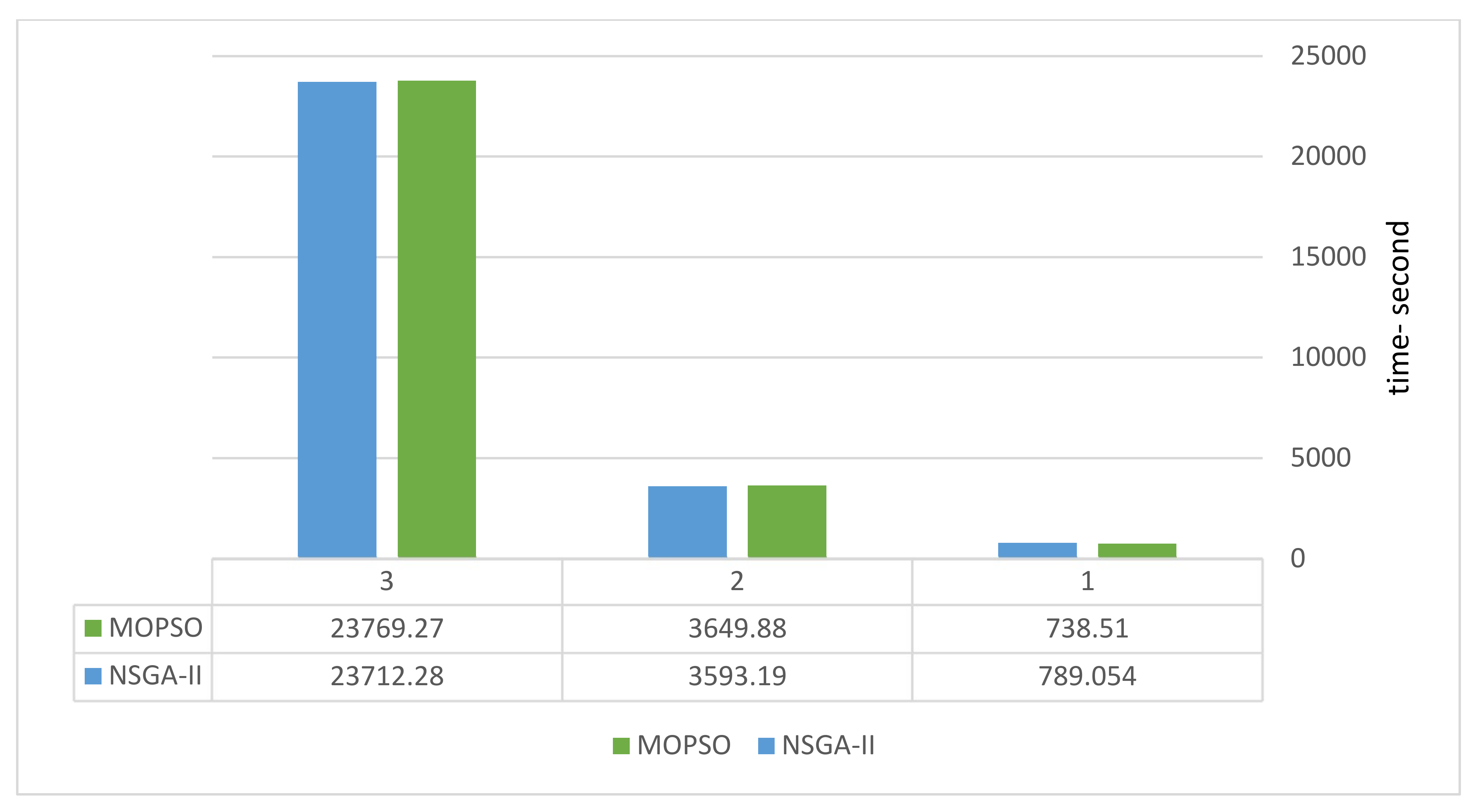
| Example | Size | NSGA-II | ||||
|---|---|---|---|---|---|---|
| NPS | Time (S) | MID | DM | Spacing | ||
| 1 | Small | 100 | 878.22 | 1.0918 | 50964 | 0.8515 |
| 2 | Small | 97 | 526.19 | 1.0601 | 3351 | 0.9425 |
| 3 | Small | 100 | 898.23 | 1.0361 | 5745.4 | 0.9863 |
| 4 | Small | 100 | 1204.84 | 1.1609 | 5082.3 | 0.8294 |
| 5 | Small | 100 | 911.26 | 1.0537 | 5281.4 | 0.9158 |
| 6 | Small | 99 | 392.67 | 1.0077 | 3667.4 | 0.9317 |
| 7 | Small | 99 | 711.97 | 1.1094 | 4616 | 1.0001 |
| Mean | 99.28 | 798.054 | 1.0742 | 4691.4 | 0.9226 | |
| 1 | Middle | 100 | 2011.51 | 1.0466 | 9406.5 | 0.8803 |
| 2 | Middle | 100 | 2213.24 | 1.0494 | 9415 | 0.9962 |
| 3 | Middle | 100 | 3415.81 | 1.0453 | 11,761 | 1.0038 |
| 4 | Middle | 100 | 4313.86 | 1.043 | 11,291 | 1.0075 |
| 5 | Middle | 100 | 4201.49 | 1.0371 | 12,580 | 1.0718 |
| 6 | Middle | 100 | 3919.35 | 1.0394 | 13,449 | 0.9942 |
| 7 | Middle | 99 | 5077.08 | 1.0556 | 12,997 | 0.963 |
| Mean | 99.85 | 3593.19 | 1.045 | 11,557.07 | 0.9881 | |
| 1 | Large | 100 | 19,202.23 | 1.0627 | 19,654 | 1.1429 |
| 2 | Large | 99 | 21,020.54 | 1.0748 | 21,012 | 1.1436 |
| 3 | Large | 100 | 210,695.14 | 1.0452 | 20,654.12 | 1.1259 |
| 4 | Large | 100 | 230,458.87 | 1.0872 | 23,012.45 | 1.1248 |
| 5 | Large | 100 | 26,748.65 | 1.0925 | 24,896.87 | 1.0258 |
| 6 | Large | 99 | 25,874.96 | 1.0745 | 23,968.97 | 1.0387 |
| 7 | Large | 100 | 27,987.56 | 1.0998 | 25,984.23 | 1.0587 |
| Mean | 99.714 | 22,715.28 | 1.0766 | 22,624.79 | 1.0941 | |
| Example | Size | MOPSO | ||||
|---|---|---|---|---|---|---|
| NPS | Time (S) | MID | DM | Spacing | ||
| 1 | Small | 100 | 817.45 | 1.1166 | 2708.6 | 0.8495 |
| 2 | Small | 77 | 473.64 | 1.1234 | 1365.3 | 0.803 |
| 3 | Small | 99 | 831.9 | 1.0548 | 2972.3 | 0.9092 |
| 4 | Small | 94 | 1161.45 | 1.2043 | 2897.9 | 0.7604 |
| 5 | Small | 95 | 853.09 | 1.0943 | 3108.5 | 0.8189 |
| 6 | Small | 98 | 381.79 | 1.0829 | 2430 | 0.907 |
| 7 | Small | 95 | 650.25 | 1.1492 | 2324.6 | 0.7806 |
| Mean | 94 | 738.51 | 1.1179 | 2453.88 | 0.8326 | |
| 1 | Middle | 100 | 2044.69 | 1.0468 | 6090.3 | 0.9312 |
| 2 | Middle | 92 | 2320.03 | 1.0455 | 7155.5 | 1.0476 |
| 3 | Middle | 100 | 3451.65 | 1.0547 | 6141 | 0.8661 |
| 4 | Middle | 98 | 4364.47 | 1.049 | 7536.4 | 1.0063 |
| 5 | Middle | 98 | 4113.73 | 1.0404 | 7265.8 | 0.9996 |
| 6 | Middle | 100 | 3996.17 | 1.0364 | 8293.4 | 0.9286 |
| 7 | Middle | 96 | 5258.46 | 1.0625 | 6351.8 | 0.8655 |
| Mean | 97.714 | 3649.88 | 1.0479 | 6976.3 | 0.9493 | |
| 1 | Large | 100 | 19,795.71 | 1.0877 | 10395 | 0.8874 |
| 2 | Large | 100 | 22,101.36 | 1.0689 | 11,256 | 0.8658 |
| 3 | Large | 100 | 20,985.87 | 1.0589 | 10,365.85 | 0.8953 |
| 4 | Large | 100 | 21,895.3 | 1.0489 | 12,365.35 | 0.9587 |
| 5 | Large | 96 | 27,014.32 | 1.0845 | 12,985.36 | 0.8596 |
| 6 | Large | 100 | 26,579.89 | 1.0895 | 12,645.84 | 0.9741 |
| 7 | Large | 93 | 28,012.56 | 1.0114 | 13,586.96 | 0.8254 |
| Mean | 98.42 | 23,769.27 | 1.06 | 11,942.91 | 0.8951 | |
Publisher’s Note: MDPI stays neutral with regard to jurisdictional claims in published maps and institutional affiliations. |
© 2022 by the authors. Licensee MDPI, Basel, Switzerland. This article is an open access article distributed under the terms and conditions of the Creative Commons Attribution (CC BY) license (https://creativecommons.org/licenses/by/4.0/).
Share and Cite
Meidute-Kavaliauskiene, I.; Sütütemiz, N.; Yıldırım, F.; Ghorbani, S.; Činčikaitė, R. Optimizing Multi Cross-Docking Systems with a Multi-Objective Green Location Routing Problem Considering Carbon Emission and Energy Consumption. Energies 2022, 15, 1530. https://doi.org/10.3390/en15041530
Meidute-Kavaliauskiene I, Sütütemiz N, Yıldırım F, Ghorbani S, Činčikaitė R. Optimizing Multi Cross-Docking Systems with a Multi-Objective Green Location Routing Problem Considering Carbon Emission and Energy Consumption. Energies. 2022; 15(4):1530. https://doi.org/10.3390/en15041530
Chicago/Turabian StyleMeidute-Kavaliauskiene, Ieva, Nihal Sütütemiz, Figen Yıldırım, Shahryar Ghorbani, and Renata Činčikaitė. 2022. "Optimizing Multi Cross-Docking Systems with a Multi-Objective Green Location Routing Problem Considering Carbon Emission and Energy Consumption" Energies 15, no. 4: 1530. https://doi.org/10.3390/en15041530
APA StyleMeidute-Kavaliauskiene, I., Sütütemiz, N., Yıldırım, F., Ghorbani, S., & Činčikaitė, R. (2022). Optimizing Multi Cross-Docking Systems with a Multi-Objective Green Location Routing Problem Considering Carbon Emission and Energy Consumption. Energies, 15(4), 1530. https://doi.org/10.3390/en15041530