Developing and Field Testing a Green Light Optimal Speed Advisory System for Buses

Abstract

In this study, a Green Light Optimal Speed Advisory (GLOSA) system for buses (B-GLOSA) was developed. The proposed B-GLOSA system was implemented on diesel buses, and field tested to validate and quantify the potential real-world benefits. The developed system includes a simple and easy-to-calibrate fuel consumption model that computes instantaneous diesel bus fuel consumption rates. The bus fuel consumption model, a vehicle dynamics model, the traffic signal timings, and the relationship between vehicle speed and distance to the intersection are used to construct an optimization problem. A moving-horizon dynamic programming problem solved using the A-star algorithm is used to compute the energy-optimized vehicle trajectory through signalized intersections. The Virginia Smart Road test facility was used to conduct the field test on 30 participants. Each participant drove three scenarios, including a base case uninformed drive, an informed drive with signal timing information communicated to the driver, and an informed drive with the recommended speed computed by the B-GLOSA system. The field test investigated the performance of using the developed B-GLOSA system considering different impact factors, including road grades and red indication offsets, using a split-split-plot experimental design. The test results demonstrated that the proposed B-GLOSA system can produce smoother bus trajectories through signalized intersections, thus producing fuel consumption and travel time savings. Specifically, compared to the uninformed drive, the B-GLOSA system produces fuel and travel time savings of 22.1% and 6.1%, on average, respectively.

1. Introduction

Previous studies have shown that the fuel consumption rates are dramatically increased when vehicles approach signalized intersections, which is caused by vehicle acceleration and deceleration maneuvers [1,2]. Furthermore, knowledge of traffic signal phase and timing (SPaT) has been proven to benefit the energy use of vehicles by reducing stop-and-go maneuvers and idling time at signalized intersections [3]. With the development of information and communication technology, the advanced communication power in a connected vehicle (CV) environment ensures that a very high update rate of information can be provided to vehicles. For example, SPaT information, vehicle speed, and surrounding vehicle locations can be shared using vehicle-to-infrastructure (V2I) and vehicle-to-vehicle (V2V) communications. Such information can greatly help transportation scientists to develop and implement connected traffic systems to enhance traffic safety, efficiency, and energy usage. The fast-growing information and communication technologies are widely used in various ITS applications. During the past decade, many cutting-edge ITS technologies have been developed to enhance traffic control using V2I and V2V technologies, including eco-driving, eco-routing, and large-scale signal control. An eco-driving algorithm has been developed and implemented in traffic simulation software to generate fuel-optimum vehicle trajectories by using signal phasing and timing information [4]. The study in [5] quantifies the system-wide impacts of implementing a dynamic eco-routing system. The simulation results demonstrate that eco-routing systems can reduce network-wide fuel consumption and emission levels up to 9.3% when compared to traditional travel time optimal routing strategies. Moreover, an adaptive traffic signal controller using a Nash bargaining game-theoretic framework was developed to optimize the traffic signal timings for city traffic network [6]. The simulated city network demonstrates the proposed signal control strategy can effectively reduce travel time by 23.6% and queue length by 37.6%, relative to traditional adaptive traffic signal controllers.

Recently, numerous researchers have attempted to develop various eco-driving algorithms using the technologies of connected and/or automated vehicles and connected infrastructures. These eco-driving strategies are aimed to provide speed guidance in real time to vehicles so that vehicle acceleration/deceleration can be adjusted accordingly to save fuel and greenhouse gas (GHG) emissions while traversing signalized intersections [7,8,9]. Various eco-driving strategies have been developed by researchers in the past decade. For instance, a cooperative adaptive cruise control system was developed using traffic signal data to minimize vehicle acceleration rates and fuel consumption [10]. Another study ([11]) developed a vehicle fuel-optimal algorithm using dynamic programming and recursive shortest path finding techniques. The developed algorithm was tested in a simulation environment using an agent-based model. In addition, a vehicle trajectory optimization strategy was proposed in [12] to search the green window so that vehicles can use this window to traverse multiple signalized intersections. Another extension study in [13] developed a similar approach by allocating a brake-specific fuel rate map for optimizing vehicle gear ratios, and they also use dynamic programming to search for the optimal solution.

However, the studies in this field are mainly focused on developing eco-driving algorithms for light duty vehicles (LDVs). Compared to LDVs, heavy duty vehicles (HDVs) (e.g., buses) have poor fuel consumption efficiency due to their heavy curb weights and sizes, especially involving travel in stop-and-go traffic in the vicinity of signalized intersections. Considering that energy consumption models are the key factor in computing the optimum control solution in eco-driving, the main difficulty in designing eco-driving systems for buses is that the energy consumption models for buses are hard to develop and calibrate. In recent years, various onboard bus systems have been developed to enhance bus service, safety, and energy efficiency due to the rapid advancement of ITS technologies. A school bus onboard security system was developed using RFID and GSM technologies [14]. The student’s identity is recognized by RFID and GSM is used to notify parents about their child’s movement via SMS. Moreover, a transit routing on-demand system was developed in [15] to save transit energy consumption. In this system, various onboard systems are implemented to count passenger numbers and compute real-time energy-optimal bus dispatching decisions. In addition, an onboard bus ride comfort system was developed in [16] to estimate the real-time comfort level in the bus using artificial neural network (ANN) models. The developed ANN model is used to assist bus drivers to improve the comfort level of bus ride experience.

A few studies have attempted to develop eco-driving systems to reduce fuel and emission levels along traffic signalized corridors. A bus eco-driving system was proposed in [17] by adjusting the vehicle speed profile and the dwelling time at bus stops to ensure that buses can smoothly pass downstream signalized intersections. A MATLAB simulated environment was used to validate the benefit of the proposed system and show a saving of 5.5% emissions. Another similar approach was developed in [18] to minimize the frequency of complete stops by buses at signalized intersections to reduce transit vehicle fuel consumption in cities. According to the predicted bus arrival time at the upcoming intersection and the corresponding signal timings, the bus speed and the dwelling time were adjusted so that the bus can drive smoothly to approach the intersection. The fuel savings were achieved by moving vehicle complete stops at signalized intersections to bus stops, thus reducing the total number of stops and removing accelerations and decelerations at intersections. The proposed method was implemented in the VISSIM microsimulation software and the test results presented up to 15% savings in bus fuel consumption at intersections. Both studies tried to reduce bus stopping at intersections by adjusting bus dwelling times at upstream bus stations. However, these approaches may not work well for signalized intersections without or far away from neighboring bus stations.

Moreover, the developed eco-driving algorithms have been primarily tested in traffic simulations that make numerous simplified assumptions that may deem them unrealistic. For instance, simulations typically assume that drivers can accurately and instantly follow the speed advisories, eco-driving systems run perfectly without providing erroneous information, latencies and loss of data in communication are neglected, traffic signal timing information are known precisely, etc. Consequently, field tests are very important to explore the benefits of eco-driving systems on real roads. Recently, the Virginia Tech Transportation Institute developed an eco-driving system entitled GLOSA that includes two modes of operation, namely: a manual mode for CVs and an automated mode for connected-automated vehicles (CAVs) [19,20,21]. Drivers follow recommended speed advisories that are provided via audio alerts in the manual GLOSA system. Alternatively, CAVs use longitudinally automated control to follow the optimum speed profile that is computed by the GLOSA system. The field tests demonstrated that the manual and automated modes of GLOSA produce fuel savings of 28% and 38% on average, respectively. A similar eco-driving system called GlidePath was developed and tested at the Turner Fairbank Highway Research Center, which also can be used for CVs and CAVs [22]. A few more similar eco-driving systems were developed in other countries, such as the Green Light Optimal Speed Advisory System (GLOSA) in Europe [23]. However, these studies only used LDVs to design and test the eco-driving systems, without the consideration of HDVs such as diesel buses.

To address the abovementioned issues, this study proposed a bus eco-driving system by expanding the LDV GLOSA system we previously developed to buses. In the proposed system, a fuel consumption model for diesel buses is used to compute instantaneous fuel consumption rates, since this model is easy to calibrate using easy-to-access bus data. The bus consumption model, vehicle dynamics model, traffic signal timings, and the vehicle speed and distance relationship are used to construct an optimization problem. A moving-horizon dynamic program using an A-star minimum path algorithm is used to solve the optimization problem and calculate the energy-optimized vehicle trajectory in real-time given its computational efficiency. The proposed B-GLOSA system was implemented on diesel buses, and a controlled field test was conducted to quantify the potential real-world benefits of using the proposed system. This study extends the state-of-the-art approaches by: (1) developing a B-GLOSA system given that buses are significantly impacted by stop-and-go traffic; and (2) implementing our proposed B-GLOSA system in real buses and then conducting a field test to evaluate its performance in a real-world setting.

The remainder of this paper is organized as follows. The proposed B-GLOSA system is described. This is followed by a description of the field test environment and the experimental design. Thereafter, the quantitative performance analysis is conducted to present the quantitative benefits of using the B-GLOSA system. The last section provides conclusions of this study and recommendations for future research.

2. Methodology

We modified the GLOSA system previously developed for LDVs to work for buses. More details of the LDV GLOSA system are demonstrated in [19,20]. It should be noted that this study attempts to improve the energy efficiency of buses by reducing the stop-and-go maneuvers in the vicinity of signalized intersections within the range of a dedicated short-range communication (DSRC) or Direct Cellular Vehicle to Everything (C-V2X) system, and the B-GLOSA system will not be activated if buses are out of the communication range or are far away from the signalized intersections. If there are near-side bus stops near an intersection and passengers need to get on or off the bus, the buses must stop and the B-GLOSA system should not be activated (or can be overridden) for this intersection. Moreover, this study only demonstrated the performance of the B-GLOSA system for light traffic conditions. The proposed B-GLOSA system may suggest vehicles to completely stop under highly congested traffic conditions. The recommended speed calculated from the B-GLOSA system needs to be combined with car-following and gap acceptance constraints to ensure the vehicle’s safety. The impacts of traffic congestion levels on the proposed system will be investigated using microscopic traffic simulation software in future research.

In order to solve the optimization problem in the proposed B-GLOSA system, the bus fuel consumption model is a key component to calculate and compare the trip fuel consumption level for the speed profile in each possible solution. The diesel bus fuel consumption model developed in [24,25] was selected to use here for two reasons: (1) this fuel model only needs instantaneous speed data as an input to compute fuel consumption; (2) the model calibration is very easy and does not need vehicle power or engine data. The B-GLOSA system and fuel model for buses are described as below.

2.1. B-GLOSA System

Given that DSRC devices have a limited range of sending and receiving communication data, the bus GLOSA is assumed to work within a range near the signalized intersection from the intersection upstream location d_up to the downstream location d_down. It should be noted that both d_up and d_down are computed based on the distance to the intersection stop bar. Here, the intersection downstream location d_down is defined to ensure that buses that passed through intersections with low speeds have enough distance to accelerate to the roadway speed limit, if the downstream traffic condition is uncongested. A bus generally has two options to approach a signalized intersection: (1) deceleration is needed; (2) deceleration is not needed. Therefore, the GLOSA algorithms for these two options are developed in this section. More detailed discussions of the options for vehicle to pass signalized intersections are presented in [26,27].

In case 1, vehicles do not need to decelerate to approach the signalized intersection. This happens when the traffic signal has enough green time (or the red time is very short) for vehicles to pass the stop bar. In this case, the vehicle either keep the initial speed (the speed passing the location of d_up) or accelerate to a speed u_c and then keep driving with that constant speed to pass the intersection. The cruise speed is calculated in Equation (1). Here, t_r denotes the remaining red indication time when vehicle arrives d_up upstream of the intersection. If the initial vehicle speed is equal to u_c, the vehicle can use the same initial speed to pass the intersection. Otherwise, the vehicle needs to follow the bus engine physical model–vehicle dynamics model denoted in Equations (2)–(4) and accelerate to the speed u_c to pass the intersection. Here, a vehicle dynamics model developed in [28] is used to capture the behavior of the acceleration maneuver.

$$u_c=\min \left(\frac{d_{up}}{t_r},u_f\right)$$

(1)

$$u\left(t+∆t\right)=u\left(t\right)+\frac{F\left(t\right)-R\left(t\right)}{\mathrm{m}}∆t$$

(2)

$$F=\min \left(3600f_p\beta {\eta }_d\frac{P}{u},{\mathrm{m}}_{ta}g\mu \right)$$

(3)

$$R=\frac{\rho }{25.92}{C}_d{C}_h{A}_f{u}^2+\mathrm{mg}\frac{c_{r0}}{1000}\left(c_{r1}u+c_{r2}\right)+\mathrm{mg}G$$

(4)

where F represents the tractive effort in the vehicle dynamics model; R denotes the combination of aerodynamic, grade and rolling resistance forces; β denotes the reduction factor of gear; f_p represents the throttle level ranging between 0 and 1; η_d denotes the efficiency of the driveline; m_ta represents the mass along the tractive axle (kilogram); P denotes the power of engine (kilowatt); μ is the road adhesion coefficient parameter; g represents the gravitational acceleration value (9.8067 m per second²); ρ denotes the air density under a temperature of 15 °C and sea level (1.2256 kg per meter³); C_h represents the correction factor of altitude; C_d denotes the coefficient of vehicle drag; m represents the vehicle mass (kilogram); and G denotes the grade of roadway; A_f represents the frontal area of vehicle (meter²); c_r0, c_r1 and c_r2 denote the rolling resistance constant values.

In case 2, vehicles need to decelerate and maintain a lower constant speed to pass the signalized intersection. Figure 1 demonstrates the fuel-optimized vehicle speed profile. After the vehicle passes the location of d_up, with a speed of u (t₀), the vehicle needs to reduce the speed to u_c by following the decelerate level of a, and then the vehicle maintains the cruise speed of u_c to approach the intersection. When this vehicle drives on the downstream road of the intersection, the vehicle needs to speed up from the cruise speed to u_f, and then maintain this speed to pass the location d_down. The fuel-optimized vehicle trajectory can be computed by solving the optimization problem as below. It should be noted that this optimization problem only has two unknown variables—the vehicle deceleration a and the throttle input f_p.

Here, we assume the vehicle arrives at the upstream location (d_up) at the time of t₀, and then passes the downstream location (d_down) at the time of t₀ + T. The intersection upstream cruise speed is u_c. The objective function entails minimizing the total fuel consumption level as:

$$min{{\displaystyle \int }}_{t_0}^{t_0+T}FC\left(u\left(t\right)\right)·dt$$

(5)

where FC (*) denotes the fuel consumption at instant t. The constraints listed as below are developed according to the relationships between vehicle acceleration/deceleration level, velocity, and distance to the stop bar.

$$u\left(t\right):\left\{\begin{array}{cc}\begin{array}{c}u\left(t\right)=u\left(t_0\right)-at\\ u\left(t\right)=u_c\end{array}& \begin{array}{c}{t}_0\le t\le t_1\\ t_1<t\le t_{\mathrm{r}}\end{array}\\ \begin{array}{c}u\left(t+∆t\right)=u\left(t\right)+\frac{F\left(f_p\right)-R\left(u\left(t\right)\right)}{\mathrm{m}}∆t\\ u\left(t\right)=u_f\end{array}& \begin{array}{c}{t}_{\mathrm{r}}<t\le t_2\\ t_2<t\le t_0+T\end{array}\end{array}\right.$$

(6)

$$\begin{gathered} u\left(t_0\right)·t-\frac{1}{2}a{t}^2+u_c\left(t_{\mathrm{r}}-t_1\right)=d_{up} \\ {u}_c=\mathrm{u}\left(t_0\right)-a\left(t_1-t_0\right) \\ {{\displaystyle \int }}_{t_r}^{t_2}u\left(t\right)dt+u_f\left(t_0+T-t_2\right)=d_{down} \\ u\left(t_2\right)=u_f \\ {a}_{min}\le a\le a_{max} \\ {f}_{min}\le f_p\le f_{max} \\ {u}_c\ge 0 \end{gathered}$$

(7)

In Equation (6), the functions F (*) and R (*) denote the vehicle tractive force and resistances calculated in Equations (3) and (4), respectively. The variables a_min and a_max denote the minimum and maximum allowed acceleration levels to ensure driving comfort, and f_min and f_max represent the minimum and maximum throttle levels. According to the relationships in Equations (5)–(7), the deceleration a and throttle level f_p are the only unknown variables. A moving-horizon dynamic programming approach is implemented here to find the optimal solution of the optimization problem. In this way, all the combinations of deceleration and throttle levels are enumerated and the corresponding trip fuel consumption levels from upstream location d_up to downstream location d_down are computed. Therefore, the optimum parameters can be located according to the minimum fuel consumption level [13,27]. Considering that the optimization solution needs to be calculated at a rapid frequency (e.g., 10 Hz) for real-time applications, an A-star algorithm is used here to expedite the computation speed to achieve real-time computations [20]. The deceleration speed and the throttle level are considered as constant values in the A-star algorithm. Considering that the proposed system will be used to compute optimal trajectory for buses in real time, the computation speed and efficiency is critical in selecting the A-star algorithm. Compared to other pathfinding algorithms, such as Dijkstra’s algorithm, which explores all possible paths, the A-star algorithm adds a heuristic to the cost function to improve the computational efficiency and speed [29]. In order to solve the proposed optimization problem, we firstly assume the throttle level is a constant value (e.g., 0.6), and then the optimal deceleration level can be computed, which corresponds to the minimal energy consumption for the upstream and downstream roadway of the intersection. Therefore, the starting speed (vehicle speed when traversing the stop-bar) and the ending speed (roadway speed limit) during the downstream roadway are known, and eventually the optimal throttle level can be located according to the minimal energy consumption for the downstream trip. Given that the optimal solution is recalculated at a temporal interval of 0.1 s, the acceleration/deceleration and throttle levels are also updated every 0.1 s.

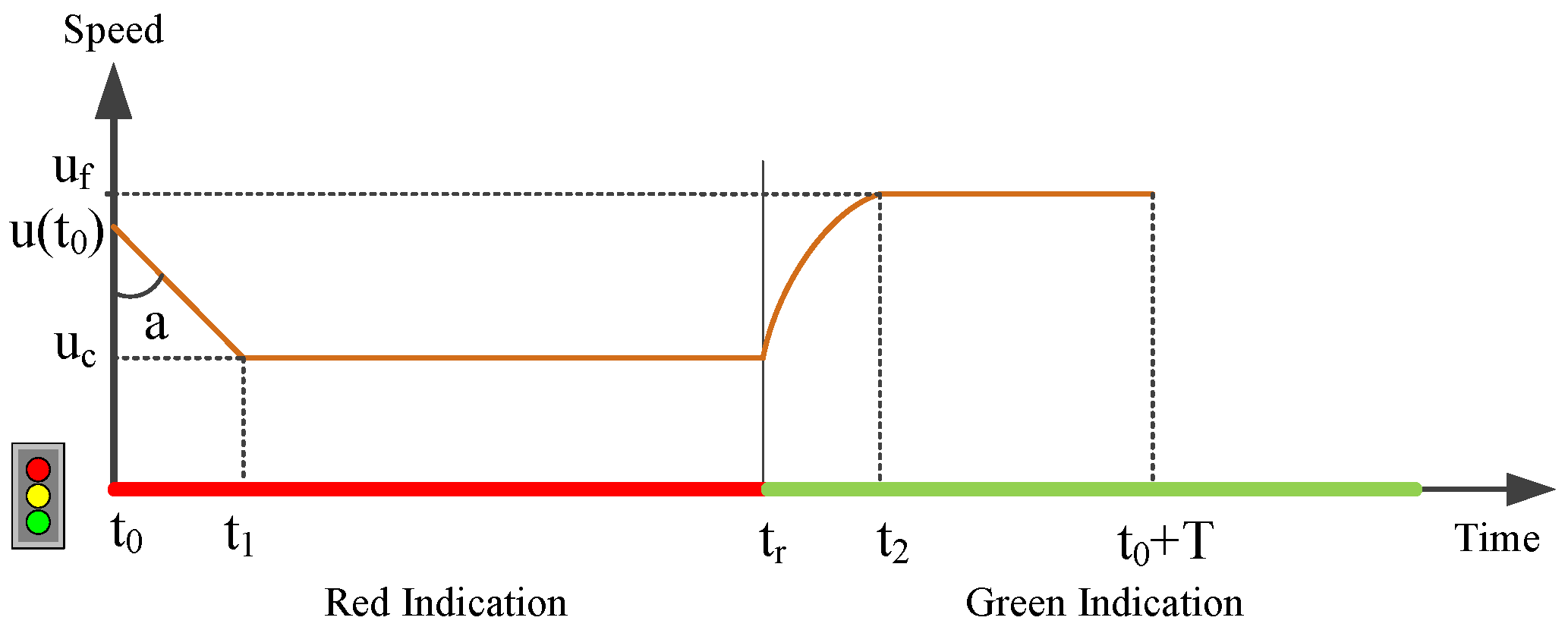
2.2. GLOSA for Buses

A simple bus fuel consumption model was developed and calibrated in [24,25]. The framework of the Virginia Tech Comprehensive Power-based Fuel Consumption Model (VT-CPFM), which was originally developed for LDVs, was used to develop the fuel model for buses as presented in Equation (8). The vehicle power used in the fuel model can be computed as Equation (9).

$$FC\left(t\right):\left\{\begin{array}{cc}{a}_0+a_{1}P\left(t\right)+a_{2}P{\left(t\right)}^2,& P\left(t\right)\ge 0\\ a_0& P\left(t\right)<0\end{array}\right.$$

(8)

$$P\left(t\right)=\left(\frac{R\left(t\right)+\left(1+\lambda +0.0025\xi u{\left(t\right)}^2\right)ma\left(t\right)}{3600{\eta }_{\mathrm{d}}}\right)·u\left(t\right)$$

(9)

where FC(t) denotes the instantaneous fuel consumption rate; ${\mathsf{\alpha }}_0$, ${\mathsf{\alpha }}_1$ and ${\mathsf{\alpha }}_2$ are the model coefficients for a specific vehicle type, which need to be calibrated for each vehicle; $\lambda$ is the mass factor accounting for rotational masses, a value of 0.1 is used for HDVs [30]; $\xi$ is the term related to gear ratio, which is assumed to be zero due to the lack of gear data; a(t) is the instantaneous acceleration level; R(t) is the resistance forces on the vehicle as given by Equation (4).

A regression-based approach was developed in [24] to calibrate the VT-CPFM model for buses. Mass field data, including instantaneous vehicle speed, fuel consumption rate, latitude, longitude, and altitude, were collected by test driving the buses around the town of Blacksburg, VA. In order to cover a wide range of real-world driving conditions, the test-driving routes consisted of two roadway sections: US 460 business (highway with a speed limit of 65 mph) and local streets (with a speed limit ranging from 25 to 45 mph). The collected data were divided into two datasets for the test bus. The first dataset was used for calibration purposes, and included 60% to 70% percent of the entire data for the test bus, and the remaining dataset was used for model validation. The regression-based model fitting can estimate the values of parameters ${\mathsf{\alpha }}_0$, ${\mathsf{\alpha }}_1$ and ${\mathsf{\alpha }}_2$ in Equation (8). The calibrated bus fuel model was compared with the measurement data and presented very good fitting accuracy, as shown in Figure 2.

3. Case Study

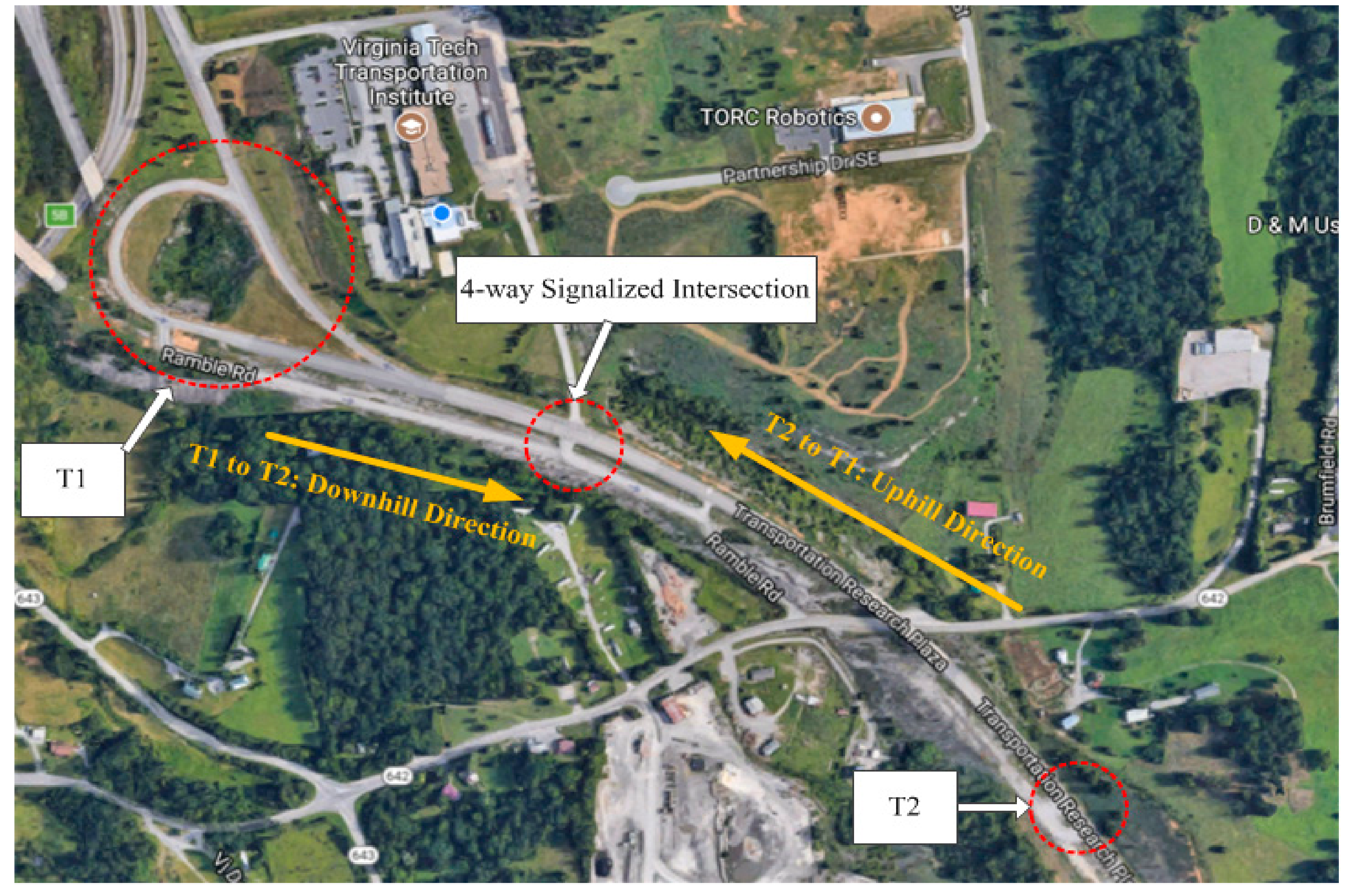
3.1. Test Environment

The connected vehicle testbed located at the Virginia Tech Transportation Institute (VTTI)’s Smart Road was used to validate the performance of the proposed B-GLOSA system. The Smart Road at VTTI is a 3.5 km (2.2-mile) roadway with turnaround loops at both ends. Wireless roadside equipment units are installed at spacing of around 500–600 m, which provides 5.9 GHz of short-range wireless communications between the infrastructure and vehicles. Two mobile roadside equipment sites are also available at the Smart Road. The Signal Phasing and Timing (SPaT) information at intersections can be remotely controlled by vehicle location or user input through wireless communication. The layout of the test road is illustrated in Figure 3. The upstream and downstream roadway connected by the signalized intersection is a surface roadway with two lanes, and each direction is a one lane road. Figure 3 shows that a four-way signalized intersection is located in the center. The roadway grades are approximately −3 percent for the downhill direction and +3 percent for the uphill direction. The stop lines for both directions are located on the signalized intersection. The B-GLOSA system is enabled when the bus is 200 m upstream of the stop bar and is disabled when the bus is 200 m downstream of the stop bar. Thus, both d_up and d_down are equal to 200 m. During the test drive in the uphill direction, the bus can accelerate up to 32–34 mph before merging to turnaround 1 if the bus was fully stopped at the intersection. Therefore, the speed limit was set as 30 mph. In order to have a fair comparison across different runs, buses attempted to drive at 30 mph before entering and after leaving the control range. Thus, two cones were placed at 200 m upstream (the first cone) and 200 m downstream (the second cone) of the intersection in each direction; thus, in total there were four cones, past which drivers were asked to drive at 30 mph.

In order to test the impact of different signal timing plans on the B-GLOSA system performance, four different signal timings were used during the test. Here, the variable is called “red offset”, which represents the remaining red offset time when the vehicle enters the test area by passing the first cone. We used four combinations of red offsets, namely 10, 15, 20 and 25 s. During the test, the testing bus is initially far away and driving to the downstream traffic signal, and the traffic signal shows a constant red indication. When the testing bus is passing the upstream location d_up, the countdown of the red offset (the remaining red indication time) is triggered by a random value from 10, 15, 20 or 25 s. Moreover, the upcoming green indication time is set as 25 s to ensure the bus can arrive at the downstream location, even if the bus is completely stopped at the signalized intersection.

In total, 30 participants were recruited to conduct the field test. All the participants were voluntarily recruited from BT bus drivers, since the test vehicle was a diesel bus provided by Blacksburg Transit (BT) and BT’s policy requires that the bus can be only operated by BT bus drivers. Each participant was asked to conduct three different driving scenarios, namely: (1) scenario 1—uninformed drive; (2) scenario 2—informed drive with signal timing; (3) scenario 3—informed drive with recommended speed. The aim of the field test was to investigate the impacts of road grades and red offset timings on vehicle performances, and the details of experimental design and statistical analysis are described in the next section. Each participant drove the test bus eight times for each driving direction, and the red offset value for each repeated trip was randomly selected from 10, 10, 15, 15, 20, 20, 25, 25 s, which means each predefined red offset value was repeated twice. In addition, each participant drove under the three different scenarios described below, under dry road surface and daylight conditions. In this way, each participant made 16 trips for each scenario (48 trips for three scenarios). The total trip number for 30 participants was 1440. Note that we only extracted the vehicle data for each trip by passing from the upstream location d_up to the downstream location d_down. Eventually, 1440 sets of trip information were collected as the raw dataset to analyze the system performance in the field test.

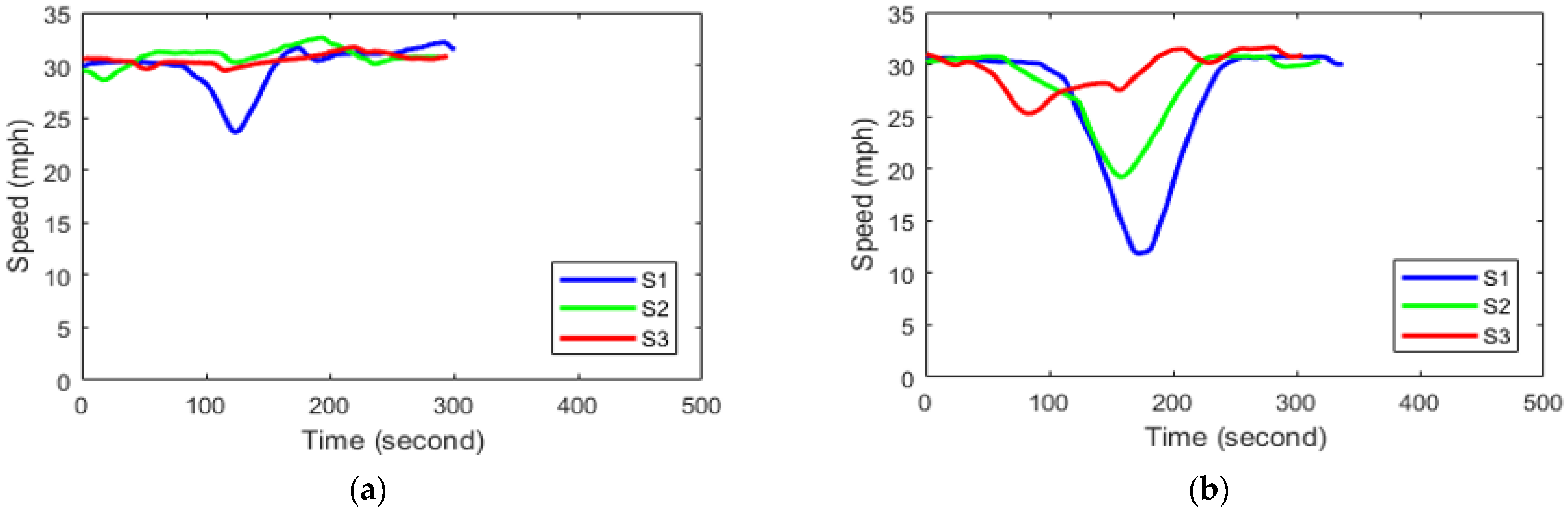
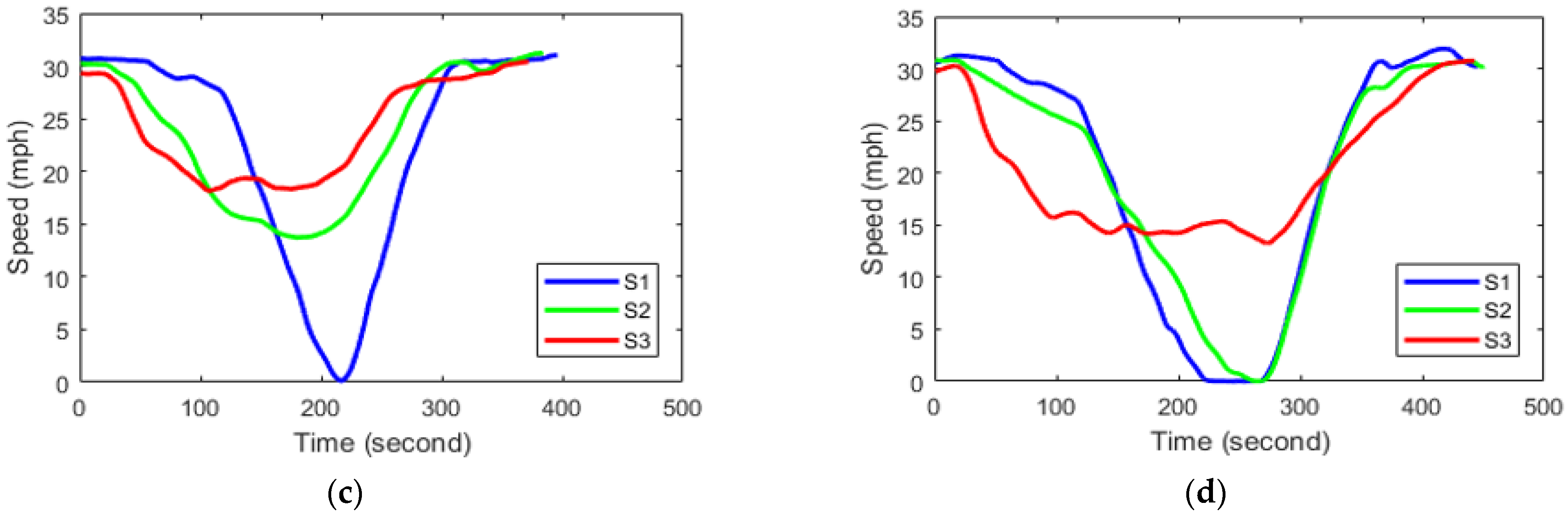
• Scenario 1 (S1)—Uninformed drive:

The driver needs to operate the bus normally by following traffic signal indications, without any driving assistant systems.

• Scenario 2 (S2)—Informed drive with the provision of signal timing information:

Via audio, when approaching the signalized intersection, the driver is provided information about when the traffic signal will turn green. The audio information provides a countdown of the signal timing to the next signal phase, which is used to assist the driver to perform the vehicle maneuver to traverse the intersection.

• Scenario 3 (S3)—Informed drive with recommended speed (B-GLOSA):

The driver is provided with audio information with the recommended speed when approaching the signalized intersection. The driver is asked to try his/her best effort to follow the recommended speed and adjust the vehicle speed accordingly.

A diesel-powered bus from BT was used in the field test, and the vehicle’s onboard units of our developed bus GLOSA system were installed in the cabinet control box behind the driver’s seat, as presented in Figure 4. The test bus was a 2014 New Flyer XD40 model with a 280-horsepower diesel engine. A differential GPS device was installed on the vehicle’s front top area to ensure the vehicle could receive accurate location information. A data acquisition system (DAS) customized by VTTI was installed in the control box, which collects GPS data, vehicle data, and SPaT, and communicates with a portable laptop to compute the recommended speed. All the test data were encrypted and stored in a hard drive disk, which were uploaded to the VTTI data service after completing the test. An audio system was chosen for conveying the information in the cases of scenario 2 and 3 because previous research [31,32] proved that visual displays can be highly distracting for the driver. In order to ensure that the proposed system can be used for real-time applications, the B-GLOSA system computes the optimum speed profile at 10 Hz, which means the optimum speed is recalculated every 0.1 s. The average driver’s perception reaction time was considered to be approximately 1.5 s. The communication system was tested, and we obtained around 0.5 s of latency. Hence, the audio system was preset to convey the information to the driver at intervals of 2 s.

3.2. Experimental Design and Statistical Analysis

The aim of the case study was to investigate the impact of three factors—scenario, road grade, and red indication offset—on trip fuel consumption level and travel time. Different experimental design approaches were considered for planning this case study so that the data obtained could be analyzed to yield valid and objective conclusions. The simplest option is that each factor could be randomly assigned for each testing trip when a participant passes the signalized intersection from upstream to downstream. However, practically there were several reasons why we could not conduct the field test in this way. Firstly, we did not want a participant to start with scenario 3 before the other two scenarios, since it is highly probable that a participant’s driving behavior for scenarios 1 or 2 will be changed after the experience of following the optimal speed profile in scenario 3. Secondly, testing the same road grade in two consecutive trips is not effective from a cost and time perspective. Given that the test site is a loop road starting from turnaround 2 to 1 and eventually returning to turnaround 2, participants needed to drive two loops to allow us to test two 3% (or −3%) runs. However, participants only needed to drive one loop to test a 3% uphill run followed by a −3% downhill run. Therefore, two factors (scenario and road grade) could not be randomized in this experiment. Specifically, each participant was required to start with scenario 1, followed by scenario 2, and lastly scenario 3. The road grade iterates through 3% uphill and −3% downhill by driving along the loop road. The only factor that could be randomized was the red indication offset at the instant the bus is 200 m upstream of the intersection.

Because the two factors are difficult to change, the split-split-plot design was used in this study. The split-split-plot design is a type of restricted randomization experimental design that was originally proposed in the field of agriculture to make the experiment design easier and more cost and time effective [33]. The split-split-plot design in this study was a blocked experiment with three levels of experimental units, as shown in Figure 5. The first level of the experimental units is the whole plot (scenario); the second level is the experimental units within the whole plot, called the split-plot (road grade); and the third level is the experimental units within the split-plot, called the split-split-plot (red indication offset). The red indication offset was the only factor that could be randomized without any effects on the experiment. Given that we had a limited participant pool and all the drivers were bus drivers from Blacksburg Transit, we did not recruit participants by gender or age groups. The participant effect (variation of driver behavior among participants) was considered to be a random effect, so it was not used as a fixed effect factor.

The JMP statistical software was used to analyze the split-split-plot experiment results. The results of fixed effect tests from the output of the Fit Mixed report are presented in

Table 1. Results of fixed effect tests.

Response Variable	Source	DF	DFDen	F Ratio	p Value
Fuel Consumption	Scenario	2	146	83.004	<0.0001
	Red offset	3	1255	1182.769	<0.0001
	Grade	1	175	7355.448	<0.0001
	Scenario*Grade	2	175	10.658	0.1872
	Scenario*Red offset	6	1255	12.449	0.0685
	Red offset*Grade	3	1255	30.084	<0.0001
	Scenario*Red offset*Grade	6	1255	8.796	0.1236
Travel Time	Scenario	2	146	660.503	<0.0001
	Red offset	3	1255	8623.917	<0.0001
	Grade	1	175	131.278	0.0853
	Scenario*Grade	2	175	13.477	0.0762
	Scenario*Red offset	6	1255	53.352	0.1082
	Red offset*Grade	3	1255	0.900	0.4849
	Scenario*Red offset*Grade	6	1255	3.029	0.6215

, which includes the degrees of freedom, F ratio, and p value from the ANOVA test. However, an ANOVA test can only determine if the results are significant overall. To further investigate which pairs of compositions from all the source factors have a significant difference, the Tukey test (also called Tukey’s Honest Significant Difference test) was used to compare all possible pairs of means [34]. For the response variable of fuel consumption, the test results indicated that S1 and S3 were significantly different for both uphill and downhill directions for various red indication offset values. Moreover, the differences between S1 and S2 were statistically significant, except for the cases of driving towards downhill direction with 20 and 25 s offset. In addition, the results showed that S2 and S3 were significantly different, except for the cases with a 10 s offset for both the uphill and downhill directions of travel.

In the table above, the “*” means multiple variables are included in the Source. Compared to the Tukey test results for the response variable of fuel consumption, using the response of travel during the test showed slightly different results. The differences between S1 and S3 were statistically significant, except for the cases with a 10 s red indication offset for both uphill and downhill directions, and driving with a 25 s red offset for the uphill direction. Moreover, S1 and S2 were only significantly different under 15 and 20 s red offsets for the uphill direction. For the uphill direction, the differences between S2 and S3 were statistically significant, except for the 10 s red offset. For downhill direction, the differences between S2 and S3 were statistically significant only when driving under a 15 s red offset. The test results demonstrated that the proposed B-GLOSA system produces a significantly different fuel consumption performance compared with S1 and S2 in most cases, by taking similar (or shorter) travel times. The quantitative performance analysis of the field test is presented as below.

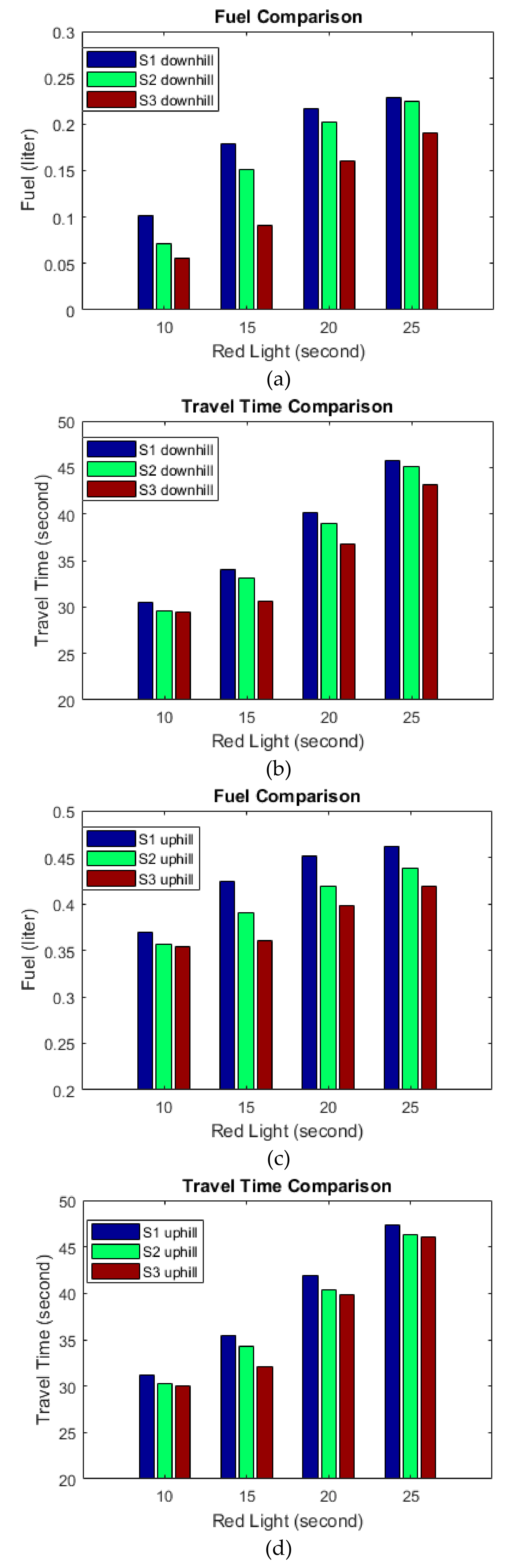
3.3. Quantitative Performance Analysis

The instantaneous fuel consumption, vehicle speed, and location were collected during each trip to calculate the average fuel consumption and travel times.

Table 2. Average trip fuel consumption (FC) levels.

Direction	Red Offset (Sec)	Scenario 1 FC (Liter)	Scenario 2 FC (Liter)	Scenario 3 FC (Liter)	Difference between S2 and S1 (%)	Difference between S3 and S1 (%)
Downhill	10	0.102	0.072	0.056	−29.7%	−44.9%
	15	0.179	0.151	0.091	−15.3%	−49.1%
	20	0.217	0.202	0.161	−6.7%	−25.8%
	25	0.229	0.224	0.190	−2.1%	−16.8%
Uphill	10	0.369	0.356	0.354	−3.5%	−4.2%
	15	0.424	0.390	0.360	−8.0%	−15.1%
	20	0.451	0.419	0.399	−7.1%	−11.6%
	25	0.462	0.438	0.419	−5.3%	−9.3%
Downhill Average		0.182	0.162	0.125	−13.4%	−34.2%
Uphill Average		0.427	0.401	0.383	−6.0%	−10.1%
Total Average		0.304	0.282	0.254	−9.7%	−22.1%

presents the average fuel consumption levels for one trip (from 200 m upstream to 200 m downstream) for different scenarios (1, 2, and 3), road grade (3% and −3%) and red offset time (10, 15, 20, 25 s). Under the same road grade and red offset time, the fuel consumption levels continued to decrease from scenarios 1 to 3, as presented in the left bar charts in Figure 6. Compared to scenario 1, scenario 2 consumed an average of 13.4% and 6.0% less fuel for the downhill and uphill directions, respectively. Compared to scenario 1, scenario 3 consumed an average of 34.2% and 10.1% less fuel for the downhill and uphill directions. Note that scenario 3 a produced significant amount of fuel savings (2.55 times the savings of scenario 2) under the downhill direction. It should be noted that 15 s of red offset corresponds to the maximum fuel savings (49.1% and 15.1%) for scenario 3 under both uphill and downhill directions. This result occurred because the bus equipped with the proposed B-GLOSA system showed the maximum speed difference compared to the case of the bus without B-GLOSA. Under the case of a 15 s red offset, drivers expect to stop when the vehicle is very close to the intersection since the signal turns from red to green at the last moment. In scenario 1, drivers usually start to reduce speed quickly when the vehicle is around 50 m away from the intersection, which results in a vehicle speed of 10–15 mph at the start of the green light. However, in scenario 3, the B-GLOSA system asks drivers to slow down to around 25 mph at the beginning, which results in a vehicle speed of greater than 25 mph at the start of the green light. Consequently, the average bus speed in scenario 3 was much higher than the speed in scenario 1 for the 15 s red interval offset, which resulted in the maximum savings of fuel. It is also very interesting to see that the test bus under the 3% uphill direction consumed 2–3 times the fuel compared to driving with a similar speed under the −3% downhill direction. In total, scenario 3 produced 22.1% of overall average fuel savings compared with scenario 1, and scenario 2 produced 9.7% of overall fuel savings. These high fuel saving rates achieved in scenario 3 proved that the proposed B-GLOSA system can efficiently save bus fuel in the vicinity of signalized intersections.

Table 3. Average trip travel times.

Direction	Red Offset (Sec)	Scenario 1 TT (Sec)	Scenario 2 TT (Sec)	Scenario 3 TT (Sec)	Difference between S2 and S1 (%)	Difference between S3 and S1 (%)
Downhill	10	30.4	29.6	29.4	−2.9%	−3.3%
	15	34.1	33.1	30.6	−2.8%	−10.1%
	20	40.1	39.0	36.7	−2.9%	−8.5%
	25	45.7	45.1	43.1	−1.4%	−5.6%
Uphill	10	31.1	30.2	30.0	−2.9%	−3.5%
	15	35.5	34.3	32.0	−3.3%	−9.7%
	20	42.0	40.3	39.9	−3.9%	−5.0%
	25	47.3	46.4	46.0	−2.0%	−2.7%
Downhill Average		37.6	36.7	35.0	−2.5%	−6.9%
Uphill Average		39.0	37.8	37.0	−3.0%	−5.3%
Total Average		38.3	37.2	36.0	−2.8%	−6.1%

presents the average trip travel times under different scenarios, grades, and red offset times. Under the same road grade and red offset time, a similar trend in which travel times continued to reduce from scenarios 1 to 3 can be observed in the right bar charts in Figure 6, which means scenario 3 always produced the least fuel consumption levels and travel times. Compared to scenario 1, scenario 2 required an average of 2.5% and 3.0% shorter travel times for downhill and uphill directions, respectively. Compared to scenario 1, scenario 3 required an average of 6.9% and 5.3% shorter travel times for downhill and uphill directions, respectively. Note that travel times under the uphill direction were not significantly different from those of the downhill direction. In total, scenario 3 produced 6.1% of overall average travel time savings compared with scenario 1, and scenario 2 produced 2.8% of overall travel time savings. The test results in Table 1 and Table 2 prove that the proposed bus GLOSA system can efficiently reduce fuel savings while also achieving a reasonable amount of travel time savings.

Sample vehicle speed profiles of a selected participant for downhill direction under various red offset timings are presented in Figure 7. All speed profiles have the similar starting and ending speeds of around 30 mph; thus, the comparisons between different scenarios are fair because the vehicle speed values between the start and end were affected by the settings of uninformed or informed driving in each scenario. For scenario 1, it can be observed that the vehicle came to a complete stop for the 20 and 25 s red offsets. Scenario 2 also had a complete stop under the 25 s red offset. Apparently, scenario 3 produced much smoother speed profiles compared with the other scenarios. The sample speed profiles demonstrated the benefits of the bus GLOSA system by helping the bus to drive smoothly to pass signalized intersections, and simultaneously reduce fuel consumption rates and travel times.

4. Conclusions

This study proposed a bus eco-driving system, entitled B-GLOSA. The developed system computes the fuel-efficient trajectory of buses using traffic signal data received from downstream signalized intersections. The key features of the proposed system are summarized below.

• A fuel consumption model for diesel buses was used in the proposed system to compute instantaneous fuel consumption rates, because this model is easy to calibrate using easy-to-access bus data.
• The vehicle dynamics model, fuel consumption model, signal timings, and vehicle speed and distance relationship are used to construct an optimization problem.
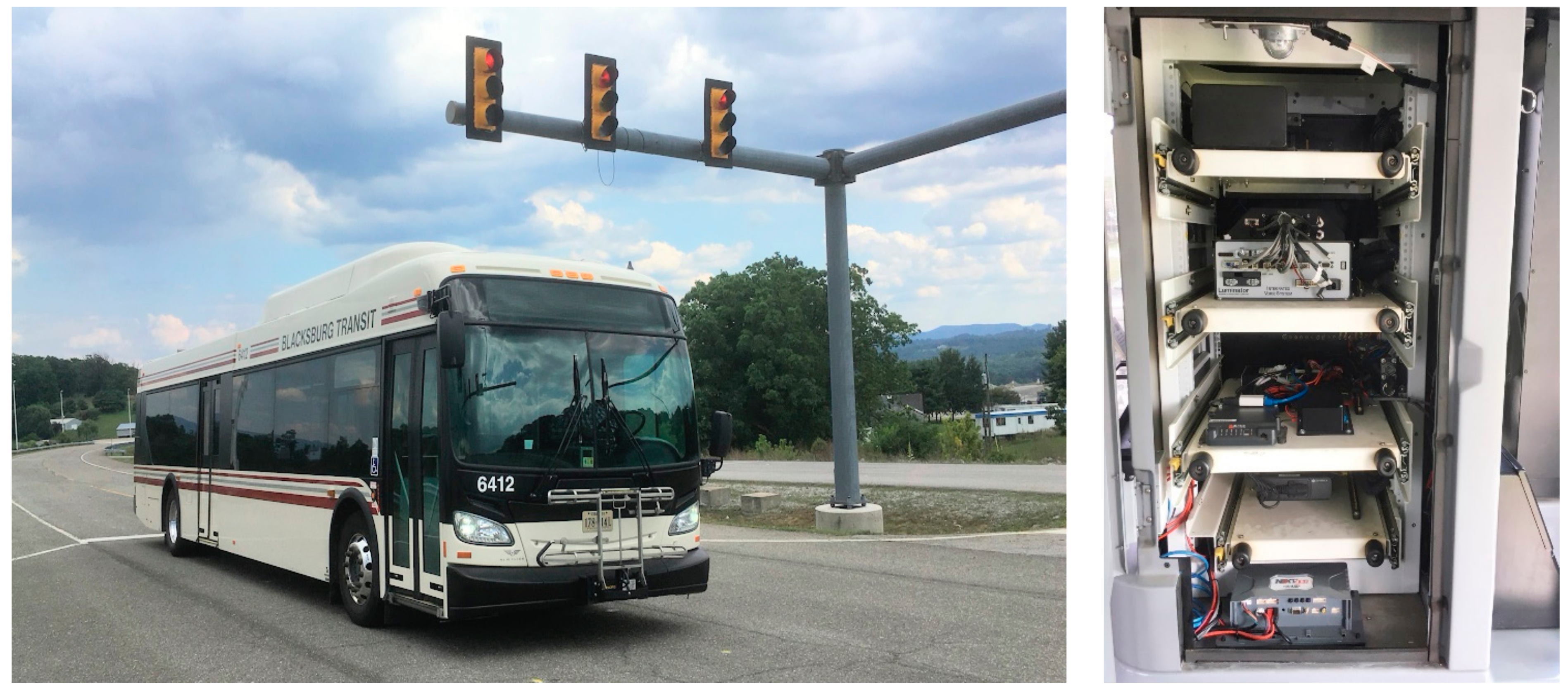
• A moving-horizon dynamic program and an A-star algorithm is used to solve the optimization problem and calculate the energy-optimized vehicle trajectory to assist buses to proceed through signalized intersections efficiently. The proposed B-GLOSA system was implemented and field tested to validate the real-world benefits. The test results and the recommendations for future research are summarized below.
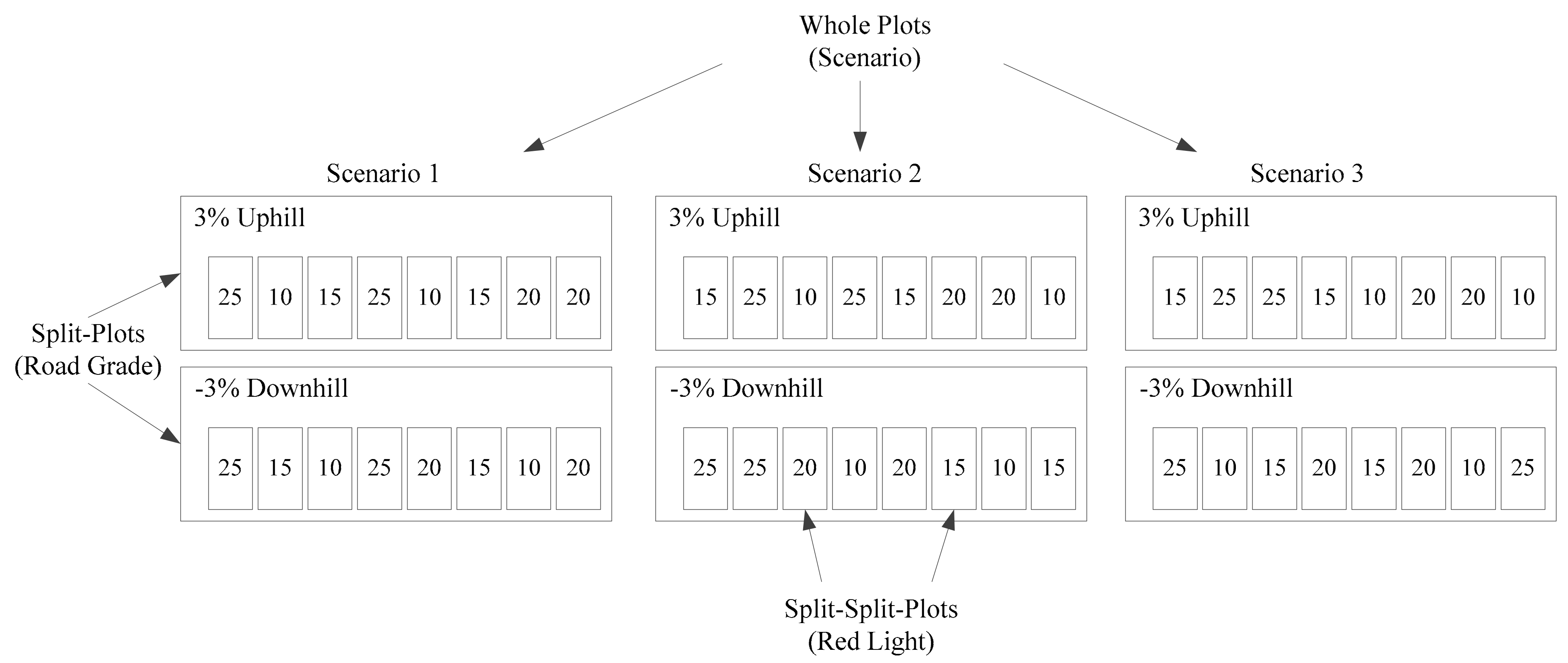
• The Virginia Smart Road test facility was used to conduct the field test using 30 participants. A split-split-plot experimental design was used to test the developed B-GLOSA system for different impact factors of road grades and red indication offsets, and statistical analysis was conducted to demonstrate that the fuel consumption performances were significantly different among three test scenarios.
• The quantitative analysis of the test results demonstrated that the proposed B-GLOSA system can greatly smooth the bus trajectory while traversing a signalized intersection, and simultaneously save fuel consumption and travel times.
• Compared to the uninformed drive, the test results demonstrated that the B-GLOSA can efficiently reduce fuel consumption by 22.1% and simultaneously reduce vehicle travel times by 6.1%.
• In future research, the B-GLOSA system will be tested within a microscopic simulation environment to quantify he network-level impact for various traffic conditions and heterogeneous traffic including LDVs and buses.

References

1. Barth, M.; Boriboonsomsin, K. Real-World Carbon Dioxide Impacts of Traffic Congestion. Transp. Res. Rec. J. Transp. Res. Board 2008, 2058, 163–171. [Google Scholar] [CrossRef] [Green Version]
2. Rakha, H.; Ahn, K.; Trani, A. Comparison of MOBILE5a, MOBILE6, VT-MICRO, and CMEM models for estimating hot-stabilized light-duty gasoline vehicle emissions. Can. J. Civ. Eng. 2003, 30, 1010–1021. [Google Scholar] [CrossRef]
3. Mahler, G.; Vahidi, A. Reducing idling at red lights based on probabilistic prediction of traffic signal timings. In Proceedings of the 2012 American Control Conference (ACC), Montreal, QC, Canada, 27–29 June 2012; IEEE: Piscataway, NJ, USA, 2012; pp. 6557–6562. [Google Scholar]
4. Kamalanathsharma, R.K.; Rakha, H.A.; Yang, H. Networkwide Impacts of Vehicle Ecospeed Control in the Vicinity of Traffic Signalized Intersections. Transp. Res. Rec. J. Transp. Res. Board 2015, 2503, 91–99. [Google Scholar] [CrossRef]
5. Ahn, K.; Rakha, H.A. Network-wide impacts of eco-routing strategies: A large-scale case study. Transp. Res. Part D Transp. Environ. 2013, 25, 119–130. [Google Scholar] [CrossRef]
6. Abdelghaffar, H.M.; Rakha, H.A. A Novel Decentralized Game-Theoretic Adaptive Traffic Signal Controller: Large-Scale Testing. Sensors 2019, 19, 2282. [Google Scholar] [CrossRef] [PubMed] [Green Version]
7. Saboohi, Y.; Farzaneh, H. Model for optimizing energy efficiency through controlling speed and gear ratio. Energy Effic. 2008, 1, 65–76. [Google Scholar] [CrossRef]
8. Saboohi, Y.; Farzaneh, H. Model for developing an eco-driving strategy of a passenger vehicle based on the least fuel consumption. Appl. Energy 2009, 86, 1925–1932. [Google Scholar] [CrossRef]
9. Barth, M.; Boriboonsomsin, K. Energy and emissions impacts of a freeway-based dynamic eco-driving system. Transp. Res. Part D Transp. Environ. 2009, 14, 400–410. [Google Scholar] [CrossRef]
10. Malakorn, K.J.; Park, B. Assessment of mobility, energy, and environment impacts of IntelliDrive-based Cooperative Adaptive Cruise Control and Intelligent Traffic Signal control. In Proceedings of the 2010 IEEE International Symposium on Sustainable Systems and Technology (ISSST), Arlington, VA, USA, 17–19 May 2010; IEEE. [Google Scholar]
11. Kamalanathsharma, R.K.; Rakha, H.A. Agent-Based Simulation of Ecospeed-Controlled Vehicles at Signalized Intersections. Transp. Res. Rec. J. Transp. Res. Board 2014, 2427, 1–12. [Google Scholar] [CrossRef]
12. Asadi, B.; Vahidi, A. Predictive Cruise Control: Utilizing Upcoming Traffic Signal Information for Improving Fuel Economy and Reducing Trip Time. IEEE Trans. Control Syst. Technol. 2010, 19, 707–714. [Google Scholar] [CrossRef]
13. Guan, T.; Frey, C.W. Predictive fuel efficiency optimization using traffic light timings and fuel consumption model. In Proceedings of the 16th International IEEE Conference on Intelligent Transportation Systems (ITSC 2013), The Hague, The Netherlands, 6–9 October 2013; IEEE: Piscataway, NJ, USA, 2013; pp. 1553–1558. [Google Scholar]
14. Fadzir, T.M.A.M.; Mansor, H.; Gunawan, T.S.; Janin, Z. Development of School Bus Security System Based on RFID and GSM Technonologies for Klang Valley Area. In Proceedings of the 2018 IEEE 5th International Conference on Smart Instrumentation, Measurement and Application (ICSIMA), Songkhla, Thailand, 28–30 November 2018; IEEE: Piscataway, NJ, USA, 2018; pp. 1–5. [Google Scholar]
15. Witten, T.; Samuel, A.; Guerrero, I.; Alden, A.; Rakha, H.; Wang, J.; Chen, H.; Mayer, B.; Edwards, A.; Connell, C.; et al. Transit Bus Routing On-Demand Developing an Energy-Saving System. 2015, Report No. 0704-0188, Federal Transit Administration. Available online: https://ridebt.org/images/documents/TIGGER-FINAL-REPORT.pdf (accessed on 8 December 2021).
16. Nguyen, T.; Nguyen-Phuoc, D.Q.; Wong, Y.D. Developing artificial neural networks to estimate real-time onboard bus ride comfort. Neural Comput. Appl. 2021, 33, 5287–5299. [Google Scholar] [CrossRef]
17. Zhang, L.; Liang, W.; Zheng, X. Eco-Driving for Public Transit in Cyber-Physical Systems Using V2I Communication. Int. J. Intell. Transp. Syst. Res. 2018, 16, 79–89. [Google Scholar] [CrossRef]
18. Bagherian, M.; Mesbah, M.; Ferreira, L. Using Vehicle to Infrastructure Communication to Reduce Bus Fuel Consumption at Intersections. In Proceedings of the 95th Annual Meeting Transportation Research Board, Washington, DC, USA, 10–14 January 2016. [Google Scholar]
19. Chen, H.; Rakha, H.A.; Almanna, M.; Loulizi, A.; El-Shawarby, I. Field Implementation of an Eco-cooperative Adaptive Cruise System at Signalized Intersections. In Proceedings of the 96th Annual Meeting Transportation Research Board, Washington, DC, USA, 8–12 January 2017. [Google Scholar]
20. Rakha, H.A.; Chen, H.; Almanna, M.; Kamalanathsharma, R.K.; Loulizi, A.; El-Shawarby, I. Field Testing of Eco-Speed Control Using V2I Communication: Report No. 54-6001805, Connected Vehicle/Infrastructure University Transportation Center, U.S. Department of Transportation (CVI-UTC). 2016. Available online: https://cvi-utc.org/wp-content/uploads/2015/10/Rakha_Field-Testing-of-Eco-Speed-Control-Using-V2I-Communication_Final.pdf (accessed on 8 December 2021).
21. Almannaa, M.H.; Chen, H.; Rakha, H.A.; Loulizi, A.; El-Shawarby, I. Reducing Vehicle Fuel Consumption and Delay at Signalized Intersections: Controlled-Field Evaluation of Effectiveness of Infrastructure-to-Vehicle Communication. Transp. Res. Rec. J. Transp. Res. Board 2017, 2621, 10–20. [Google Scholar] [CrossRef]
22. Qi, X.; Wu, G.; Barth, M.J.; Boriboonsomsin, K.; Wang, P. Energy Impact of Connected Eco-driving on Electric Vehicles. In Road Vehicle Automation 4, 2nd ed.; Beiker, S., Gereon, M., Eds.; Springer: New York, NY, USA, 2017; Volume 4, pp. 97–111. [Google Scholar]
23. Katsaros, K.; Kernchen, R.; Dianati, M.; Rieck, D. Performance study of a Green Light Optimized Speed Advisory (GLOSA) application using an integrated cooperative ITS simulation platform. In Proceedings of the 2011 7th International Wireless Communications and Mobile Computing Conference, Istanbul, Turkey, 4–8 July 2011; IEEE: Piscataway, NJ, USA, 2011; pp. 918–923. [Google Scholar]
24. Wang, J.; Rakha, H.A. Fuel consumption model for conventional diesel buses. Appl. Energy 2016, 170, 394–402. [Google Scholar] [CrossRef]
25. Wang, J.; Rakha, H.A. Convex Fuel Consumption Model for Diesel and Hybrid Buses. Transp. Res. Rec. J. Transp. Res. Board 2017, 2647, 50–60. [Google Scholar] [CrossRef]
26. Xia, H. Eco-Approach and Departure Techniques for Connected Vehicles at Signalized Traffic Intersections. Doctoral Dissertation, University of California, Oakland, CA, USA, 2014. Riverside. Available online: https://escholarship.org/uc/item/5xz408r4 (accessed on 8 December 2021).
27. Kamalanathsharma, R.K. Eco-Driving in the Vicinity of Roadway Intersections-Algorithmic Development, Modeling, and Testing. Doctoral Dissertation, Virginia Polytechnic Institute and State University, Blacksburg, VA, USA, 2014. Available online: https://vtechworks.lib.vt.edu/handle/10919/56987 (accessed on 8 December 2021).
28. Yu, K.; Yang, J.; Yamaguchi, D. Model predictive control for hybrid vehicle ecological driving using traffic signal and road slope information. Control Theory Technol. 2015, 13, 17–28. [Google Scholar] [CrossRef]
29. Zhang, Z.; Zhao, Z. A Multiple Mobile Robots Path planning Algorithm Based on A-star and Dijkstra Algorithm. Int. J. Smart Home 2014, 8, 75–86. [Google Scholar] [CrossRef] [Green Version]
30. Feng, C. Transit Bus Load-Based Modal Emission Rate Model Development. Science Inventory. Doctoral Dissertation, Georgia Institute of Technology, Atlanta, GA, USA, 2007. Available online: https://smartech.gatech.edu/handle/1853/14583 (accessed on 8 December 2021).
31. Young, K.; Lenné, M.G. Driver engagement in distracting activities and the strategies used to minimise risk. Saf. Sci. 2010, 48, 326–332. [Google Scholar] [CrossRef]
32. Stutts, J.; Feaganes, J.; Reinfurt, D.; Rodgman, E.A.; Hamlet, C.; Gish, K.; Staplin, L. Driver’s exposure to distractions in their natural driving environment. Accid. Anal. Prev. 2005, 37, 1093–1101. [Google Scholar] [CrossRef]
33. Jones, B.; Nachtsheim, C.J. Split-plot designs: What, why, and how. J. Qual. Technol. 2009, 41, 340–361. [Google Scholar] [CrossRef]
34. Abdi, H. Guttman scaling. Encycl. Res. Des. 2010, 2, 1–5. [Google Scholar]
Figure 1. The fuel-optimized vehicle trajectory.
Energies 15 01491 g001
Figure 2. Model validation for bus fuel consumption model.
Energies 15 01491 g002
Figure 3. Layout of the test road (source: Google Maps).
Energies 15 01491 g003
Figure 4. Hardware of the vehicle onboard units in the bus GLOSA system.
Energies 15 01491 g004
Figure 5. Structure of the split split plot design.
Energies 15 01491 g005
Figure 6. Comparison of test results for fuel levels and travel times: (a) fuel in downhill; (b) travel time in downhill; (c) fuel in uphill; (d) travel time in uphill.
Energies 15 01491 g006
Figure 7. Vehicle speed profiles of a selected participant for the downhill direction under various red offset timings: (a) 10 s; (b) 15 s; (c) 20 s; (d) 25 s.
Energies 15 01491 g007aEnergies 15 01491 g007b