Induction Motor Field-Oriented Sensorless Control with Filter and Long Cable

Abstract

In recent years, part of the efforts of the electric drive researcher has been focused on the study of sensorless control algorithms that allow controlling the machine without a speed measure and with ever-fewer measurement devices. This article proposes a possible solution for the submarine application of an asynchronous motor. The motor is designed to drive a petrol pump at a depth of three thousand meters. The motor is fed by an inverter that is located on an offshore platform, and they are connected through a filter and a cable that is 19.74 km long. In this application, it is not suitable to use a speed measurement device; in fact, at this depth it is important to use as few components as possible, in order to increase the system reliability. A control algorithm that only needs available electrical measures is proposed below.

1. Introduction

In recent decades, induction motor drives have established themselves in various applications where high reliability is required. In this paper, a submarine application of an induction motor is studied. The motor is used to drive a petrol pump far from the oil platform. In fact, in recent years, in order to increase plant productivity, instead of removing the platform when the oil field runs out, the oil companies use to keep the original platform and look for a new field nearby [1]. For this reason the motor and the pump are far away from the plant. Thus, the system under study is composed of an inverter connected to an induction machine through a filter and a long submarine cable [2,3]. The inverter and the filter are located on the oil platform while the motor and the pump are on the subsea oil exploitation, and they are connected through a 19.74 km cable. This system, analogous to what has been argued in [4], presents a series of challenges for the control system; first of all, the difficulty in carrying out measurements such as motor speed, stator current, and stator voltage. For this type of application, the state of the art involves the use of scalar control algorithms, as shown in [5], in order to avoid the use of motor realtime feedback. Scalar controls such as V/Hz methods are easy to implement and guarantee good steady-state response. However, open-loop control strategies have some drawbacks, such as slow dynamic behavior and robustness. In the past, many closed-loop control algorithms have been studied and proposed in the technical literature, such as Field-Oriented Control (FOC) and Direct-Torque Control (DTC). These control methods offer high precision and good dynamics; in particular, the FOC algorithm allows controlling separately the flux and the speed. However, these control strategies require accurate electrical and mechanical measurements.

In the discussion below, we will show how to obtain these variables starting from the available measures. Another challenge of this application is the parameter variation, such as cable resistance, inductance, capacitance, and induction machine rotor resistance, as shown in [6].

Furthermore, the cable generates a voltage drop which must be compensated for. In order to solve all these problems, a Sensorless Compensated Direct Field-Oriented Control (SCDFOC) method has been developed. The advantages of the proposed algorithm are several. First of all, it does not require any speed sensor, since the use of a speed sensor is not convenient for reliability reasons in submarine applications; in fact, a speed sensor requires maintenance for its correct functioning, and this is impossible due to the depth of sea considered in this application; the same considerations pertain to the other measurement systems. In addition, all the sensors that are installed on the motor should be maintainable and replaceable through the use of submarine robots. Secondly, the proposed algorithm only needs the electric measurements available on the offshore platform, any variable necessary for its functioning will be estimated or observed, thus reducing considerably the number of required sensors. In conclusion, the use of a Field Oriented Control method allows obtaining a more efficient speed control, and combined with the use of a Luenberger Observer for the induction machine, introduced in [7], it guarantees a better robustness to the parametric variations.

2. Direct Field-Oriented Control Theory

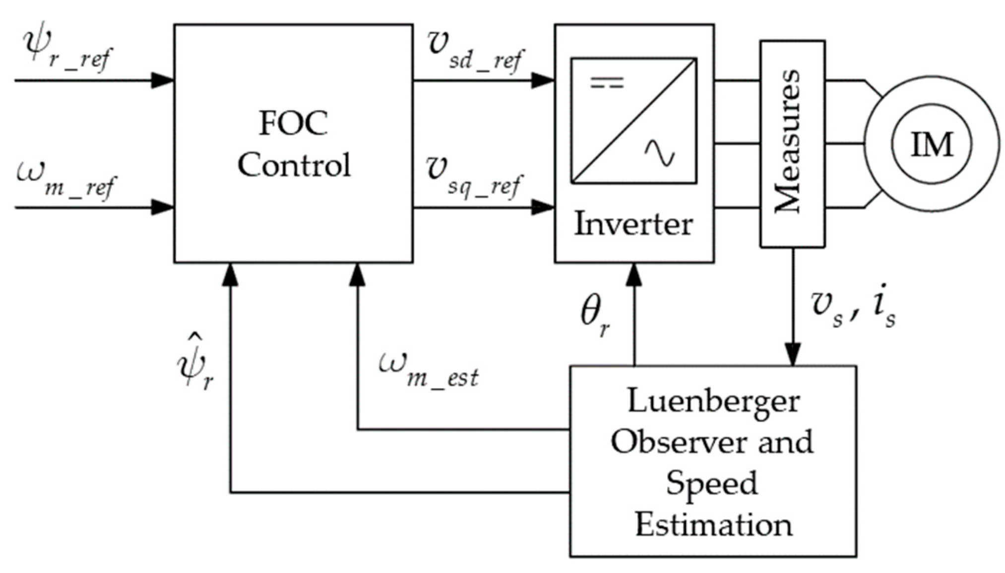
The control described below is used in a high-power application; so, efficiency becomes important for this type of system. To reach high efficiency a Direct Field-Oriented Control (DFOC) has been chosen for the application. This type of control also allows a fast and accurate response, as mentioned in [8]. Field-oriented control, also named vector control, was introduced at the beginning of 1970s, and it allows imitation of the DC motor performance considering a synchronous rotating reference frame. The reference is obtained applying the Park transformation, where the reference angle is the rotor flux angle. So, the rotor flux must be known, but since its measurement is difficult to attain, it is necessary to introduce a rotor flux observer that will be described in the next section. The outputs of the observer are the Rotor Flux module and angle. The angle is used for the orientation of all the electrical variables, and the module is compared to the rotor flux reference, which is the first reference of the DFOC. The second reference is the motor speed, which should be compared with the measured speed. In the application described below the speed measurement is not available; so, a speed estimation algorithm is introduced to estimate the speed value without using speed sensors, such as encoders or resolvers.

A diagram of the described control is shown in Figure 1.

The control works properly when the inverter is directly connected to the motor, but, in the studied application, the inverter is connected to the motor through a filter and a long submarine cable. In the following, an improvement for the DFOC control presented will be described and analyzed.

3. Motor Modeling and Luenberger Observer

The motor dynamic model is defined according to the usual α-β Clarke transformation, so a stationary reference frame is used for the motor dynamic modeling. In this paper, it will be assumed that the α-axis coincides with the real axis, and the β-axis coincides with the imaginary axis. Therefore, every electrical rotating vector can be expressed in terms of its components; for example, the stator flux can be expressed as follows:

$${\overline{\psi }}_s={\psi }_{s\alpha }+j{\psi }_{s\beta }$$

(1)

According to this symbology, the induction machine model is defined as follows:

$${\dot{\overline{\psi }}}_s=-\frac{R_s}{\Delta }(L_r{\overline{\psi }}_s-L_m{\overline{\psi }}_r)+{\overline{v}}_s$$

(2)

$${\dot{\overline{\psi }}}_r=-\frac{R_r}{\Delta }(L_s{\overline{\psi }}_r-L_m{\overline{\psi }}_s)+j\omega {\overline{\psi }}_r$$

(3)

$$\dot{\omega }=\frac{T_{em}-T_l}{J}\frac{P}{2}$$

(4)

$$T_{em}=\Im m({\overline{i}}_s\cdot {\overline{\psi }}_s^{*})$$

(5)

$${\overline{i}}_s=\frac{1}{\Delta }(L_r{\overline{\psi }}_s-L_m{\overline{\psi }}_r)$$

(6)

$${\overline{i}}_r=\frac{1}{\Delta }(L_s{\overline{\psi }}_r-L_m{\overline{\psi }}_s)$$

(7)

with

$$\Delta =L_r{L}_s-L_m^2$$

$$L_s=L_{ls}+L_m$$

$$L_r=L_{lr}+L_m$$

where the symbols are defined as:

•

$R_s,R_r$ stator and rotor resistance;

•

$L_s,L_r$ stator and rotor self-inductances;

•

$L_{ls},L_{lr}$ stator and rotor leakage inductances;

•

$L_m$ mutual inductance;

•

$J$ moment of inertia;

•

$P$ number of poles;

•

${\overline{\psi }}_{s,}{\overline{\psi }}_r$ stator and rotor flux vectors;

•

${\overline{i}}_s,{\overline{i}}_r$ stator and rotor current vector;

•

${\overline{v}}_s$ stator voltage;

•

$T_{em}$ electromagnetic torque;

•

$T_l$ load torque; and

•

$\omega$ angular rotor speed (expressed in electrical rad/s).

Starting from this model, it is possible to obtain a state observer, which can be derived from Equations (2)–(7) as follows:

$$\dot{\overline{\mathsf{\psi }}} = \mathrm{A} \overline{\mathsf{\psi }} + \overline{\mathrm{v}} + {\overline{\mathrm{e}}}_{mf}$$

(8)

$${\overline{\mathrm{i}}}_s=\mathrm{C} \overline{\mathsf{\psi }}$$

(9)

where:

$$\overline{\mathsf{\psi }}=\left[\begin{array}{l}{\overline{\psi }}_s\\ {\overline{\psi }}_r\end{array}\right],\hspace{0.17em}\hspace{0.17em}\hspace{0.17em}\hspace{0.17em}\hspace{0.17em}\hspace{0.17em} \overline{\mathrm{v}}=\left[\begin{array}{l}{\overline{v}}_s\\ 0\end{array}\right],\hspace{0.17em}\hspace{0.17em}\hspace{0.17em}\hspace{0.17em}\hspace{0.17em}{ \overline{\mathrm{e}}}_{mf}=\left[\begin{array}{c}0\\ j\omega {\overline{\psi }}_r\end{array}\right]$$

(10)

$$\mathrm{A}=\frac{1}{\Delta }\left[\begin{array}{cc}-R_s{L}_r& R_s{L}_m\\ R_r{L}_m& -R_r{L}_s+j\omega \Delta \end{array}\right],\hspace{0.17em}\hspace{0.17em}\hspace{0.17em}\hspace{0.17em}\hspace{0.17em}\hspace{0.17em}\hspace{0.17em}\mathrm{C}=\frac{1}{\Delta }\left[\begin{array}{cc}{L}_r& -L_m\end{array}\right]$$

(11)

The obtained model can be considered a linear system with a time-varying parameter $\omega$, as shown in Equations (7)–(9). It should be noted that $\omega$ has a dynamic slower than the other states variables; hence, its value can be considered as a constant.

As known, the system model already represents a state observer. However, its dynamics are too slow to be used in a control algorithm. Moreover, it is also well known that an observer obtained using only the motor model is affected by a certain error caused by the uncertainty of the motor parameters, it is necessary to introduce a system observer as studied in [7,8,9]. In fact, the motor parameters are affected primarily by measurement errors and parameter variations, mainly as a function of the temperature, especially affecting the rotor resistance in the case of induction machines. In addition, it is difficult to obtain the temperature measurement from the motor and estimate the rotor resistance. To compensate for these errors, a Luenberger feedback is introduced, which compares the measured stator currents with the observed ones, which are the output of the dynamic system, as shown in Equation (9). The error is then multiplied by a constant matrix $\mathrm{H}$ named the Luenberger Matrix; the result thus obtained is added into Equation (8) as follows:

$$\dot{\overline{\mathsf{\psi }}}=\mathrm{A} \overline{\mathsf{\psi }}+ \overline{\mathrm{v}}+{ \overline{\mathrm{e}}}_{mf}+\mathrm{H}({ \overline{\mathrm{i}}}_s-{ \widehat{\overline{\mathrm{i}}}}_s)$$

(12)

where ${\widehat{\mathrm{i}}}_s$ represents the estimated current vector, and the matrix $\mathrm{H}$ is defined in Equation (13).

$$\mathrm{H}=\left[\begin{array}{c}{K}_s\\ K_r\end{array}\right]$$

(13)

$K_s$ and $K_r$ represent the stator and rotor Luenberger gains, respectively. The observer can resist parametric variations; this is the main reason why the Luenberger observer was chosen for this application.

As known from classical control theory, to obtain a correct observer, the model of the system must be asymptotically stable and observable; meanwhile, the resulting observer must be stable. Induction motor model stability depends on the rotor speed values; however, it is equally well known that the motor is stable for most of the speed values. In addition, the observability of the system is guaranteed by matrices $\mathrm{C}$. For the observer stability, it is necessary to study the eigenvalues of the following matrix:

$${\mathrm{A}}_L=\mathrm{A}-\mathrm{HC}$$

(14)

The choice of the two gains $K_s$ and $K_r$ affects the stability of the observer; for this reason, an algorithm was developed to search for Luenberger gains as will be shown later in this paper.

4. Speed Estimation Algorithm

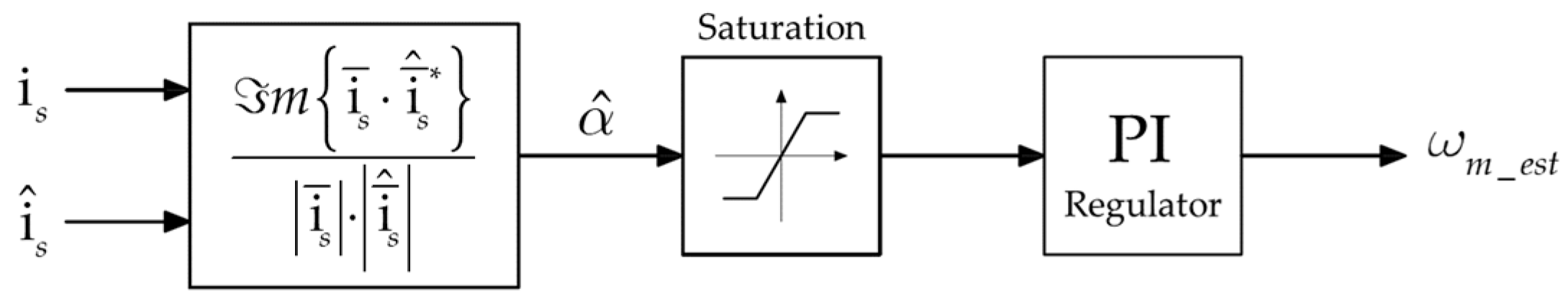
A speed estimation algorithm for an induction machine has already been discussed in [7], and it is shown in Figure 2. Measured stator currents and observed stator currents are compared using a vector product, as shown in Equation (15):

$$\widehat{\alpha }=\arcsin \left(\frac{\Im m\left\{{ \overline{\mathrm{i}}}_s\cdot {\widehat{\overline{\mathrm{i}}}}_s^{*}\right\}}{\left|{ \overline{\mathrm{i}}}_s\right|\hspace{0.17em}\cdot \hspace{0.17em}\left|{ \widehat{\overline{\mathrm{i}}}}_s\right|}\right)\cong \left(\frac{\Im m\left\{{ \overline{\mathrm{i}}}_s\cdot { \widehat{\overline{\mathrm{i}}}}_s^{*}\right\}}{\left|{ \overline{\mathrm{i}}}_s\right|\hspace{0.17em}\cdot \hspace{0.17em}\left|{ \widehat{\overline{\mathrm{i}}}}_s\right|}\right)$$

(15)

The term $\widehat{\alpha }$ is proportional to the speed variation, and it represents the acceleration of the machine. This variable can be integrated, and the estimated speed ${\omega }_{m\_est}$ can be obtained. When the two currents are equal the vectorial product is zero, but when a speed variation occurs, term $\widehat{\alpha }$ becomes different from zero, and the observed vector ${\widehat{\mathrm{i}}}_s$ is forced to follow the measured one. In order to improve the system stability at high speed and to obtain a faster response, a proportional gain is introduced, so $\widehat{\alpha }$ becomes the input of a PI regulator, as shown in Figure 2.

The presence of the denominator in Equation (15) means that the alpha signal can be subject to strong oscillations and pulses, which can affect the speed estimation. To eliminate these problems a saturation is introduced in the algorithm. Proportional and integral gains of the speed estimation are chosen empirically during the implementation of the simulations.

5. Luenberger Gains Determination

As already explained, to guarantee the stability of the Luenberger observer, the stability of matrix ${\mathrm{A}}_L$ is studied; in order to study the eigenvalues of the matrix it is necessary to rewrite the matrix decomposing the complex number. Matrix ${\mathrm{A}}_L$ thus obtained is written below.

$${\mathrm{A}}_L=\frac{1}{\Delta }\hspace{0.17em}\left[\begin{array}{cccc}-R_s{L}_r+K_s{L}_r& R_s{L}_m-K_s{L}_m& 0& 0\\ R_r{L}_m+K_r{L}_r& -R_r{L}_s-K_r{L}_m& 0& -\omega \Delta \\ 0& 0& -R_s{L}_r+K_s{L}_r& R_s{L}_m-K_s{L}_m\\ 0& \omega \Delta & R_r{L}_m+K_r{L}_r& -R_r{L}_s-K_r{L}_m\end{array}\right]$$

(16)

In this matrix, it is possible to observe all the machine parameters and also the machine speed. The latter is a variable quantity, so the eigenvalues will move in the Gauss plane during the operation of the machine. The algorithm chooses the Luenberger gains, imposing the nominal speed, and calculates the eigenvalues varying $K_s$ and $K_r$, verifying when they are on the left side of the imaginary axis. The output of the algorithm is a vector of possible Luenberger gains; the latter must be tested in simulations in order to verify their stability and choose the optimal ones.

The variation of the eigenvalues in function of speed can be studied imposing the Luenberger gains obtained with the previous process in the matrix and varying the speed.

The induction motor parameters are reported in

Table 1. Motor parameters.

	Parameter	Value
$P_n$	Rated output power	1.65 MW
$V_n$	Rated voltage	9840 V (∆)
$I_n$	Rated current	131.3 A
$C_p$	Pole pairs	1
${\omega }_n$	Rated speed	412.177 rpm
$T_n$	Rated torque	4009 Nm
$J$	Inertia	8.52 kgm2
$\cos \varphi$	Power factor	0.89
$R_s$	Stator resistance	42.7 mΩ
$R_r$	Rotor resistance	39.84 mΩ
$L_s$	Stator inductance	50.15 mH
$L_r$	Rotor inductance	49.64 mH
$L_m$	Magnetizing inductance	48.31 mH

below:

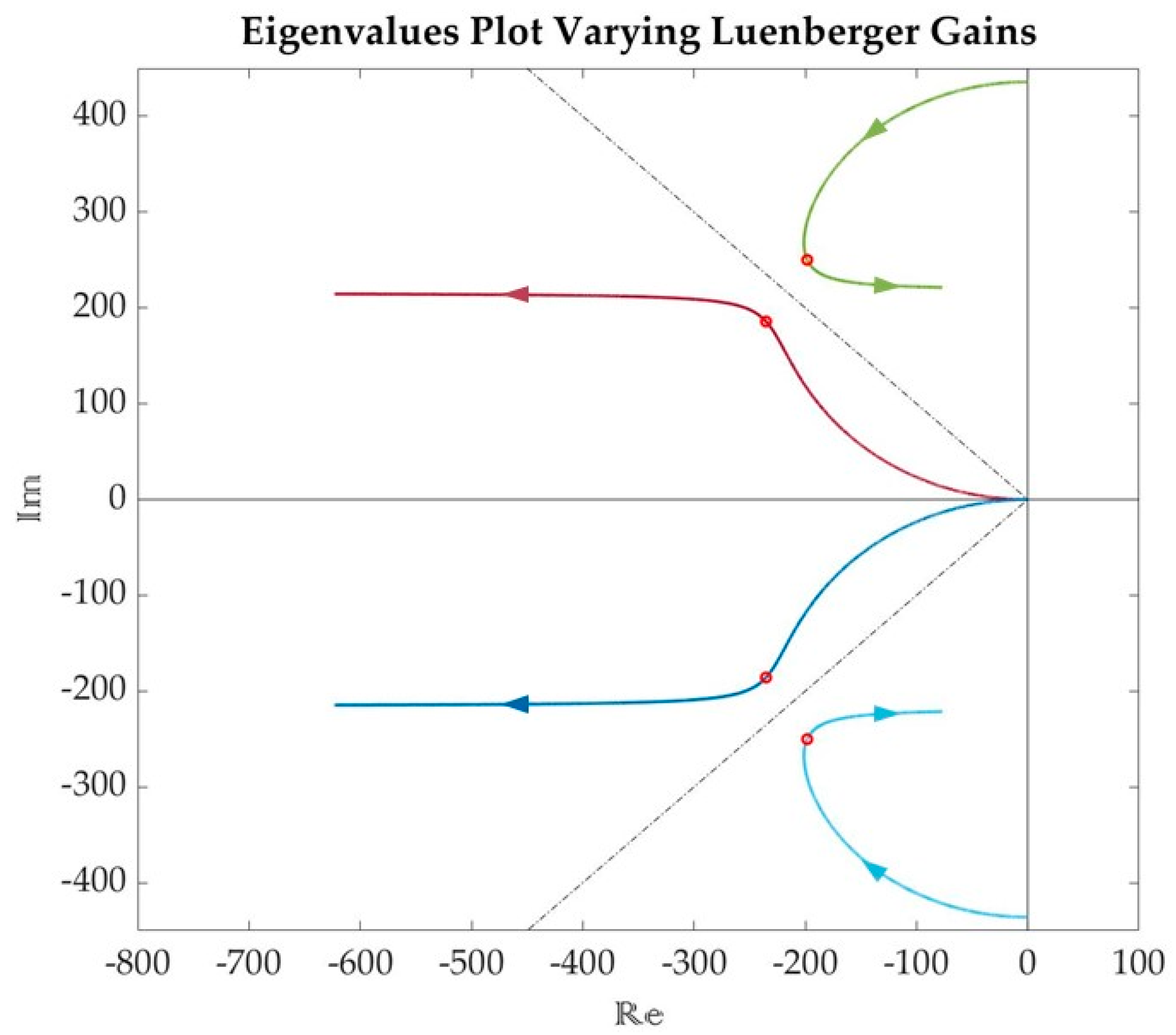
Through these parameters, it is possible to obtain the following graph, where the eigenvalues are represented varying the Luenberger gains and imposing the rated speed.

In this case, the following assumption in Equation (17) is considered:

$$K_r=-K_s$$

(17)

The condition in Equation (17) speeds up the algorithm and leads to good results in terms of system stability. In Figure 3, a plot of the eigenvalues varying Luenberger gains with the previous relationship is shown. The plot is obtained varying $K_s$ from −10 to 10 and, consequently, $K_r$ for 10 to −10.

Each color represents an eigenvalue that moves in the real–imaginary plane. Only eigenvalues on the left of the imaginary axis are represented. This shape is more or less constant for all the motors studied. Dashed axes represent the position of eigenvalues for which the system response has only one overshoot. The algorithm studied finds the Luenberger gains for which the eigenvalues are closest to the dashed axes. 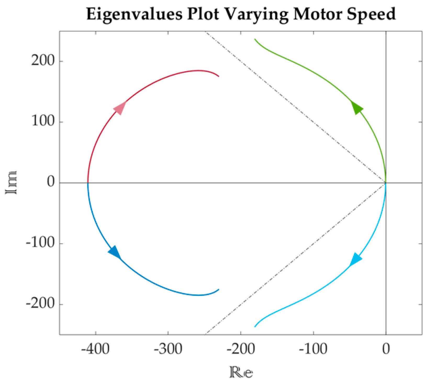Four eigenvalues resulting from gains $K_s=6.086$ and $K_r=-6.086$ are highlighted by a red circle. From this analysis, one derives that these two gains lead the system to stability and guarantee the best dynamic performance; there are other gains that lead to stability, but they do not guarantee the same dynamic properties. Furthermore, stability of these gains must be studied by varying the motor speed. In Figure 4 the latter analysis is shown.

When the speed is zero, the matrix becomes not invertible, so it is not possible to calculate the eigenvalues, but for every speed value greater than zero the eigenvalues exhibit a negative real part value. The last thing to do is to verify the behavior of the system in the simulations.

6. Filter and Cable Modeling and Compensation

In order to study the compensation strategy for the filter and cable, the entire system was implemented in the MATLAB/Simulink environment and is shown in Figure 5.

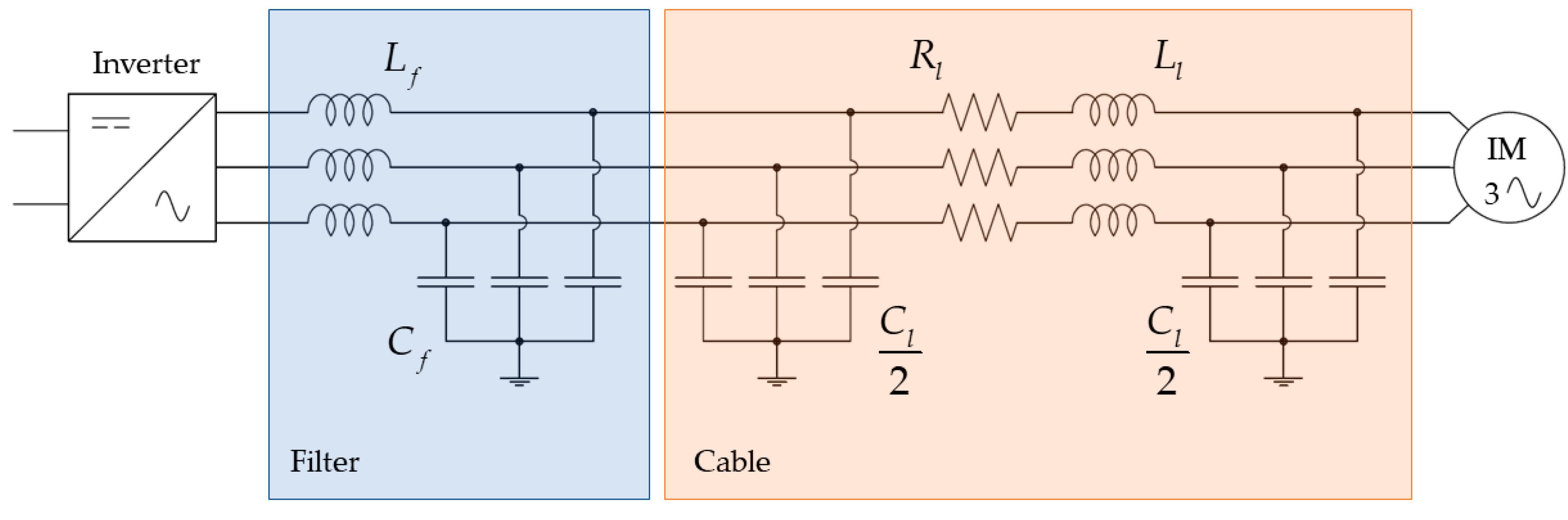
An eleven-level cascaded H-bridge inverter was used in this application. The model of this converter is shown in [10]. An LC filter was located downstream of the inverter, and it is shown in Figure 6, filter parameters were chosen in order to limit the amplitude of the harmonics injected into the cable [11].

The model for the cable was the π model, as shown in Figure 7. It is a third-order system, and it approximates the cable behavior.

As it will be shown below, the choice of this simplified model was enough to obtain a good compensation. The behavior of this model is compared with other models in [12]. The last component was the squirrel-cage induction motor; its model has been well defined in the previous sections.

The Luenberger observer needs the input variable of the machine and the output that are, respectively, the stator voltage and the stator currents. It is clear that these measures are not available because the motor is under the sea. The accessible measures are written below:

•

inverter voltages;

•

inverter currents;

•

output filter voltages; and

•

output filter currents.

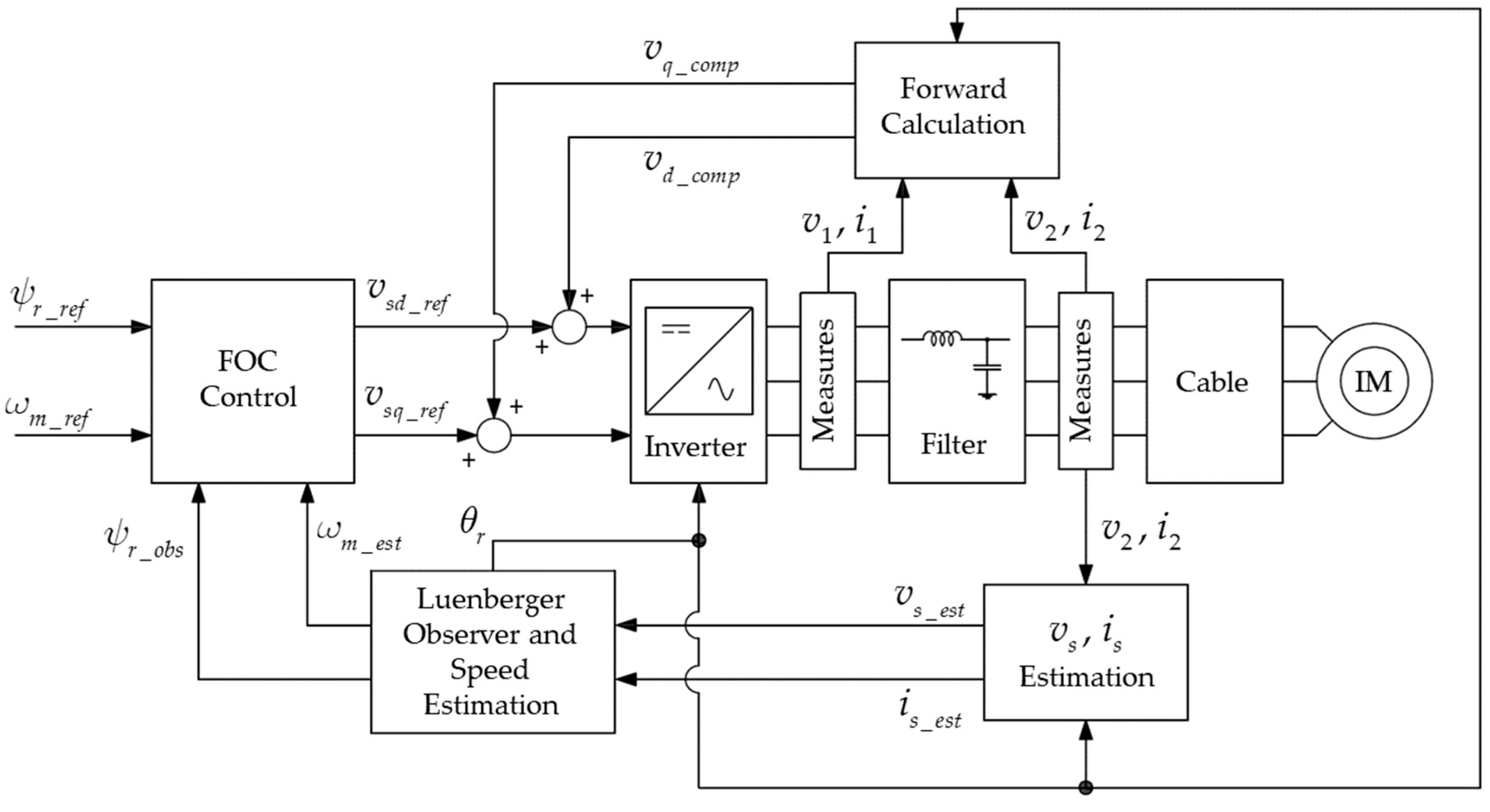
The inverter voltages are available only as inverter modulation signals. Starting from these values it is possible to estimate the stator voltage and the stator current, and also to estimate the voltage drop of the filter and cable, which will be added to the voltage references provided by the DFOC control, similar to that shown in [13] but using Park transformation. As shown in Section 3, the DFOC control returns as reference the values of stator voltage to be imposed on the motor through the inverter, so it is necessary to know the voltage drop to give the correct voltage to the motor. A block diagram of the improved SCDFOC algorithm is shown below in Figure 8.

First, the estimation of the stator voltage and currents will be shown; from the latter, it will be possible to obtain the coefficients to be added to the FOC references.

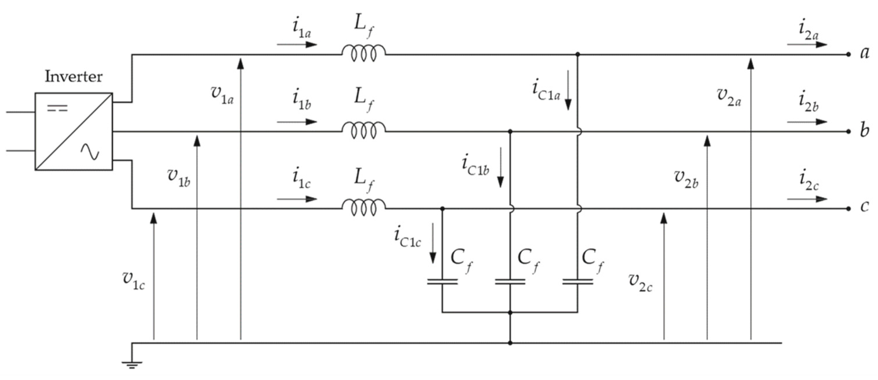
In Figure 7 and Figure 8, all the system variables are shown. Variables can be written as vectors as shown in Equations (18)–(20).

$${\mathbf{v}}_1=\left[\begin{array}{l}{v}_{1a}\\ v_{1b}\\ v_{1c}\end{array}\right];\hspace{0.17em}\hspace{0.17em}\hspace{0.17em}\hspace{0.17em}{\mathbf{i}}_1=\left[\begin{array}{l}{i}_{1a}\\ i_{1b}\\ i_{1c}\end{array}\right];\hspace{0.17em}\hspace{0.17em}\hspace{0.17em}\hspace{0.17em}{\mathbf{i}}_{C1}=\left[\begin{array}{l}{i}_{C1a}\\ i_{C1b}\\ i_{C1c}\end{array}\right];\hspace{0.17em}\hspace{0.17em}\hspace{0.17em}\hspace{0.17em}{\mathbf{v}}_2=\left[\begin{array}{l}{v}_{2a}\\ v_{2b}\\ v_{2c}\end{array}\right];$$

(18)

$${\mathbf{i}}_2=\left[\begin{array}{l}{i}_{2a}\\ i_{2b}\\ i_{2c}\end{array}\right];\hspace{0.17em}\hspace{0.17em}\hspace{0.17em}\hspace{0.17em}{\mathbf{i}}_{C2}=\left[\begin{array}{l}{i}_{C2a}\\ i_{C2b}\\ i_{C2c}\end{array}\right];\hspace{0.17em}\hspace{0.17em}\hspace{0.17em}\hspace{0.17em}{\mathbf{i}}_3=\left[\begin{array}{l}{i}_{3a}\\ i_{3b}\\ i_{3c}\end{array}\right];\hspace{0.17em}\hspace{0.17em}\hspace{0.17em}\hspace{0.17em}{\mathbf{i}}_{C3}=\left[\begin{array}{l}{i}_{C3a}\\ i_{C3b}\\ i_{C3c}\end{array}\right];$$

(19)

$${\mathbf{v}}_s=\left[\begin{array}{l}{v}_{sa}\\ v_{sb}\\ v_{sc}\end{array}\right];\hspace{0.17em}\hspace{0.17em}\hspace{0.17em}\hspace{0.17em}{\mathbf{i}}_s=\left[\begin{array}{l}{i}_{sa}\\ i_{sb}\\ i_{sc}\end{array}\right];$$

(20)

The variables, whose measurement is available, are as follows:

•

$i_1$: inverter currents;

•

$v_2$: filter output voltages; and

•

$i_2$: filter output currents.

Starting from these measures it is possible to estimate the motor voltages using Kirchhoff low as stated in Equation (21):

$${\mathbf{v}}_s={\mathbf{v}}_2-R_l\hspace{0.17em}{\mathbf{i}}_3-L_l\frac{d\hspace{0.17em}{\mathbf{i}}_3}{dt}$$

(21)

where:

$${\mathbf{i}}_3={\mathbf{i}}_2-{\mathbf{i}}_{C2}$$

(22)

$${\mathbf{i}}_{C2}=\frac{C_l}{2}\frac{d\hspace{0.17em}{v}_2}{dt}$$

(23)

So, it is possible to rewrite Equation (21) as shown in Equation (24):

$${\mathbf{v}}_s={\mathbf{v}}_2-R_l\left({\mathbf{i}}_2-\frac{C_l}{2}\frac{d\hspace{0.17em}{\mathbf{v}}_2}{dt}\right)-L_l\left(\frac{d\hspace{0.17em}{\mathbf{i}}_2}{dt}-\frac{C_l}{2}\frac{d^2{\mathbf{v}}_2}{d{t}^2}\right)$$

(24)

In addition, it is possible to estimate the motor currents as in Equation (25):

$${\mathbf{i}}_s={\mathbf{i}}_2-{\mathbf{i}}_{C2}-{\mathbf{i}}_{C3}$$

(25)

where:

$${\mathbf{i}}_{C3}=\frac{C_l}{2}\frac{d\hspace{0.17em}{\mathbf{v}}_s}{dt}$$

(26)

Then is possible to rewrite Equation (25) as in Equation (27)

$${\mathbf{i}}_s={\mathbf{i}}_2-\frac{C_l}{2}\left(\frac{d\hspace{0.17em}{\mathbf{v}}_2}{dt}+\frac{d\hspace{0.17em}{\mathbf{v}}_s}{dt}\right)$$

(27)

Note that in Equation (26) the voltage ${\mathbf{v}}_s$ is already an estimation.

From Equations (21) and (24), it is already possible to estimate the stator voltage and the stator current, but the equation components are mostly derivative components. It is well known that the derivative is critical for noise-affected signals, such as current or voltage measurements.

In order to avoid the use of derivative components, the Park transformation is adopted for the estimation. The angle used for the transformation is the angle provided by the Luenberger observer. The Park matrix is reported in (28).

$$k=k\left({\theta }_r\right)=\frac{2}{3}\left[\begin{array}{ccc}\sin \left({\theta }_r\right)& \sin \left({\theta }_r-\frac{2\pi }{3}\right)& \sin \left({\theta }_r+\frac{2\pi }{3}\right)\\ \cos \left({\theta }_r\right)& \cos \left({\theta }_r-\frac{2\pi }{3}\right)& \cos \left({\theta }_r+\frac{2\pi }{3}\right)\\ \frac{1}{2}& \frac{1}{2}& \frac{1}{2}\end{array}\right]$$

(28)

Assuming that:

$${\mathbf{v}}_s=k^{-1}\left({\theta }_r\right){\mathbf{v}}_{sdq}$$

(29)

where:

$${\mathbf{v}}_{sdq}=\left[\begin{array}{c}{v}_{sd}\\ v_{sq}\\ 0\end{array}\right]$$

(30)

Equation (24) is transformed as in Equation (31):

$$k^{-1}{\mathbf{v}}_{sdq}=k^{-1}{\mathbf{v}}_{2dq}-R_l\hspace{0.17em}{k}^{-1}{\mathbf{i}}_{2dq}+R_l\frac{C_l}{2}\frac{d}{dt}\left(k^{-1}{\mathbf{v}}_{2dq}\right)-L_l\frac{d}{dt}\left(k^{-1}{\mathbf{i}}_{2dq}\right)-L_l\frac{C_l}{2}\frac{d^2}{d{t}^2}\left(k^{-1}{\mathbf{v}}_{2dq}\right)$$

(31)

Multiplying (31) for matrix $k$, one obtains Equation (32)

$${\mathbf{v}}_{sdq}={\mathbf{v}}_{2dq}-R_l\hspace{0.17em}{\mathbf{i}}_{2dq}+R_l\frac{C_l}{2}k\frac{d}{dt}\left(k^{-1}{\mathbf{v}}_{2dq}\right)-L_l\hspace{0.17em}k\frac{d}{dt}\left(k^{-1}{\mathbf{i}}_{2dq}\right)-L_l\frac{C_l}{2}k\frac{d^2}{d{t}^2}\left(k^{-1}{\mathbf{v}}_{2dq}\right)$$

(32)

Remembering that $k$ is a function of ${\theta }_r$ as reported in Equation (28), Equation (33) can be demonstrated, where the product between the transformation matrix and the derivative is developed and simplified.

$$k\left({\theta }_r\right)\frac{d}{dt}\left(k^{-1}\left({\theta }_r\right){\mathbf{v}}_{2dq}\right)=\frac{d\hspace{0.17em}{\theta }_r}{dt}{\mathbf{S} \mathbf{v}}_{2dq}+\frac{d}{dt}{\mathbf{v}}_{2dq}$$

(33)

where:

$$\mathbf{S}=\left(\begin{array}{ccc}0& -1& 0\\ 1& 0& 0\\ 0& 0& 0\end{array}\right)$$

(34)

and:

$$\frac{d\hspace{0.17em}{\theta }_r}{dt}={\omega }_r=\frac{{\omega }_{est}}{c_p}$$

(35)

So, Equation (33) became:

$$k\left({\theta }_r\right)\frac{d}{dt}\left(k^{-1}\left({\theta }_r\right){\mathbf{v}}_{2dq}\right)={\omega }_r{\mathbf{S} \mathbf{v}}_{2dq}+\frac{d}{dt}{\mathbf{v}}_{2dq}$$

(36)

In addition, for the second order derivative, the relations can be derived from Equation (33) as in Equation (37).

$$k\left({\theta }_r\right)\frac{d^2}{d{t}^2}\left(k^{-1}\left({\theta }_r\right){\mathbf{v}}_{2dq}\right)=-{\omega }_r^2\hspace{0.17em}{\mathbf{v}}_{2dq}+\frac{d^2}{d{t}^2}{\mathbf{v}}_{2dq}$$

(37)

So, (32) can be rewritten as Equation (38).

$${\mathbf{v}}_{sdq}={\mathbf{v}}_{2dq}-R_l\hspace{0.17em}{\mathbf{i}}_{2dq}+R_l\frac{C_l}{2}\left({\omega }_r\mathbf{S}\hspace{0.17em}{\mathbf{v}}_{2dq}+\frac{d}{dt}{\mathbf{v}}_{2dq}\right)-L_l\hspace{0.17em}\left({\omega }_r\mathbf{S}\hspace{0.17em}{\mathbf{i}}_{2dq}+\frac{d}{dt}{\mathbf{i}}_{2dq}\right)-L_l\frac{C_l}{2}\left({\omega }_r^2{\mathbf{v}}_{2dq}+\frac{d^2}{d{t}^2}{\mathbf{v}}_{2dq}\right)$$

(38)

It has been empirically demonstrated through simulations that in Equation (38), the derivative components are neglectable, so the relation can be rewritten as in Equation (39)

$${\mathbf{v}}_{sdq}={\mathbf{v}}_{2dq}-R_l\hspace{0.17em}{\mathbf{i}}_{2dq}+R_l\frac{C_l}{2}{\omega }_r\mathbf{S}\hspace{0.17em}{\mathbf{v}}_{2dq}-L_l\hspace{0.17em}{\omega }_r\mathbf{S}\hspace{0.17em}{\mathbf{i}}_{2dq}-{\omega }_r^2{L}_l\frac{C_l}{2}{\mathbf{v}}_{2dq}$$

(39)

Dividing (39) in its components, two relations are obtained, as shown in Equations (40) and (41).

$$v_{sd}=v_{2d}-R_l\hspace{0.17em}{i}_{2d}-R_l\frac{C_l}{2}{\omega }_r{\mathbf{v}}_{2q}-L_l\hspace{0.17em}{\omega }_r\hspace{0.17em}{i}_{2q}-{\omega }_r^2{L}_l\frac{C_l}{2}{v}_{2d}$$

(40)

$$v_{sq}=v_{2q}-R_l\hspace{0.17em}{i}_{2q}+R_l\frac{C_l}{2}{\omega }_r{\mathbf{v}}_{2d}-L_l\hspace{0.17em}{\omega }_r\hspace{0.17em}{i}_{2d}-{\omega }_r^2{L}_l\frac{C_l}{2}{v}_{2q}$$

(41)

The same procedure can be applied to the stator current. Starting from Equation (27), it is possible to obtain Equation (42):

$${\mathbf{i}}_{sdq}={\mathbf{i}}_{2dq}-\frac{C_l}{2}\left({\omega }_r\mathbf{S}\hspace{0.17em}{\mathbf{v}}_{2dq}+\frac{d}{dt}{\mathbf{v}}_{2dq}+{\omega }_r\mathbf{S}\hspace{0.17em}{\mathbf{v}}_{sdq}+\frac{d}{dt}{\mathbf{v}}_{sdq}\right)$$

(42)

Moreover, here, derivative components are neglectable.

$${\mathbf{i}}_{sdq}={\mathbf{i}}_{2dq}-\frac{C_l}{2}{\omega }_r\mathbf{S}\hspace{0.17em}{\mathbf{v}}_{2dq}-\frac{C_l}{2}{\omega }_r\mathbf{S}\hspace{0.17em}{\mathbf{v}}_{sdq}$$

(43)

where:

$$i_{sd}=i_{2d}+\frac{C_l}{2}{\omega }_r{v}_{2q}+\frac{C_l}{2}{\omega }_r{v}_{sq}$$

(44)

$$i_{sq}=i_{2q}-\frac{C_l}{2}{\omega }_r{v}_{2d}-\frac{C_l}{2}{\omega }_r{v}_{sd}$$

(45)

The obtained vectors ${\mathbf{v}}_{sdq}$ and ${\mathbf{i}}_{sdq}$ must be transformed from Park’s reference system to Clarke’s in order to use them in the Luenberger Observer. As shown, the advantage of using the Park Transformation lies in the decomposition of the derivative. The same considerations can be made for the voltage drops compensations. The voltage that the inverter must impose on the system in order to reach the voltage reference of the machine clamps is shown in Equation (46).

$${\mathbf{v}}_{1\_ref}={\mathbf{v}}_{s\_ref}+L_f\frac{d}{dt}{\mathbf{i}}_1+R_l\hspace{0.17em}{\mathbf{i}}_3+L_l\frac{d}{dt}{\mathbf{i}}_3$$

(46)

Substituting in (46) only the available quantities, one obtains Equation (47).

$${\mathbf{v}}_{1\_ref}={\mathbf{v}}_{s\_ref}+L_f\frac{d}{dt}{\mathbf{i}}_1+R_l\hspace{0.17em}{\mathbf{i}}_2-R_l\frac{C_l}{2}\frac{d}{dt}{\mathbf{v}}_2+L_l\frac{d}{dt}{\mathbf{i}}_2-L_l\frac{C_l}{2}\frac{d^2}{d{t}^2}{\mathbf{v}}_2$$

(47)

These equations can be elaborated as the previous ones, obtaining Equation (48)

$${\mathbf{v}}_{1dq\_ref}={\mathbf{v}}_{sdq\_ref}+L_f\hspace{0.17em}{\omega }_r\mathbf{S}\hspace{0.17em}{\mathbf{i}}_{1dq}+R_l\hspace{0.17em}{\mathbf{i}}_{2dq}-R_l\frac{C_l}{2}{\omega }_r\mathbf{S}\hspace{0.17em}{\mathbf{v}}_{2dq}+L_l\hspace{0.17em}{\omega }_r{\mathbf{S} \mathbf{i}}_{2dq}+{\omega }_r^2{L}_l\frac{C_l}{2}{\mathbf{v}}_{2dq}$$

(48)

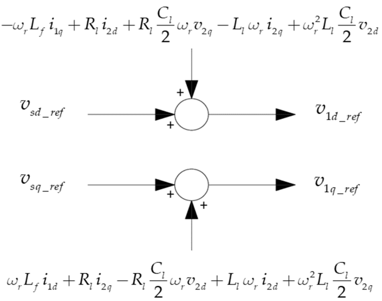
Equation (48) can be written in its components, as shown in Equations (49) and (50).

$$v_{1d\_ref}=v_{sd\_ref}-{\omega }_r{L}_f\hspace{0.17em}{i}_{1q}+R_l\hspace{0.17em}{i}_{2d}+R_l\frac{C_l}{2}{\omega }_r{v}_{2q}-L_l\hspace{0.17em}{\omega }_r\hspace{0.17em}{i}_{2q}+{\omega }_r^2{L}_l\frac{C_l}{2}{v}_{2d}$$

(49)

$$v_{1q\_ref}=v_{sq\_ref}+{\omega }_r{L}_f\hspace{0.17em}{i}_{1d}+R_l\hspace{0.17em}{i}_{2q}-R_l\frac{C_l}{2}{\omega }_r{v}_{2d}+L_l\hspace{0.17em}{\omega }_r\hspace{0.17em}{i}_{2d}+{\omega }_r^2{L}_l\frac{C_l}{2}{v}_{2q}$$

(50)

It is necessary to add the calculated voltage drops, as shown in Figure 9, to adequately compensate for the line and the filter. This compensation works properly when the line parameters are the rated ones, but, as already mentioned, the line undergoes temperature variations, which means parameters variations; so, it is important to investigate through the simulations if the parameter variations affect significantly the drive behavior.

7. Simulation Results

The entire system is implemented in MATLAB/Simulink environment.

The simulator is divided into two parts: the control, which is a discrete-time region (the entire control has been designed to have a frequency of 3.3 kHz), and the model of the physical elements.

Table 2. Filter and Line parameters.

	Parameter	Value
$L_f$	Filter inductance	5.3 mH
$C_f$	Filter capacitance	2.1 µF
$L$	Cable length	19.74 km
$R_l$	Cable resistance	0.0787 Ω/km
$L_l$	Cable inductance	0.3384 mH/km
$C_l$	Cable capacitance	0.385 µF/km

contains the filter and line parameters, respectively.

The line is modeled using a three-phase distributed parameters block provided by Simscape, which is based on the Bergeron’s travelling wave method, described in [14]. This method should generally be chosen when the system length is enough to allow the propagation of waves through the entire length of the line. In a first phase of the study, the inverter was not introduced in the simulator; this was in order to evaluate the performance of the algorithm in the absence of the harmonics generated by the switching devices. This was also to obtain a faster simulator that ensured that the calculated Luenberger gains were right. After that phase, the multilevel inverter (11 level cascade H-bridge) was introduced.

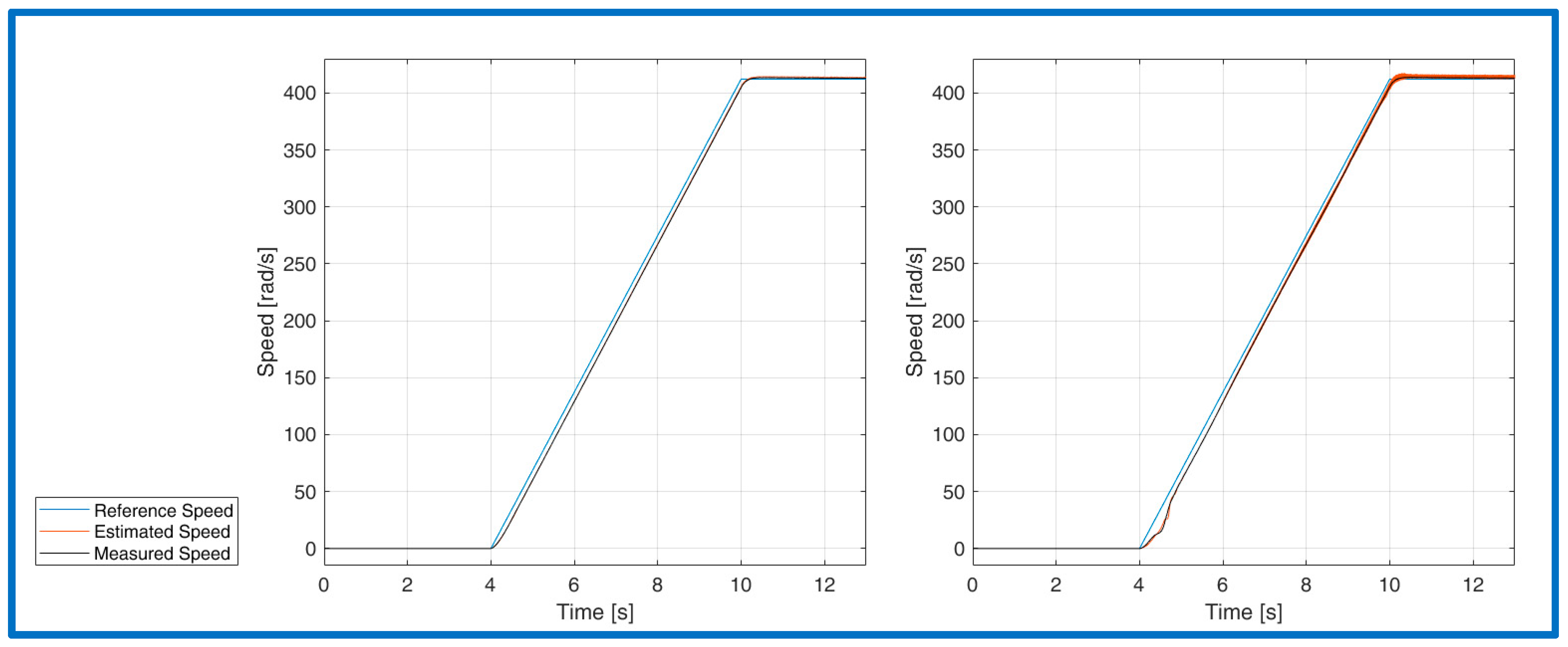
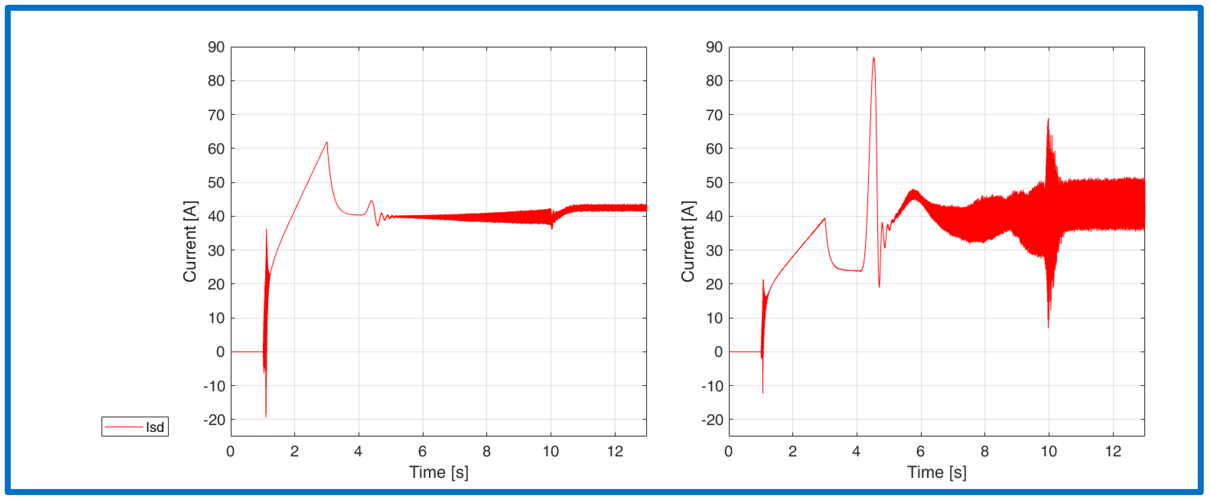
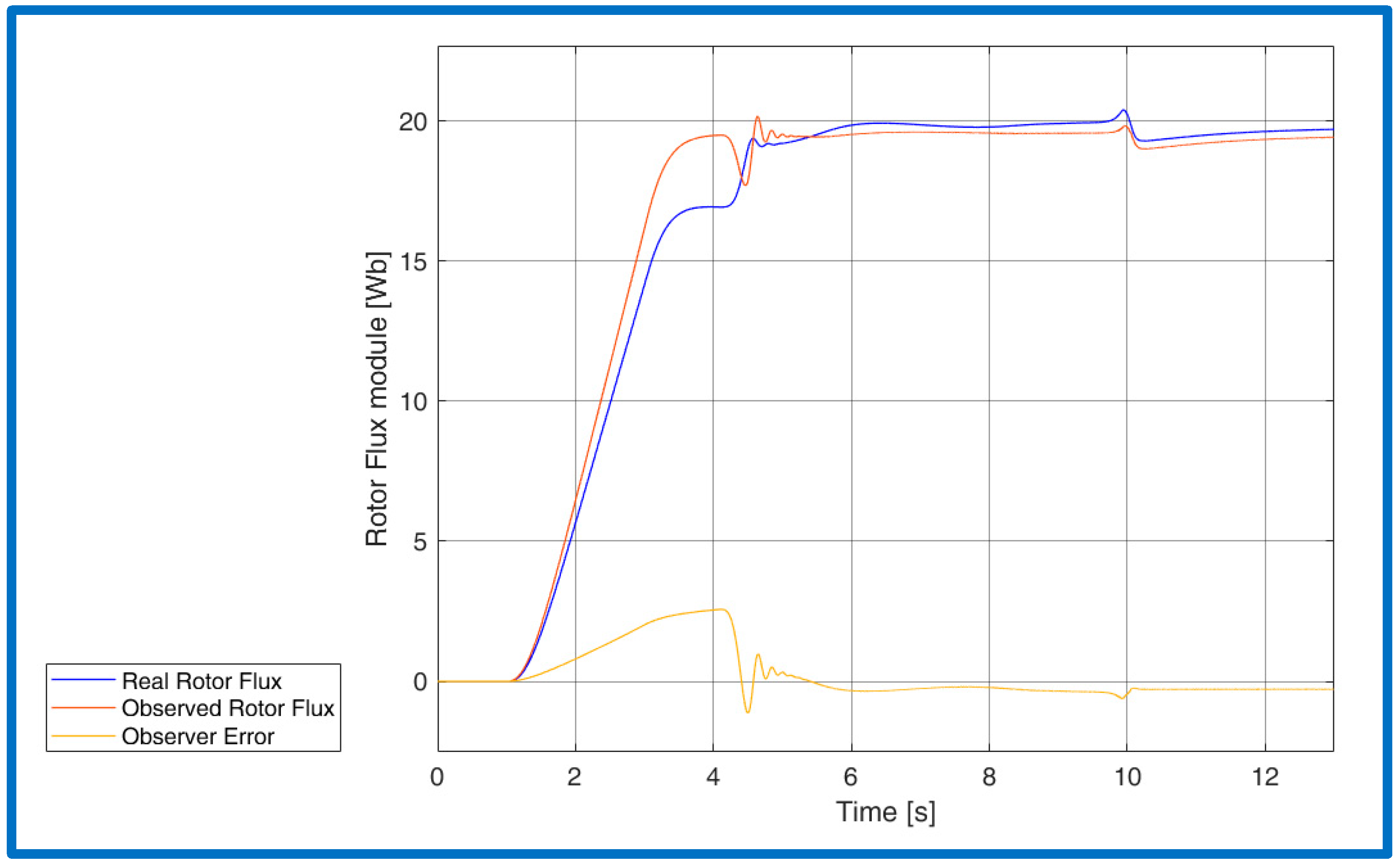
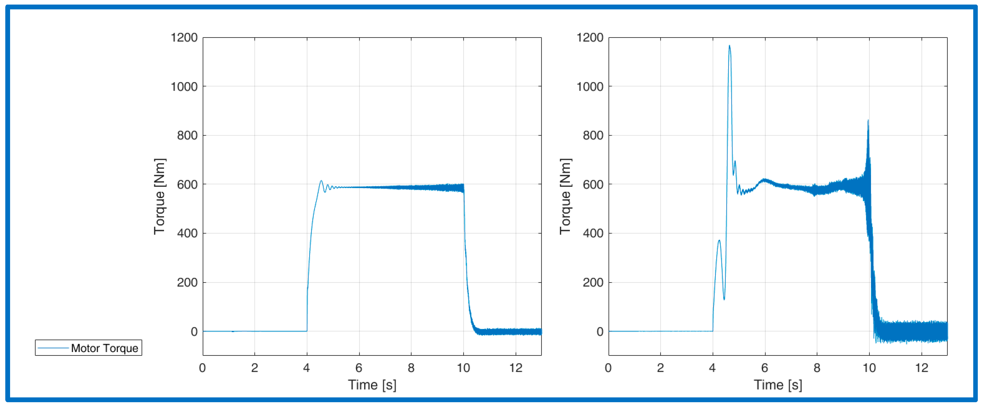
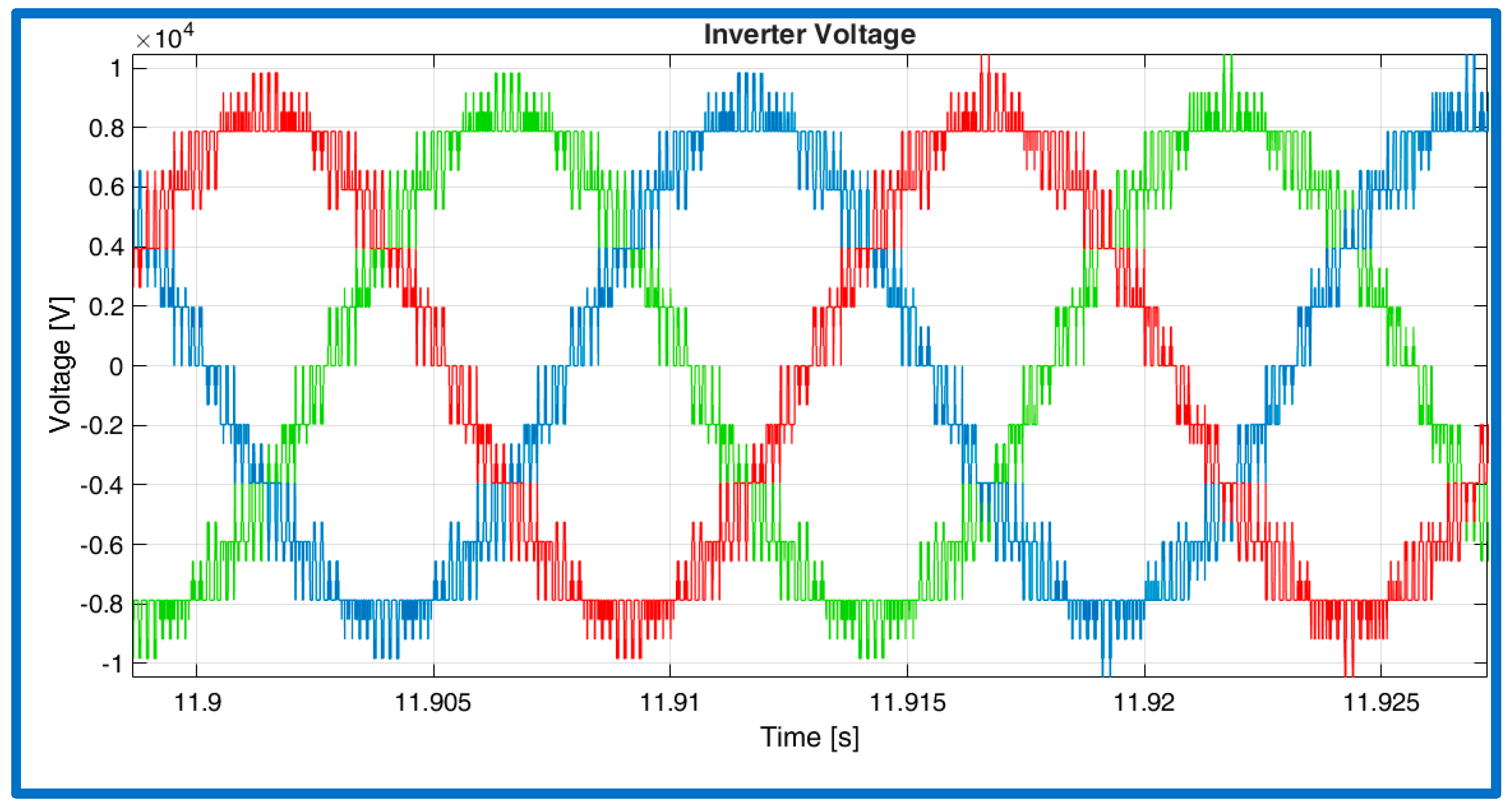
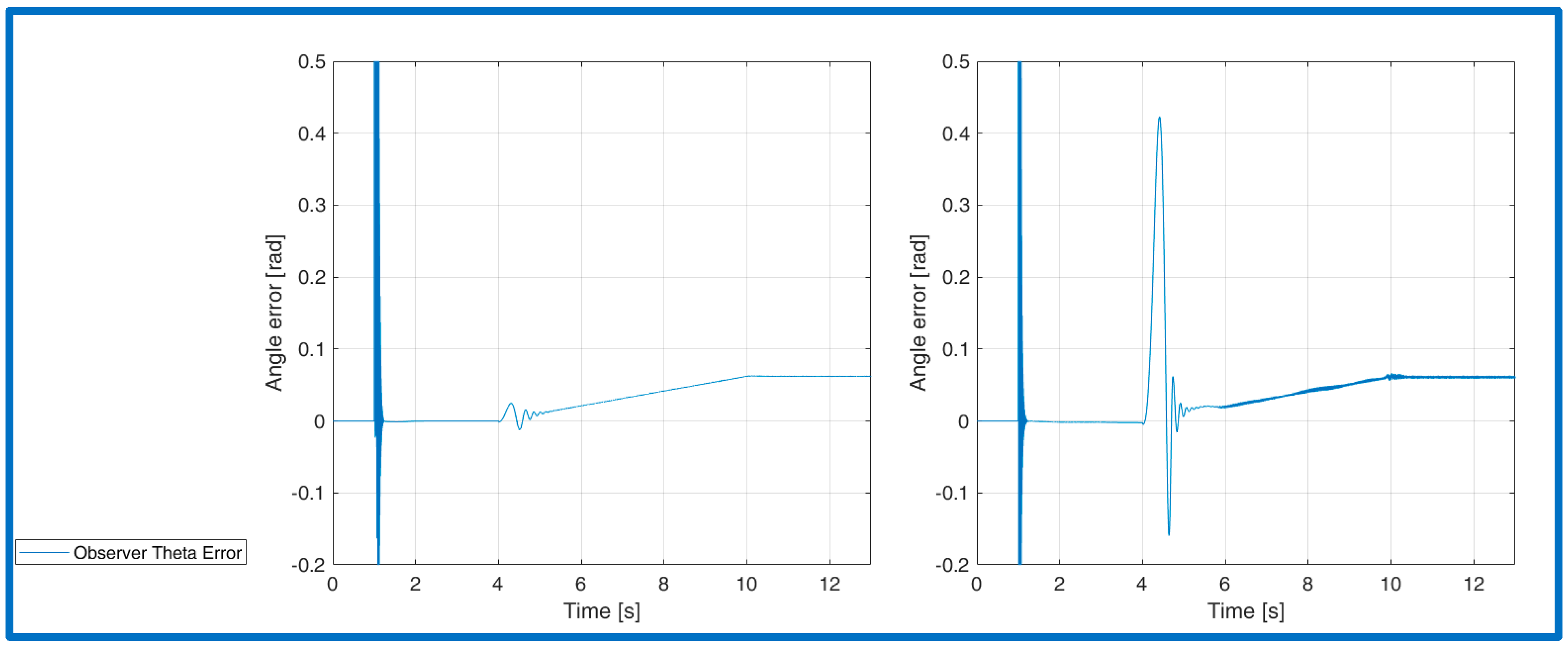
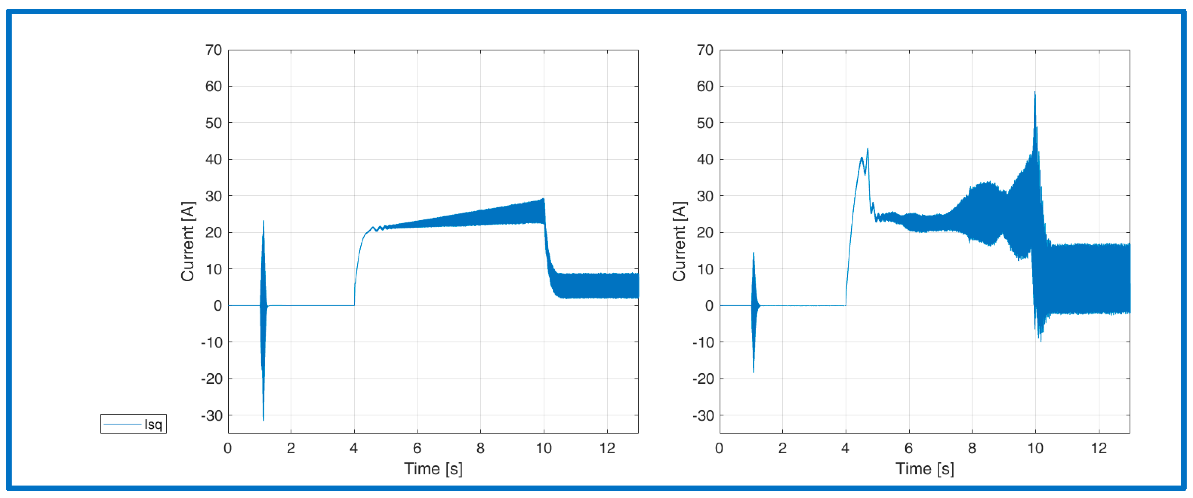
In the following graphics, the comparison of the no-load starting of the system powered with ideal voltage generators and with the inverter voltage is proposed. In Figure 10 the comparison between observed and real rotor flux is presented, in Figure 11 estimated and measured speed are shown, Figure 12 shows the motor torque, in Figure 13 the observer rotor flux angle error is shown, Figure 14 and Figure 15 display d-q-axis stator currents and Figure 16 shows the inverter voltages.

It is possible to note how, introducing the inverter voltage the error between the observed module of the flux and real one increased, as in Figure 10, especially in the flux-up phase. Furthermore, the error between the observed angle and the real one was affected by some oscillations (Figure 13). These errors are caused primarily by two factors: the introduction of the harmonics generated by the inverter voltages and the approximation made using the π model of the long cable in the equation to estimate the stator voltage. Furthermore, it should be also noted that the derivative components were neglected in both the compensation and the estimation algorithms. Despite the presence of these errors, the system works properly as one can note from the motor speed, machine torque and currents profile in Figure 11, Figure 12, Figure 14 and Figure 15, respectively.

In order to demonstrate the influence of the π model approximation, the same simulation test was realized implementing the π model for the cable, instead of the previous continuous model, and the comparison between the observed and real rotor flux module graph is showed in Figure 17. Note that in both cases the cable was compensated for with a π model; however, in Figure 10 the cable was simulated with the continuous model, whereas in Figure 17, it was simulated in with the π model.

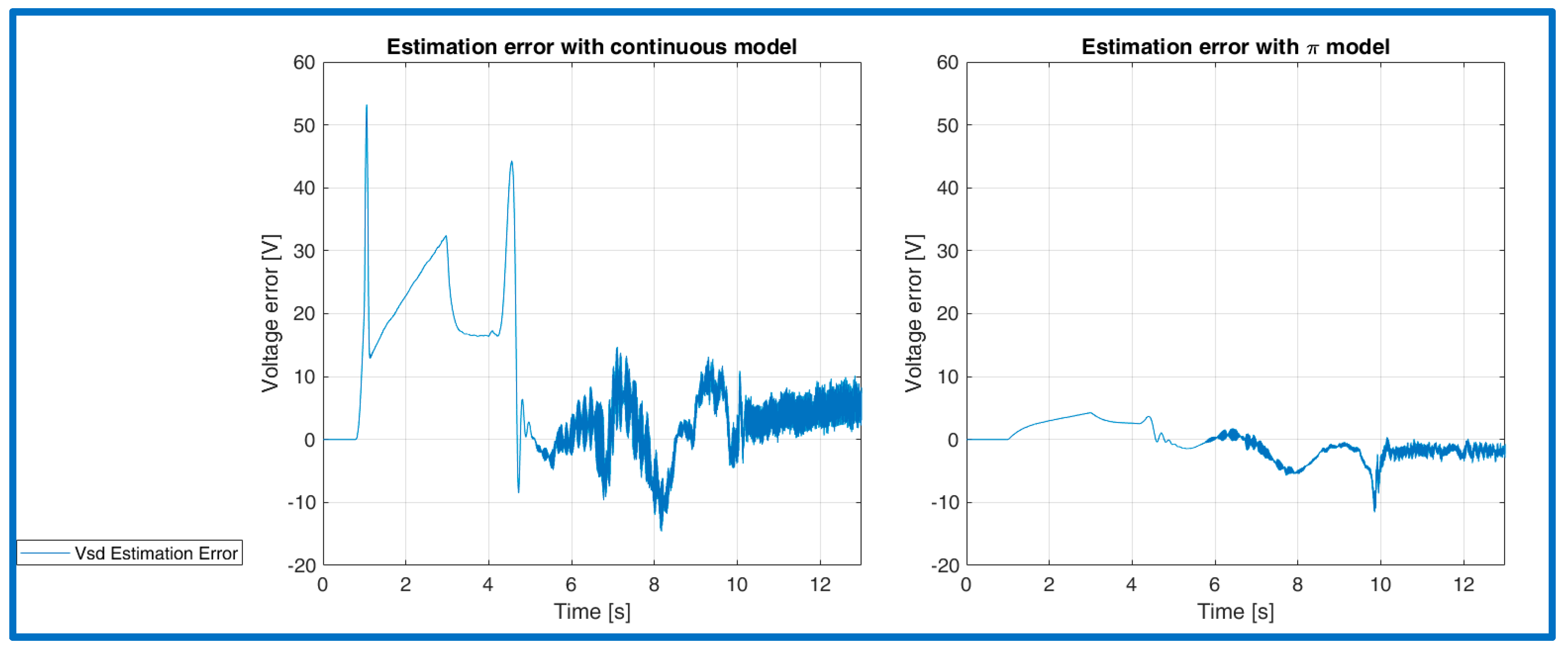
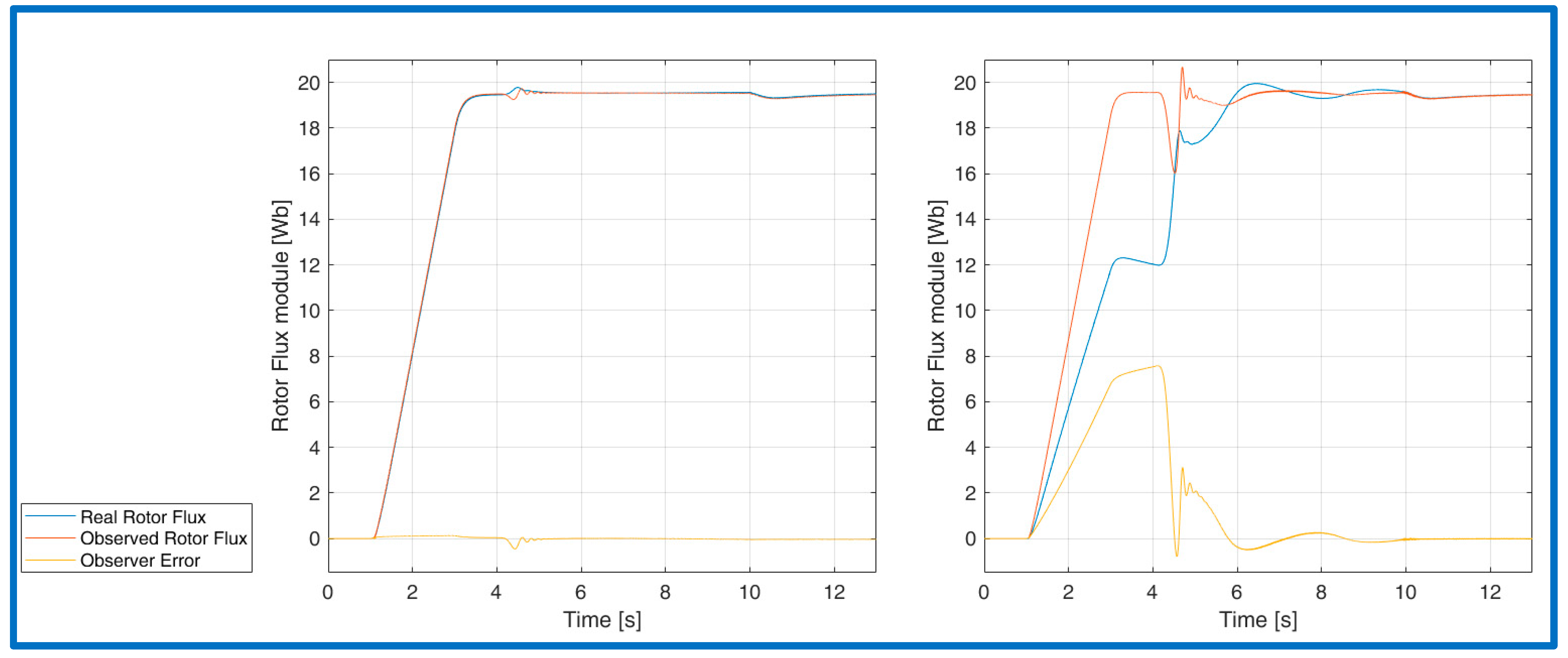
As already explained, this difference depends on the approximation used to estimate the stator voltage; in particular, it depends on the error on the d-axis of the estimation. In Figure 18, the error between the measured stator voltage and the estimated one is shown in two cases, on the left using the continuous model to simulate the cable and on the right using the π model.

It is evident that the observer error depends on this estimation error; in the case of ideal sinusoidal voltages the error is near to zero, especially using the PI model to simulate the cable, and this is the reason why the observer error is low in that case. The estimation error becomes higher during the acceleration of the machine, and it reaches a constant low value that can vary with torque applications and speed variation. From the previous simulations, it is evident that the absence of derivatives components could affect the system operation but not significantly. In order to study the system stability, another simulation was proposed using the continuous model for the line and the inverter model. In this simulation after the no-load start, two torque steps were applied, and during the second one a speed variation was applied. The first step was equal to $0.8\cdot T_n$, and it started at the second 15 and had a duration of 5 s, after which the load torque returned to zero. The second step started at the second 23, its amplitude was $0.6\cdot T_n$, and it lasted until the end of the simulation, which had a total duration of 30 s.

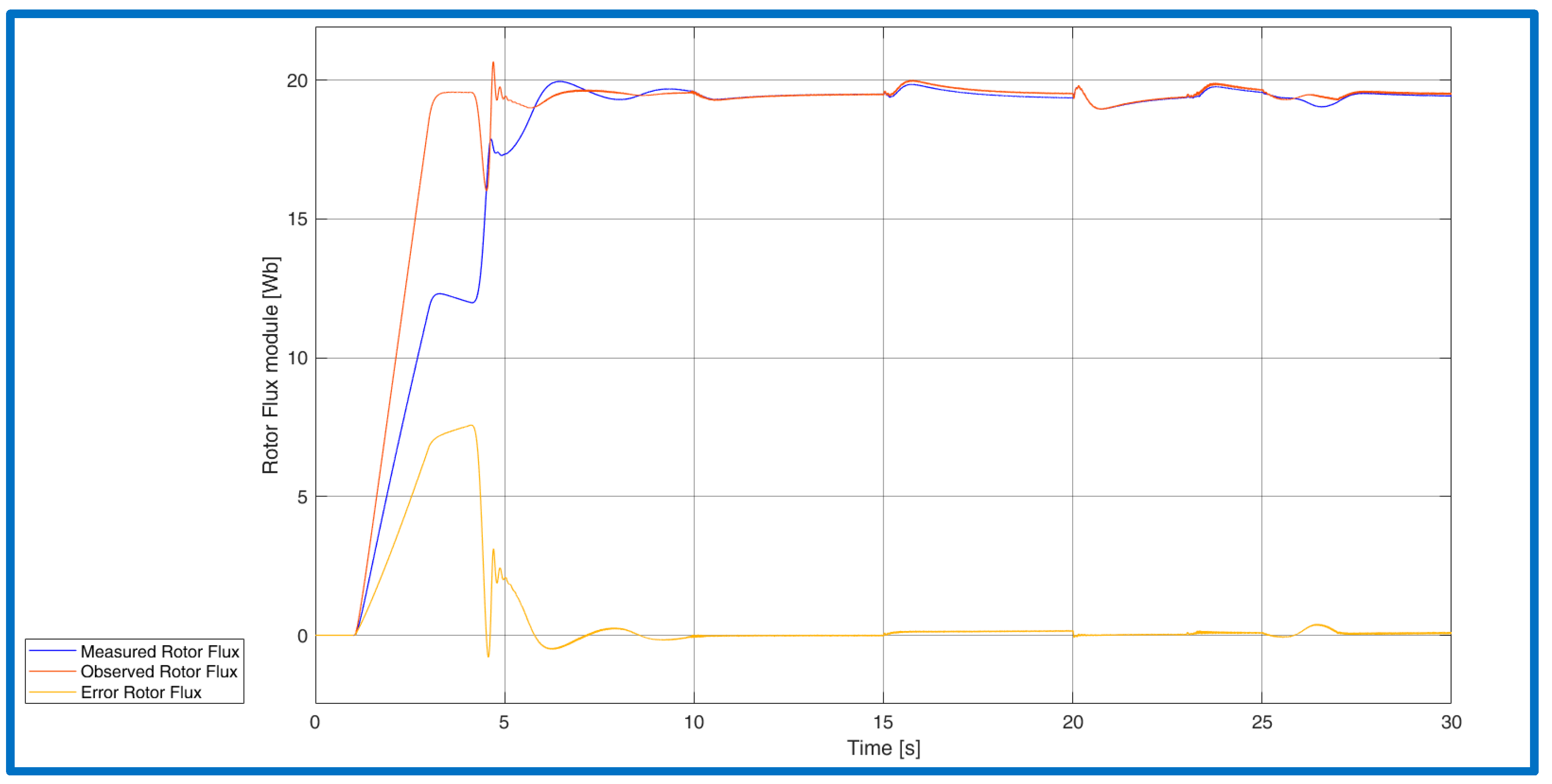
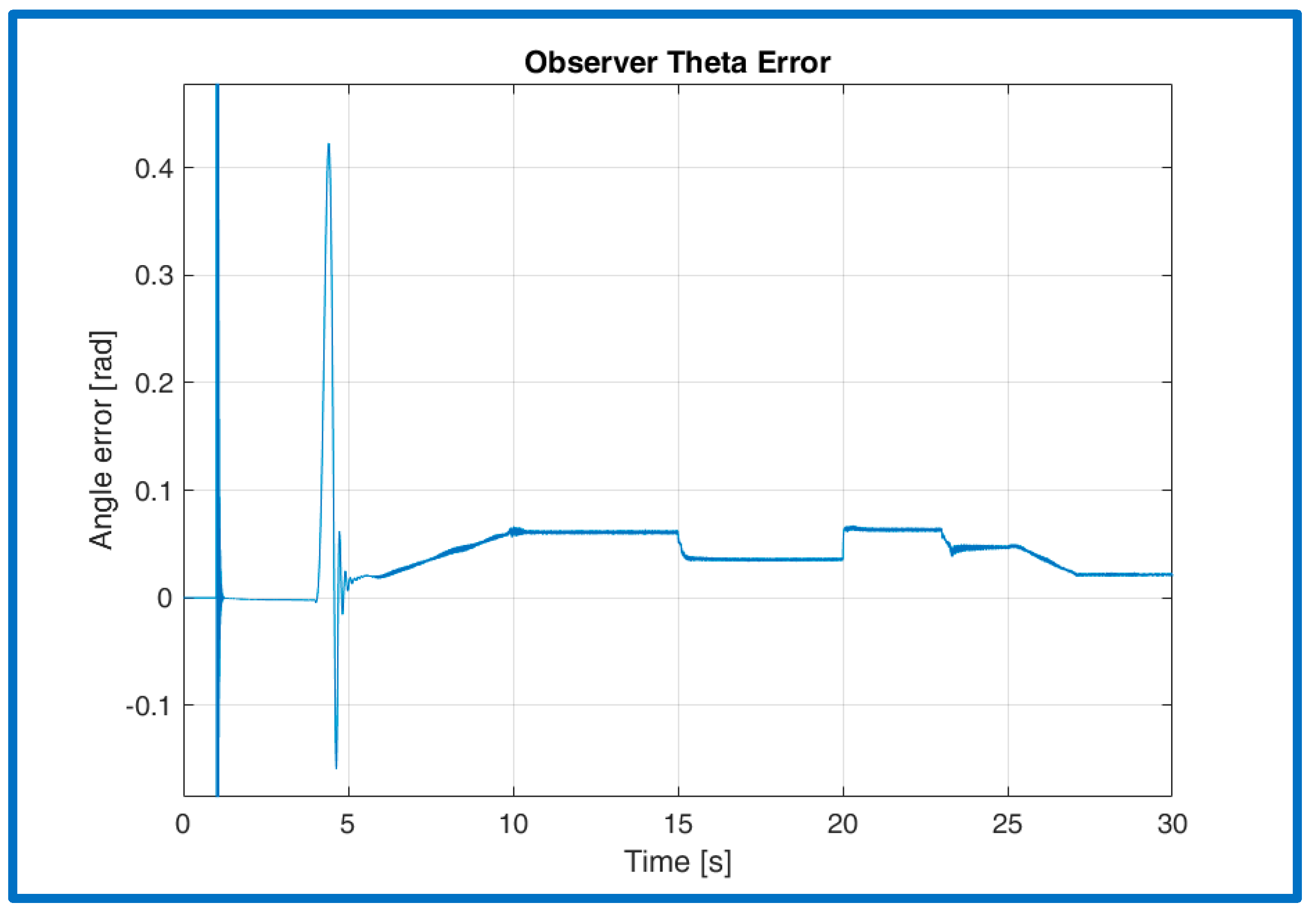
In Figure 19 and Figure 20, the rotor flux module and the rotor flux angle error are shown, respectively. It is possible to note that when the step torque was applied, the measured rotor torque module varied, and the observed one followed it with a neglectable error. Moreover, the angle reduced its error during the step torque, thanks to the higher current that led to a more precise stator voltage estimation.

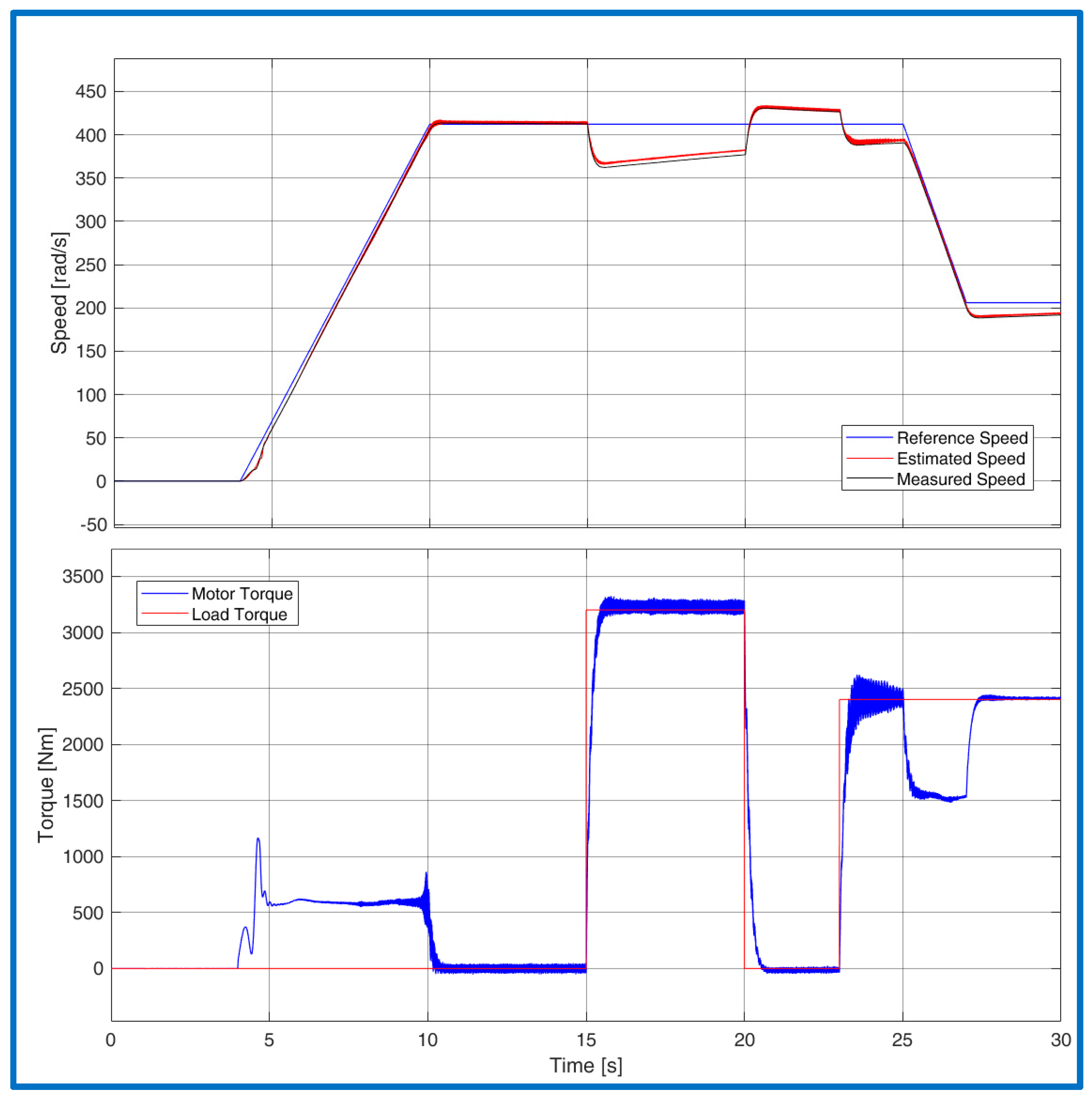
In Figure 21, the mechanical variables are reported. Analyzing the first plot, which shows the comparison between the estimated speed, the real one, and the reference, it is evident that the machine had a speed loss during the torque steps; however, the regulation intervened to bring the speed back to the reference value. This phenomenon is observable in the graph between seconds 15 and 20, when the step torque was applied.

The presence of the cable made it necessary to reduce the speed of the regulators to avoid resonances; consequently, the dynamics of some quantities such as torque, shown in Figure 21, become slower. However, this is not an issue in the considered application.

8. Conclusions

In this paper, a compensated direct field-oriented sensorless control for an induction motor with filter and long cable was presented. A Luenberger observer was used to obtain the rotor flux module and angle starting from the stator voltages and currents. The stability of the Luenberger observer was studied, and an algorithm for the optimal selection of the Luenberger gains was developed.

The filter and the line were placed between the inverter and the motor, and starting from the system equations, a stator voltage and current estimation were developed to provide these machine variables to the Luenberger observer. Moreover, from the same equations, a feed-forward technique was adopted in order to compensate for the voltages drops of the filter and of the cable and in order to supply the motor with the output of the FOC algorithm.

The entire system was implanted in the MATLAB/Simulink environment, and simulation tests were carried out to evaluate the CDFOC performances in sensorless mode.

The results obtained from the simulations can be compared with those obtained in article [13], where a different compensation calculation method and different control algorithms were proposed. Comparing the two no load starts, it is possible to see that the SCDFOC dynamics looks a little faster, but this may depend on the speed controllers gains. The main difference is that the simulations in this article were made using a long cable model, in particular a continuous model of the cable that is closer to reality; instead in the article cited above, a PI model was used. Furthermore, the length of the cables was different, in this article the cable studied was 19.74 km long, while in the above mentioned publication the cable was 1 km long. So, the results are not easily comparable.

The algorithms presented for estimation and compensation can be used also with other types of induction machine control, such as Direct Torque Control [15] and V/Hz control [16] to compensate for the cable effects. The major limitation of the compensation algorithm that resulted from this preliminary study was mainly due to the oscillations generated by the system composed by cable, filter, and motor and how the control algorithm of induction machines was affected by them. In the future, laboratory tests will be carried out; in particular, high power machines and components will be used in order to validate what has been proposed in this article and to provide experimental results very close to the application reality.