District Heating of Buildings by Renewable Energy Using Thermochemical Heat Transmission

Abstract

The decarbonisation of building heating in urban areas can be achieved by heat pumps connected to district heating networks. These could be ‘third-generation’ (85/75 °C), ‘fourth-generation’ (50/40 or 50/25 °C) or ‘fifth-generation’ (near ambient) water loops. Networks using thermochemical reactions should require smaller pipe diameters than water systems and be more economic. This work investigates thermochemical transmission systems based on liquid–gas absorption intended for application in urban district heating networks where the main heat source might be a MW scale heat pump. Previous studies of absorption for heat transmission have concentrated on long distance (e.g., 50 km) transmission of heat or cold utilizing waste heat from power stations or similar but these are not directly applicable to our application which has not been investigated before. Absorbent-refrigerant pairs are modelled using water, methanol and acetone as absorbates. Thermodynamic properties are obtained from the literature and modelling carried out using thermodynamic analysis very similar to that employed for absorption heat pumps or chillers. The pairs with the best performance (efficiency and power density) both for ambient loop (fifth-generation) and high temperature (fourth-generation) networks use water pairs. The next best pairs use methanol as a refrigerant. Methanol has the advantage of being usable at ambient temperatures below 0 °C. Of the water-based pairs, water–NaOH is good for ambient temperature loops, reducing pipe size by 75%. Specifically, in an ambient loop, heat losses are typically less than 5% and the heat transferred per volume of pumped fluid can be 30 times that of a pumped water network with 10 K temperature change. For high temperature networks the heat losses can reach 30% and the power density is 4 times that of water. The limitation with water–NaOH is the low evaporating temperature when ambient air is the heat source. Other water pairs perform better but use lithium compounds which are prohibitively expensive. For high temperature networks, a few water- and methanol-based pairs may be used, but their performance is lower and may be unattractive.

1. Introduction

It is commonly suggested that the decarbonisation of building heating in urban areas is best achieved by large, efficient, and adaptable heat pumps connected to district heating networks. Conventionally these would be ‘third-generation’ (85/75 °C), ‘fourth-generation’ (50/40 or 50/25 °C) or ‘fifth-generation’ (near ambient) water loops [1]. In urban environments the costs of retrofitting a district heating network are very high and the installation can be very disruptive. Both the cost and level of disruption increase rapidly with the pipe diameter used. The networks using thermochemical (TC) reactions should require far smaller pipe diameters than pumped water systems, and be far less costly to install and, correspondingly, more economical.

This paper seeks to evaluate possible sorption TC reactions that might be used in this way. This section surveys some of the previous work in this area, explains the TC system and components, and suggests suitable figures of merit to characterize and compare them. Section 2 presents the different absorption pairs that are considered, and Section 3 describes the mathematical approach to modelling the performance, presenting the equations used for all the components: desorber, absorber, condenser, pump, evaporator and solution heat exchangers. The results are firmly grounded in sorption thermodynamics and use robust measured data on material pairs from the literature. Section 4 presents the results for ambient, fifth-generation loops, (Section 4.1) and for higher temperature fourth-generation loops (Section 4.2). Within these sections different absorption pairs using a number of refrigerants (water, methanol and acetone) are compared and contrasted. Finally, Section 5 presents the discussion and conclusions. Appendix A and Appendix B contain the thermochemical data used, enabling replication or further exploration of our results. A methodical thermodynamic study based on a practical district heating application/requirement and comparing so many absorption pairs is a new contribution to the topic.

Previously, there have been studies using both open and closed thermochemical systems to transfer heat. Closed systems have included the possibility of using the decomposition/composition of methanol [2] or metal hydride reactions [3,4]. However, the temperatures in the methanol reaction are not applicable in district heating and the exotic metal alloys employed in hydride reactions are prohibitively expensive. Kang et al. [5] proposed a ‘solution transportation absorption’ (STA) similar to that analysed in this paper but intended for district cooling powered by waste heat from remote power stations. Both lithium bromide–water and ammonia–water absorption pairs were analysed. Wang [6] suggested the absorption of ammonia refrigerant into water absorbent as a means of transferring heat over long distances. However, in our application of district heating, safety considerations preclude the use of large quantities of pressurized ammonia solution.

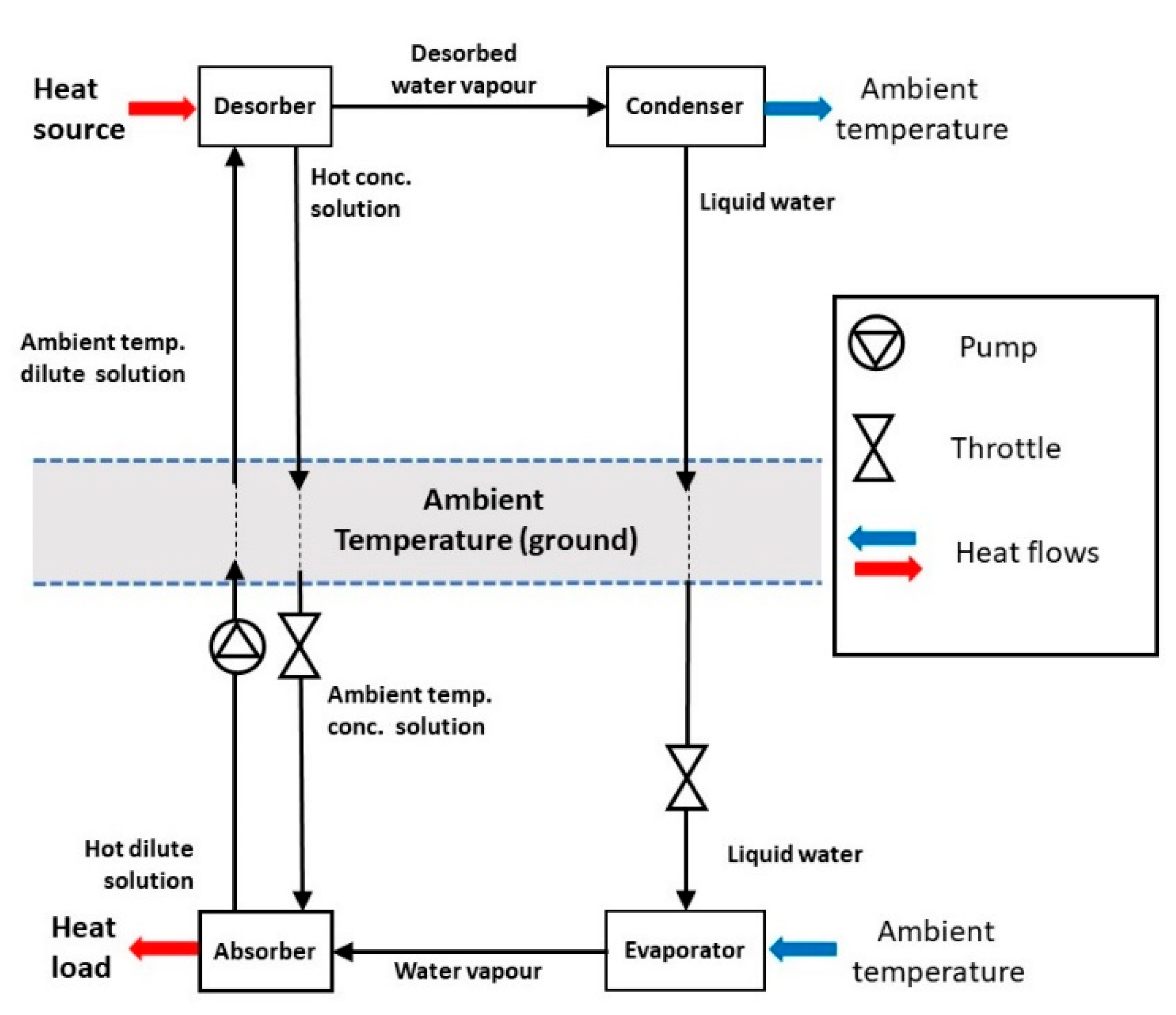
Open systems utilize concentrated and dilute solutions of liquid desiccants such as LiBr in which water absorption (either for humidity control or the heating effect) occurs at the point of use. Geyer et al. [7,8] develops ideas for waste heat utilization and storage in addition to transport but the concept is particularly useful when integrated with drying or humidification needs as part of the demand. Our focus is purely on heat transportation within a district heating system and the performance of possible absorption pairs. A closed system using water, acetone or an alcohol as a low-pressure refrigerant that is absorbed or desorbed into a hydroxide, bromide or similar salt is proposed. The simplest such arrangement to transport heat would be as shown in Figure 1.

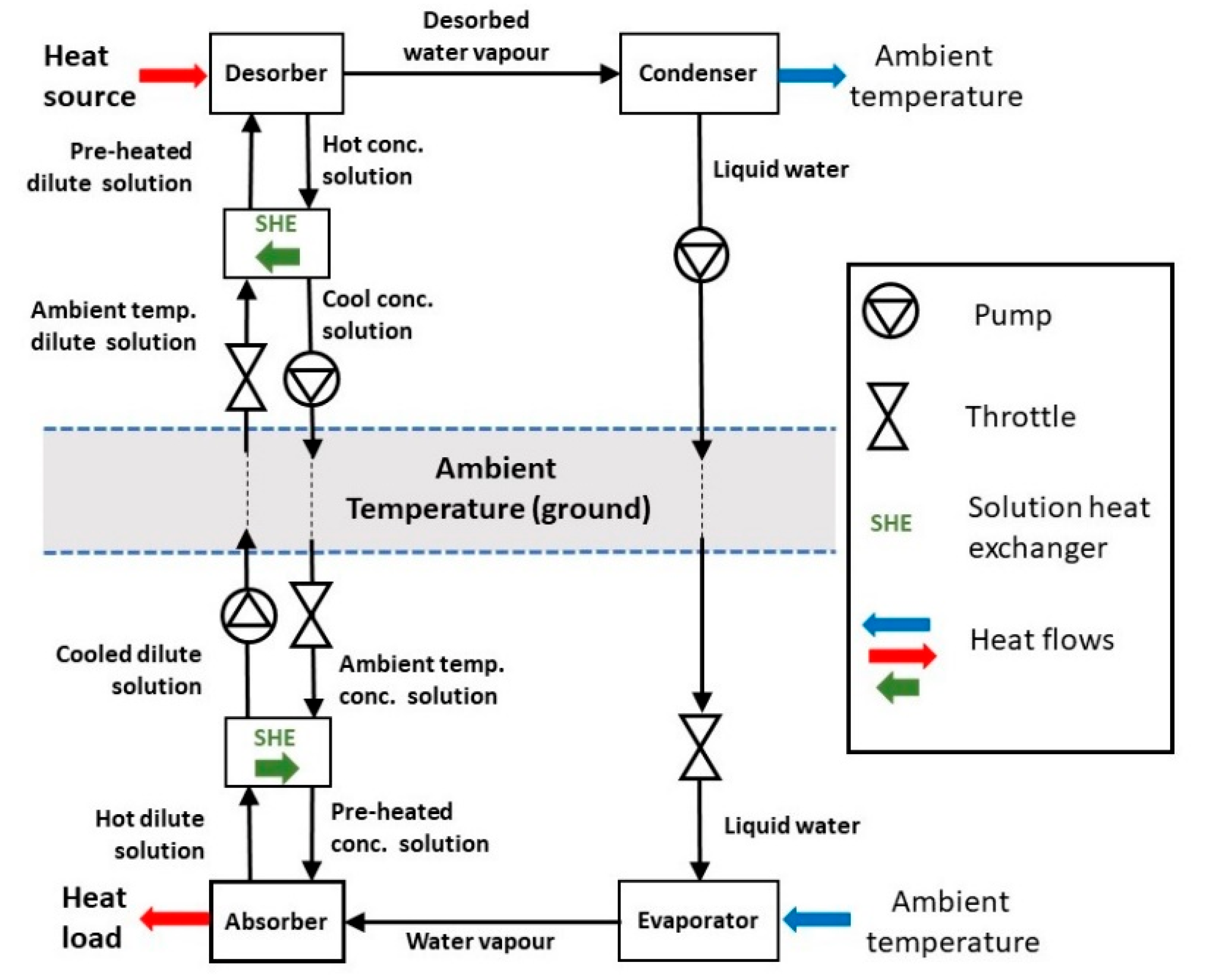
Heat for distribution, typically from a heat pump or industrial waste heat, is used to desorb water from the dilute solution. The water vapour is condensed at as low a temperature as possible to maximise the concentration change. The liquid water and concentrated solution can then be pumped to the delivery location. At the delivery point the liquid water can be evaporated by ambient temperature heat and be absorbed into the concentrated solution, releasing the heat of absorption to the load. The concentrated solution is then pumped back to the heat source side of the system. Because the heat of absorption is, in general, large compared to the sensible heat of the solutions above ambient, the basic system would be feasible, but not as efficient as it could be. Even with very high levels of pipe insulation the three liquid lines would lose significant amounts of sensible heat as they are pumped over long distances. This loss can be reduced by at least 80% by the use of solution heat exchangers (SHEs), as shown in Figure 2.

On the source side, the SHE preheats the incoming dilute ambient temperature solution (the worst case is that it is at ambient temperature) with the outgoing hot concentrated solution. Thus, the hot solution enters the network only a little above ambient, minimizing the sensible heat loss. On the delivery side the SHE performs a similar role, preheating the incoming concentrated solution with the hot exiting dilute solution. The other practical difference between the basic and proposed systems is that the pumped liquids would be at atmospheric pressure or a little higher and throttled down to absorption/desorption pressure at point of use. Pumping at a sub-atmospheric pressure would both be impractical and encourage air ingress that would reduce the system efficiency.

In this paper, the possible use of a number of absorption pairs that might be suitable for district heating TC networks is investigated. Most use water as the refrigerant as in Figure 1 and Figure 2 above, but a few use methanol or acetone. At low ambient temperatures (below about 5 °C) it becomes impracticable to boil water in the evaporator since the pressure is very low and the water may freeze. It is possible to boil water out of an anti-freeze solution or a very dilute solution of the sorbate, but it would be better to avoid the complexity. If a ground source can be used, the evaporating temperature can be kept high enough to avoid problems but using the air as an ambient heat source needs another approach. One possibility is to use methanol or acetone as the refrigerant rather than water. They both can be used down to −10 °C or less but they have lower latent and absorption heats than water. This results in less energy being transmitted per unit volume pumped around the network. One other possibility that would allow the use of water would be to boost the temperature level of the ambient by 5 or 10 K using a vapour compression heat pump. At such a small temperature lift, it is feasible to do this with a COP > 9 and so it may be a technically viable approach. However, in this study a number of water, acetone and methanol absorption pairs are simply characterised.

There are two characteristics that define the performance of a pair under set conditions of ambient temperature, desorption temperature and absorption temperature. These are the efficiency, simply the heat delivered divided by the heat from the source, and a measure of the heat transferred per unit volume of fluid that must be pumped through the network. Since the objective is to achieve lower diameter and hence lower pipework installation costs than with a conventional water network, a physically meaningful comparison has been chosen. The energy transferred by the volume flowing in the three pipe TC system is calculated and then the temperature differential that would be necessary to transfer the same energy using the sensible heat in a conventional two pipe (flow and return) water system is obtained. This is referred to as ΔT H₂O. Thus, if the calculated value were only 10 K the total flow would be the same as a conventional water system with a 10 K difference between flow and return (as is typical). If however ΔT H₂O were 100 K, it implies that the total volume being pumped was roughly 1/10 of that needed by a conventional district heating system. Should a TC system be compared with a water system having a higher flow–return temperature difference of say 20 K then ΔT H₂O would have to exceed 20 K for there to be any advantage

In the methodology section below, the thermodynamic calculations are described. They require full mixture property data obtained from sources in the literature. The results plot ΔT H₂O v. the efficiency for combinations of ambient temperature (strictly the evaporating and condensing temperature), absorption temperature (heat delivery) and desorption temperature (heat supply). The results are used to suggest which pairs may be of interest and worthy of further investigation in future, more detailed, studies.

2. Materials

The absorbate is a refrigerant that must be capable of boiling at ambient temperature and ideally should have a high latent heat to ensure high energy transport per unit mass. Water is ideal apart from its low vapour pressure. The lowest practicable evaporating temperature is about 5 °C. Alcohols and acetone do not have such high latent heat but can be boiled at lower (sub-zero) temperatures which is advantageous in certain climatic conditions.

Different groups of substances such as salts, alkalis, acids, organic compounds and ionic liquids can be used as absorbents. In addition to their good thermodynamic properties when forming a solution, other criteria such as availability, price, recyclability, environmental compatibility, toxicity and chemical stability should be considered in their selection.

The absorbent pairs that have been modelled in this paper are:

• Water-based pairs: LiBr, LiCl, LiI, LiBr + LiI, LiBr + LiNO₃, LiCl + LiNO₃, LiBr + ZnCl₂ + CaBr₂, NaOH, Ca(NO₃)₂
• Methanol-based pairs: ZnBr₂, LiBr, LiI + ZnBr₂, LiBr + ZnBr₂, LiBr + ZnCl₂
• Acetone-based pair: ZnBr₂

A full list of the thermophysical properties of the refrigerants and of the correspondent absorbent pairs extracted from the literature can be found in Appendix A and Appendix B, respectively.

3. Methods

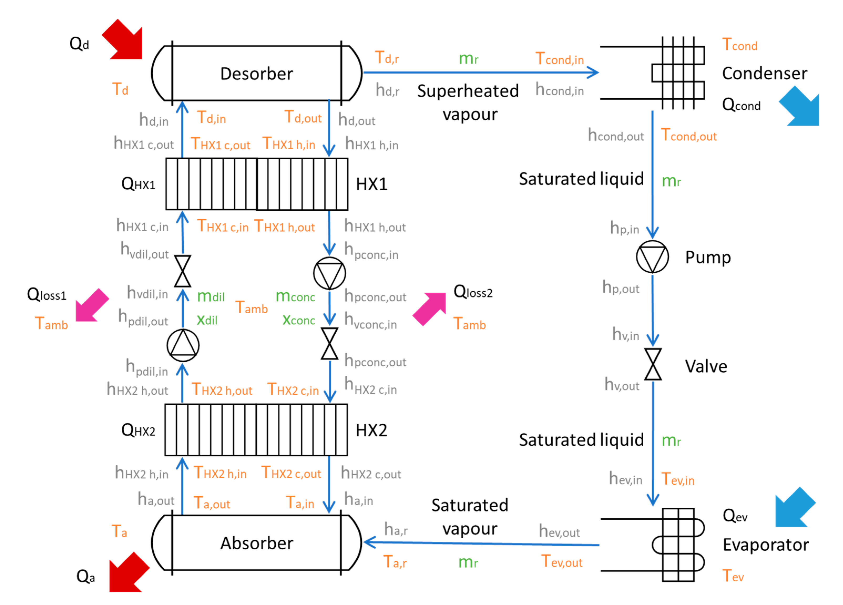
This section describes the approach developed to model and simulate the absorption cycle described in Figure 3.

The salt concentration in the solution that is circulated between the desorber and absorber and vice versa is represented by the symbol x and it is given as the mass percentage of the solution. It is defined as:

$$x=\raisebox{1ex}{$m_{salt}$}\!\left/ \!\raisebox{-1ex}{$m_{solution}$}\right.·100$$

(1)

where:

$$m_{solution}=m_{salt}+m_{abs}$$

(2)

$m_{salt}\mathrm{being}$the mass of salt and $m_{abs}$ the mass of absorbent.

The mass of the concentrated solution ($m_{conc}$, solution flowing between the desorber and the absorber) is equal to the sum of the mass of the salt $\left(m_{salt}\right)$ and the mass of the absorbent $\left(m_{abs}\right)$ (refrigerant that has not been desorbed in the desorbed and that gets pumped to and from the desorber/absorber).

$$m_{conc}=m_{salt}+m_{abs}$$

(3)

The mass of the dilute solution ($m_{dil}$, solution flowing between the absorber and desorber) is equal to the sum of the mass of the concentrated solution $\left(m_{conc}\right)$ and the mass of the desorbed refrigerant ($m_r$, refrigerant flowing through the condenser and evaporator).

$$m_{dil}=m_{conc}+m_r=m_{salt}+m_{abs}+m_r$$

(4)

In the simulation, attention must be paid to the maximum and minimum concentration limits of the solution modelled as reported in the Appendix A and Appendix B. Higher salt% in the solution can result in reaching the crystallization limit and could cause blockages in the system.

The concentrations of the dilute and concentrated solutions are defined as:

$$x_{conc}=\frac{m_{salt}}{m_{salt}+m_{abs}}·100$$

(5)

$$x_{dil}=\frac{m_{salt}}{m_{salt}+m_{abs}+m_r}·100$$

(6)

The mass of refrigerant flowing through the condenser and evaporator is the difference between the mass of the dilute $\left(x_{dil}\right)$and concentrated $\left(x_{conc}\right)$ solutions. For simplicity the calculations are all based on a value of $1 \mathrm{kg}/\mathrm{s}$.

$$m_r=m_{dil}-m_{conc}=1 \mathrm{kg}/\mathrm{s}$$

(7)

The concentration of the concentrated solution $\left(x_{conc}\right)$ is set by the temperature of the desorber $\left(T_d\right)$ and by the temperature of the condenser $\left(T_{cond}\right)$. On the other hand, the concentration of the dilute solution $\left(x_{dil}\right)$ is set by the temperature of the absorber $\left(T_a\right)$ and by the temperature of the evaporator $\left(T_{ev}\right)$. Both concentrations can be calculated with the Saturated Pressure equations corresponding to each salt/refrigerant pair included in Appendix A and Appendix B.

The masses of salt and absorbent in the solutions can be calculated from the dilute and concentrated concentrations with the following equations:

$$m_{salt}=-\frac{m_r}{\frac{100}{x_{conc}}-\frac{100}{x_{dil}}}$$

(8)

$$m_{abs}=\frac{m_r}{\frac{100}{x_{conc}}-\frac{100}{x_{dil}}}-\frac{100·m_r}{x_{conc}·\left(\frac{100}{x_{conc}}-\frac{100}{x_{dil}}\right)}$$

(9)

3.1. Desorber

The heat driving the desorption $\left(Q_d\right)$ is delivered to the desorber and solution at $T_d$. It is assumed that the temperature of the desorbed refrigerant ($T_{d,r}$, flowing towards the condenser) and the temperature of the concentrated solution ($T_{d,out}$, flowing towards the absorber) are both equal to the desorbing temperature $\left(T_d\right)$.

$$T_{d,r}=T_{d,out}=T_d$$

(10)

In addition, assuming there are no losses between desorber and condenser their pressures are equal:

$$p_d=p_{cond}$$

(11)

The refrigerant leaving the desorber is assumed to be in a superheated state since it will be at the desorber temperature but at a pressure lower than the saturation pressure for that temperature, which is the saturation pressure of the condenser at ambient temperature. Its enthalpy can be calculated by the corresponding equation for each refrigerant included in the Appendix A and Appendix B.

The energy balance of the desorber is calculated using the following equation:

$$Q_d=m_r{h}_{d,r}+m_{conc}{h}_{d,out}-m_{dil}{h}_{d,in}$$

(12)

where $Q_d$ is the heat input to the desorber, $m_{conc}$ is the mass of the concentrated solution, $m_{dil}$ is the mass of the dilute solution, $m_r$ is the mass of the refrigerant leaving the desorber, $h_{d,in}$ is the enthalpy of the dilute solution as it enters the desorber, $h_{d,out}$ is the enthalpy of the concentrated solution as it leaves the desorber and $h_{d,r}$ is the enthalpy of the superheated refrigerant as it leaves the desorber.

3.2. Absorber

The heat output of the absorbent $\left(Q_a\right)$ is delivered in the absorber and to the solution at $T_a$. It is assumed that the temperature of the dilute solution ($T_{a,out}$, flowing towards the desorber) is equal to the absorbing temperature $\left(T_a\right)$.

$$T_{a,out}=T_a$$

(13)

In addition, assuming there are no losses between absorber and evaporator their pressures are equal:

$$p_a=p_{ev}$$

(14)

In addition, it is assumed that there are no heat losses or gains to the refrigerant flowing from the evaporator to the absorber, therefore the enthalpy of the refrigerant entering the absorber is:

$$h_{a,r}=h_{ev,out}$$

(15)

The energy balance of the absorber is calculated using the following equation:

$$Q_a=m_r{h}_{a, r}+m_{conc}{h}_{a,in}-m_{dil}{h}_{a,out}$$

(16)

where $Q_a$ is the energy released in the absorber, $m_{dil}$ is the mass of the dilute solution, $m_{dil}$ is the mass of the concentrated solution, $m_r$ is the mass of the refrigerant entering the absorber, $h_{a,in}$ is the enthalpy of the concentrated solution entering the absorber, $h_{a,out}$ is the enthalpy of the dilute solution leaving the absorber and $h_{a,r}$ is the enthalpy of the saturated vapour refrigerant entering the absorber.

3.3. Condenser

In the system, both the condenser and the evaporator are assumed to be air-cooled and therefore dependent on both ambient conditions and on the effectiveness of the heat exchangers used. For the purpose of this simulation study, it is assumed that perfect heat exchangers are used between the ambient air and the condenser/evaporator resulting in their temperatures being equal. If required, a particular temperature difference can be assumed when interpreting the results.

$$T_{cond}=T_{ev}=T_{amb}$$

(17)

Assuming there are no heat losses between the desorber and condenser, the hot flow input temperature $\left(T_{cond,in}\right)$ corresponds to the refrigerant leaving the desorber $\left(T_{d,r}\right)$ at the desorbing temperature $\left(T_d\right)$.

$$T_{cond,in}=T_{d,r}=T_d$$

(18)

The enthalpy of the refrigerant entering the condenser is:

$$h_{cond,in}=h_{d,r}$$

(19)

Once the refrigerant condenses, it will leave the condenser at ambient temperature.

$$T_{cond,out}=T_{amb}$$

(20)

The refrigerant leaves the condenser as a saturated liquid and its enthalpy can be calculated by the corresponding equation for each refrigerant included in Appendix A and Appendix B. The heat released by the condenser $\left(Q_{cond}\right)$ is found using the following energy balance:

$$Q_{cond}=m_r·\left(h_{cond,in}-h_{cond,out}\right)$$

(21)

where $m_r$ is the mass of the refrigerant flowing through the evaporator, $h_{cond,in}$ is the enthalpy of the refrigerant entering the condenser at $T_d$ and in a superheated state and $h_{cond,out}$ is the enthalpy of the refrigerant leaving the condenser in a saturated liquid state. These enthalpies can be calculated by the corresponding equation for each refrigerant included in Appendix A and Appendix B.

3.4. Refrigerant and Refrigerant Pump

The refrigerant is assumed to be in a saturated liquid state when leaving the condenser and it is pumped to a higher than atmospheric pressure (sub-cooled liquid) in order to go through the pipework without air leaking in and also to allow for frictional pressure drop. Before entering the evaporator, a throttle is used to reduce the pressure and control the flow rate.

The pumping work is assumed to be very small and pumping is considered an isenthalpic process, as is that in the throttle. Thus, the enthalpy of the refrigerant when entering the evaporator, when leaving the throttle, when entering the throttle, when leaving the pump, when entering the pump and when leaving the condenser are all assumed to be equal:

$$h_{cond,out}=h_{p,in}=h_{p,out}=h_{v,in}=h_{v,out}=h_{ev,in}$$

(22)

3.5. Evaporator

The heat absorbed by the evaporator $\left(Q_{ev}\right)$ is found using the following energy balance:

$$Q_{ev}=m_r·\left(h_{ev,out}-h_{ev,in}\right)$$

(23)

where $m_r$ is the mass of the refrigerant flowing through the evaporator, $h_{ev,in}$ is the enthalpy of the refrigerant entering the evaporator at $T_{ev}$ and in a saturated liquid state and $h_{ev,out}$ is the enthalpy of the refrigerant leaving the evaporator in a dry saturated vapour state. These enthalpies can be calculated by the corresponding equation for each refrigerant included in Appendix A and Appendix B.

3.6. Solution Heat Exchangers–HX1 & HX2 and Solution Pumps

The dilute solution stream prior to entering the desorber is preheated from ambient temperature by the concentrated solution stream leaving the desorber in HX1. The effectiveness of HX1 can be calculated with the following equations and in our case it is assumed to be 80%.

$${ϵ}_{HX1}=\frac{c_{p_{conc}}·m_{conc}·\left(T_{HX1 h,in}-T_{HX1 h,out}\right)}{c_{p_{min,1}}·\left(T_{HX1 h,in}-T_{HX1 c,in}\right)}$$

(24)

$${ϵ}_{HX1}=\frac{c_{p_{dil}} ·m_{dil}·\left(T_{HX1 c,out}-T_{HX1 c,in}\right)}{c_{p_{min,1}}·\left(T_{HX1 h,in}-T_{HX1 c,in}\right)}$$

(25)

where $c_{p_{conc}}$ is the specific heat of the concentrated solution, $c_{p_{conc}}$ is the specific heat of the dilute solution, $T_{HX1 h,in}$ is the temperature of the concentrated solution entering HX1 from the desorber, $T_{HX1 h,out}$ is the temperature of the concentrated solution leaving HX1 to HX2, $T_{HX1 c,in}$ is the temperature of the dilute solution entering HX1 from HX2, $T_{HX1 c,out}$ is the temperature of the dilute solution leaving HX1 to the desorber and $c_{p_{min,1}}$ denotes the minimum value of specific heat times mass flow of each stream that exchanges heat in HX1, it can be calculated with the following equation:

$$c_{p_{min,1}}=min\left(c_{p_{dil}}\left(T_{HX1 c,in},x_{dil}\right)·m_{dil},c_{p_{conc}}\left(T_{HX1 h,in},x_{conc}\right)·m_{conc}\right)$$

(26)

The concentrated solution prior to entering the absorber is preheated from ambient temperature by the dilute solution leaving the desorber in HX2. The effectiveness of HX2 can be calculated with the following equations and in this case, it is assumed to be 80%.

$${ϵ}_{HX2}=\frac{c_{p_{conc}}·\left(T_{HX2 c,out}-T_{HX2 c,in}\right)}{c_{p_{min,2}}·\left(T_{HX2 h,in}-T_{HX2 c,in}\right)}$$

(27)

$${ϵ}_{HX2}=\frac{c_{p_{dil}}·\left(T_{HX2 h,in}-T_{HX2 h,out}\right)}{c_{p_{min,2}}·\left(T_{HX2 h,in}-T_{HX2 c,in}\right)}$$

(28)

where $c_{p_{conc}}$ is the specific heat of the concentrated solution, $c_{p_{dil}}$ is the specific heat of the dilute solution, $T_{HX2 h,in}$ is the temperature of the dilute solution entering HX2 from the absorber, $T_{HX2 h,out}$ is the temperature of the dilute solution leaving HX2 to the network, $T_{HX2 c,in}$ is the temperature of the concentrated solution entering HX2 from the network, $T_{HX2 c,out}$ is the temperature of the concentrated solution leaving HX2 to the absorber and $c_{p_{min,2}}$ denotes the minimum value of specific heat times mass flow of each streams that exchange heat in HX2, it can be calculated with the following equation:

$$c_{p_{min,2}}=min\left(c_{p_{dil}}\left(T_{HX2 h,in},x_{dil}\right)·m_{dil},c_{p_{conc}}\left(T_{HX2 c,in},x_{conc}\right)·m_{conc}\right)$$

(29)

It is assumed that there are no heat gains or losses in the pipes between the desorber and HX1 and between the absorber and HX2 since they are physically close and the pipes are short and well-insulated, therefore the following temperatures are defined as:

• The temperature of the dilute solution entering the desorber is equal to the temperature of the solution leaving HX1: $T_{d,in}=T_{HX1 c,out}$
• The temperature of the concentrated solution leaving the desorber is equal to the temperature of the solution entering HX1: $T_{d,out}=T_{HX1 h,in}$
• The temperature of the dilute solution entering HX1 is equal to ambient temperature: $T_{HX1 c,in}=T_{amb}$
• The temperature of the concentrated solution entering HX2 is equal to ambient temperature: $T_{HX2 c,in}=T_{amb}$
• The temperature of the concentrated solution entering the absorber is equal to the temperature of the solution leaving HX2: $T_{a,in}=T_{HX2 c,out}$
• The temperature of the dilute solution leaving the absorber is equal to the temperature of the solution entering HX2: $T_{a,out}=T_{HX2 h,in}$

Therefore, the temperature of the concentrated solution leaving HX1 can be calculated as a function of the ambient temperature $\left(T_{amb}\right)$, temperature of the concentrated solution leaving the desorber $\left(T_{d,out}\right)$ and the heat exchanger effectiveness:

$$T_{HX1 h,out}=T_{HX1 h,in}-\frac{{ϵ}_{HX1}·c_{p_{min,1}}·\left(T_{HX1 h,in}-T_{HX1 c,in}\right)}{c_{p_{conc}}·m_{conc}}$$

(30)

The heat being exchanged in HX1 $\left(Q_{HX1}\right)$ is calculated using the following equation:

$$Q_{HX1}=c_{p_{conc}}·m_{conc}·\left(T_{HX1 h,in}-T_{HX1 h,out}\right)$$

(31)

The temperature of the dilute solution leaving HX2 can be calculated as a function of the ambient temperature $\left(T_{amb}\right)$, temperature of the dilute solution leaving the absorber $\left(T_{a,out}\right)$ and the heat exchanger effectiveness:

$$T_{HX2 h,out}=T_{HX2 h,in}-\frac{{ϵ}_{HX2}·c_{p_{min,2}}·\left(T_{HX2 h,in}-T_{HX2 c,in}\right)}{c_{p_{dil}}·m_{dil}}$$

(32)

The heat being exchanged in HX2 $\left(Q_{HX2}\right)$ is calculated using the following equation:

$$Q_{HX2}=c_{p_{dil}}·m_{dil}·\left(T_{HX2 h,in}-T_{HX2 h,out}\right)$$

(33)

The solution, when travelling between the solution heat exchangers, losses all its remaining heat reaching ambient temperature. The heat losses of the dilute stream $\left(Q_{loss1}\right)$ and of the concentrated stream $\left(Q_{loss2}\right)$ are quantified with the following equations:

$$Q_{loss1}=c_{p_{dil}}·m_{dil}·\left(T_{HX2 h,out}-T_{amb}\right)$$

(34)

$$Q_{loss2}=c_{p_{conc}}·m_{conc}·\left(T_{HX1 h,out}-T_{amb}\right)$$

(35)

3.7. System Performance

In order to assess the performance of the system, there are two main defining characteristics to evaluate. The first one is its efficiency, defined as the heat delivered in the absorber $\left(Q_a\right)$ divided by the heat obtained in the desorber $\left(Q_d\right)$.

$${\epsilon }_{system}=\raisebox{1ex}{$Q_a$}\!\left/ \!\raisebox{-1ex}{$Q_d$}\right.$$

(36)

The second one is the measure of the heat transferred per unit volume of fluid that must be circulated throughout the network. This is referred to as $\mathsf{\Delta }{T}_{H_{2}O}$, being the equivalent temperature differential in a sensible water loop that would transfer the same heat using the same pumped volume. It can be calculated with the following equation:

$$\mathsf{\Delta }{T}_{H_{2}O}=\frac{Q_a}{1000·\frac{m_{dil}}{{\rho }_{dil}}·c_{p,H_{2}O}}$$

(37)

4. Results

In this section, the results obtained in the simulations of the thermochemical network with different absorption pairs are presented. In the diagrams below, the performance of each pair at different temperature conditions is presented as a heat ratio efficiency $\left(Q_a/Q_d\right)$ vs. a comparative measure of the energy density, the equivalent temperature differential in a sensible water loop that would transfer the same heat using the same pumped volume $\left(\mathsf{\Delta }{T}_{H_{2}O}\right)$.

4.1. Ambient Temperature (Fifth-Generation) Network

The results presented in this section examine the applicability of sorption pairs to the ambient loop network concept. In an ambient temperature loop the primary network is at roughly ambient temperature (between 5 and 14 °C) and the secondary network delivers heat to the building load at temperatures between 45 and 55 °C. A heat pumping technology is used to achieve this, upgrading heat from the ambient temperature loop to the secondary network.

The refrigerant is desorbed in the desorber at temperatures between 13 and 15 °C and the heat delivered to the primary network is at temperatures between 8 and 10 °C. Two different ambient temperatures were simulated, 5 °C for the case of the water, acetone and methanol and 0 °C only for the case of the acetone and methanol (since water cannot operate at such low temperature without freezing).

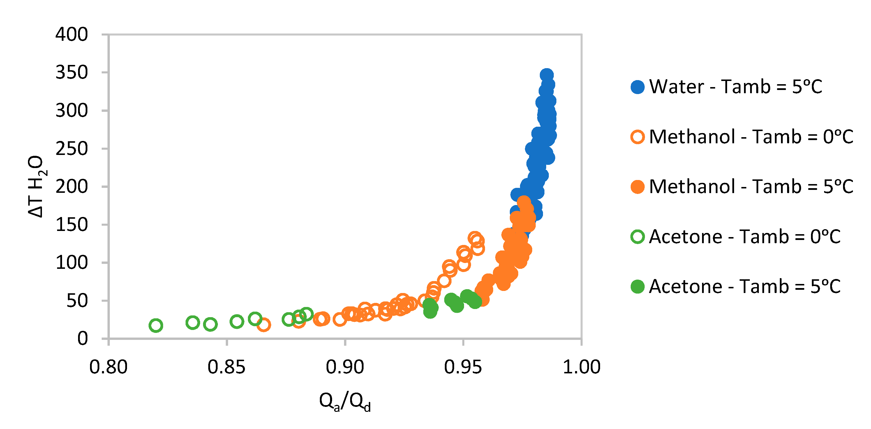
The whole range of absorbent pairs were simulated, and their results are shown in Figure 4, offering a general overview of how the water, methanol and acetone pairs modelled in this paper compare.

As can be observed in Figure 4, the performance of the acetone pair is lower than either water or methanol pairs and so its results are not be presented in any further detail below.

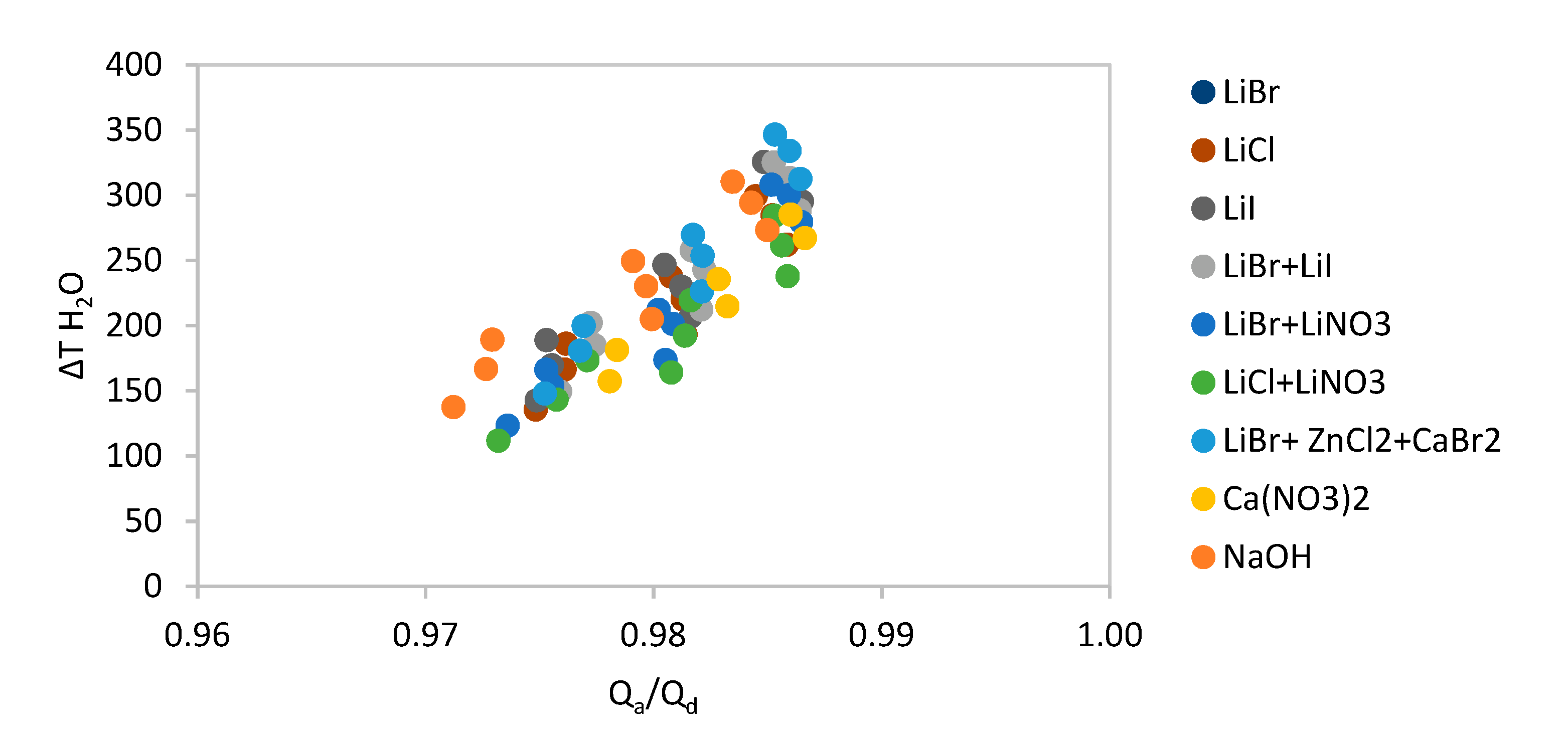
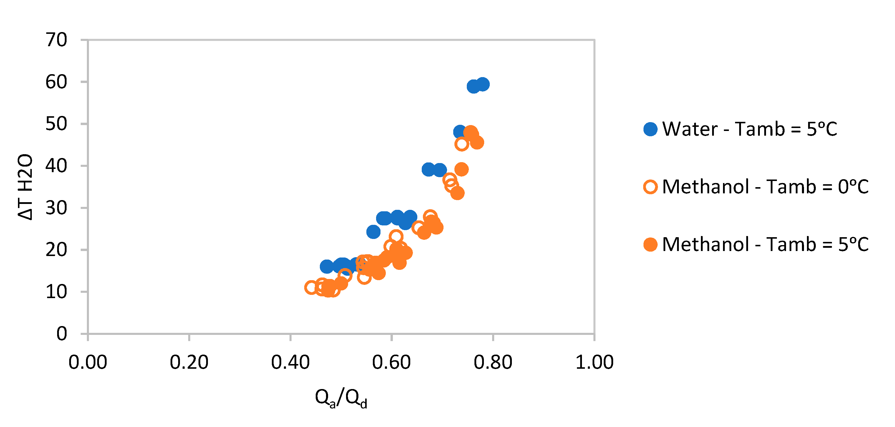
4.1.1. Water-Based Pairs

Figure 5 contains the performance of feasible water-based pairs suitable for an ambient temperature loop network. The different points correspond to a range of desorbing and absorbing temperatures $(T_a=8, 9, 10 °\mathrm{C}$ and $T_d=13, 14, 15 °\mathrm{C})$ but keeping the ambient temperature to 5 °C.

As can be observed, all the modelled pairs perform similarly and it can be concluded that on a simple thermal performance criterion there is little to choose between the pairs at these conditions.

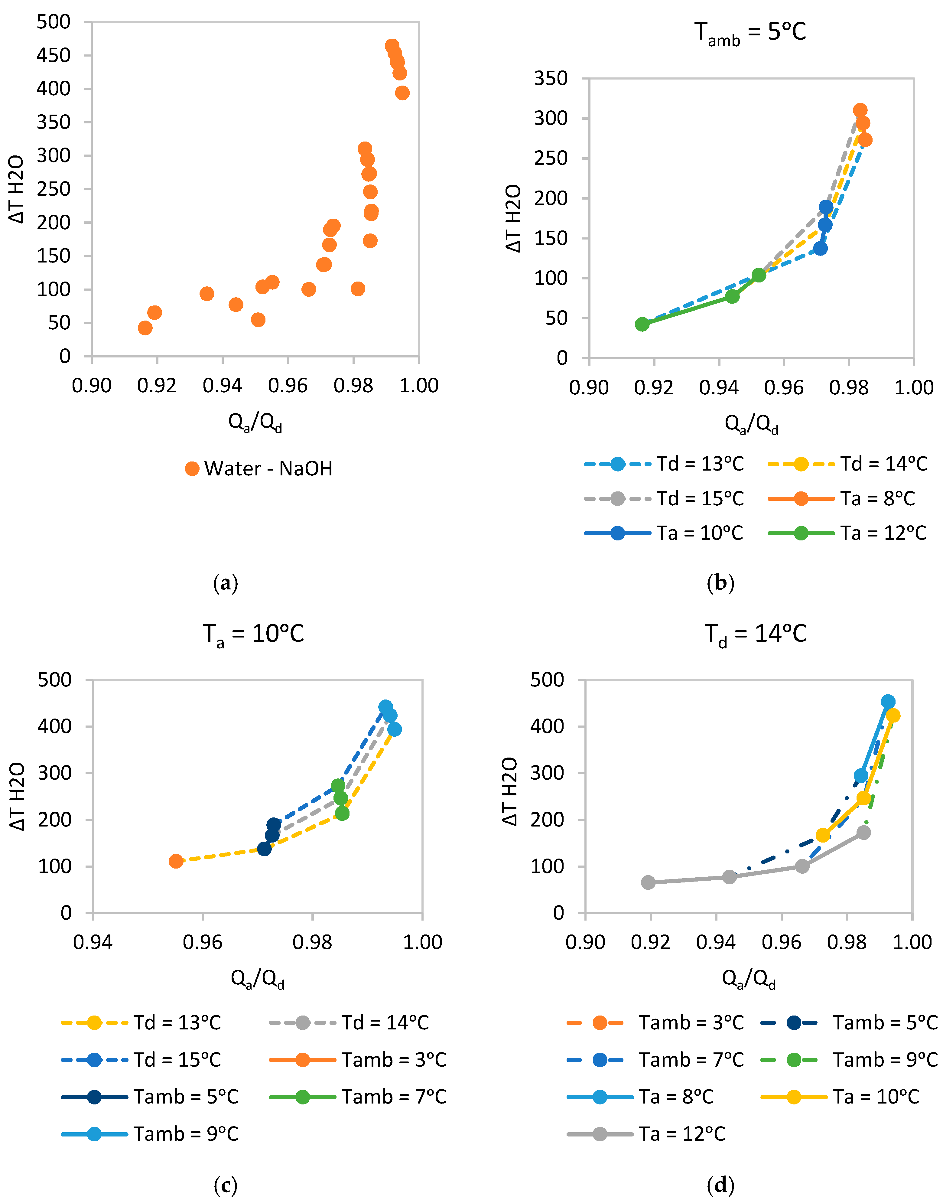
Nevertheless, sodium hydroxide (NaOH) has been chosen to be looked at in more detail since it performs relatively well and is a low cost material (much lower cost compared to salts that contain lithium). The performance points for $T_{amb}=3, 5, 7, 9 °\mathrm{C}$, $T_a=8, 10, 12 °\mathrm{C}$ and $T_d=13, 14, 15 °\mathrm{C}$ were obtained and plotted in Figure 6a. As can be observed, all the points present a very good Heat Ratio $\left(Q_a/Q_d\right)$ between 90 and 99%. On the other hand, the equivalent $\mathsf{\Delta }{T}_{H_{2}O}$ varies significantly between 40 and 465 °C.

Figure 6b–d disaggregate the combined data of Figure 6a to identify trends and understand the network performance.

Looking at Figure 6b–d trends can be observed but there is no ‘best result’ for an optimum $T_a$ and $T_d$ at a given $T_{amb}$.

When $T_{amb}$ is fixed, lower $T_a$ provide the best performance also enhanced with a choice of $T_d$ as close to $T_a$ as possible. A drawback of choosing a low $T_a$ is that the heat pumping technology of choice will have to upgrade heat to the user from a lower temperature level achieving a lower COP.

When $T_a$ is fixed, higher $T_{amb}$ provide the best performance, as expected, and as mentioned above, a choice of $T_d$ as close to $T_a$ as possible also improves the performance.

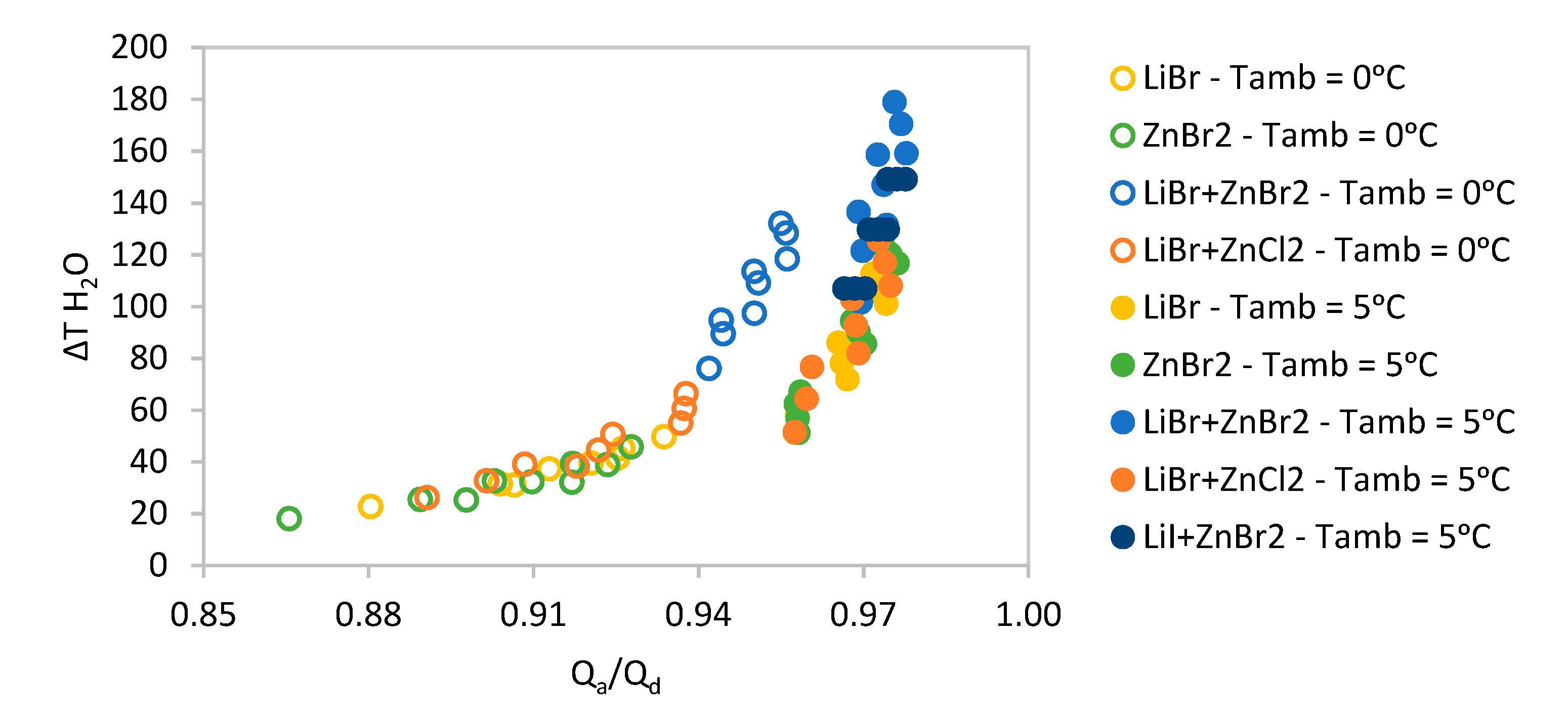
4.1.2. Methanol-Based Pairs

Figure 7 contains the performance of feasible methanol-based pairs suitable for an ambient temperature loop network. The different points correspond to a set range of desorbing and absorbing temperatures and they are divided into two groups: the hollow points correspond to an ambient temperature of 0 °C and the solid points correspond to an ambient temperature of 5 °C.

Although methanol-based pairs can be used at an ambient temperature of 0 °C, their ∆T and heat ratio drop quite significantly. At higher ambient temperatures $\left(T_{amb}=5 °\mathrm{C}\right)$ their performance is much lower compared to water-based pairs, as observed in Figure 7.

The best performing pair corresponds to CH₃OH-LiBr + ZnBr₂, as seen in Figure 7. Both $T_{amb}=0.5 °\mathrm{C}$ perform with heat ratios between 0.94 and 0.98 and ∆T between 80 and 180 °C (depending on $T_a$ and $T_d$ conditions).

4.1.3. Example Calculations for Ambient Loop Applications

In the following section the potential reduction of the network’s pipe size by using some of the modelled TC pairs has been calculated.

The example used is for a building heat demand of 3 MW that is being delivered by a conventional water heat district network (the approximated $\mathsf{\Delta }{T}_{H_{2}O}$ would be 10 °C). Assuming the specific heat of the water is constant and corresponds to $4.2 \mathrm{kJ}/\mathrm{kgK}$, it is possible to calculate the mass flow of water needed to deliver that heat:

$$\dot{Q}=c_p·\mathsf{\Delta }T·\dot{m}$$

(38)

$$\dot{m}=\raisebox{1ex}{$\dot{Q}$}\!\left/ \!\raisebox{-1ex}{$c_p·\mathsf{\Delta }T$}\right.=\raisebox{1ex}{$3·{10}^3$}\!\left/ \!\raisebox{-1ex}{$4.2·10$}\right.=71.43\raisebox{1ex}{$ \mathrm{kg}$}\!\left/ \!\raisebox{-1ex}{$\mathrm{s}$}\right.$$

This means the network needs two pipes (flow and return) that carry $71.5 \mathrm{kg}/\mathrm{s}\approx 71.5 \mathrm{l}/\mathrm{s}$ of water, $\approx 143 \mathrm{l}/\mathrm{s}$ in total.

Water–NaOH for Ambient Loop Applications

For a Water-Sodium Hydroxide pair working in an ambient loop temperature network desorbing at 14 °C, absorbing at 10 °C, and with an ambient temperature of 5 °C, the heating power delivered in the absorber would be 2494 kW with a 97% efficiency.

In order to deliver that heating power, the TC network would need to pump $4.28 \raisebox{1ex}{$\mathrm{l}$}\!\left/ \!\raisebox{-1ex}{$\mathrm{s}$}\right.$ of dilute solution, $3.15 \mathrm{l}/\mathrm{s}$ of concentrated solution and $1.20 \mathrm{l}/\mathrm{s}$ of water, being the total sum of mass flows $\approx 8.6 \mathrm{l}/\mathrm{s}$. This corresponds to approximately 6% of the original mass flow, using a pipe diameter approximately 75% smaller.

Methanol–LiBr + ZnBr₂ for Ambient Loop Application

For the same heat demand but instead using methanol as the refrigerant, the improvements would be lower but as mentioned earlier, methanol can work at lower ambient temperatures.

For a methanol–lithium bromide+zinc bromide pair working in the same ambient loop temperature network and with an ambient temperature of 5 °C, the heating power delivered in the absorber would be 1190 kW with a 97% efficiency. The mass flow pumped in the TC network would corresponds to approximately 8.5% of the originally mass flow, and it would use a pipe diameter approximately 71% smaller.

In the case of the same pair working with an ambient temperature of 0 °C, the mass flow pumped in the TC network would corresponds to approximately 11.2% of the originally mass flow, and it would use a pipe diameter approximately 66% smaller.

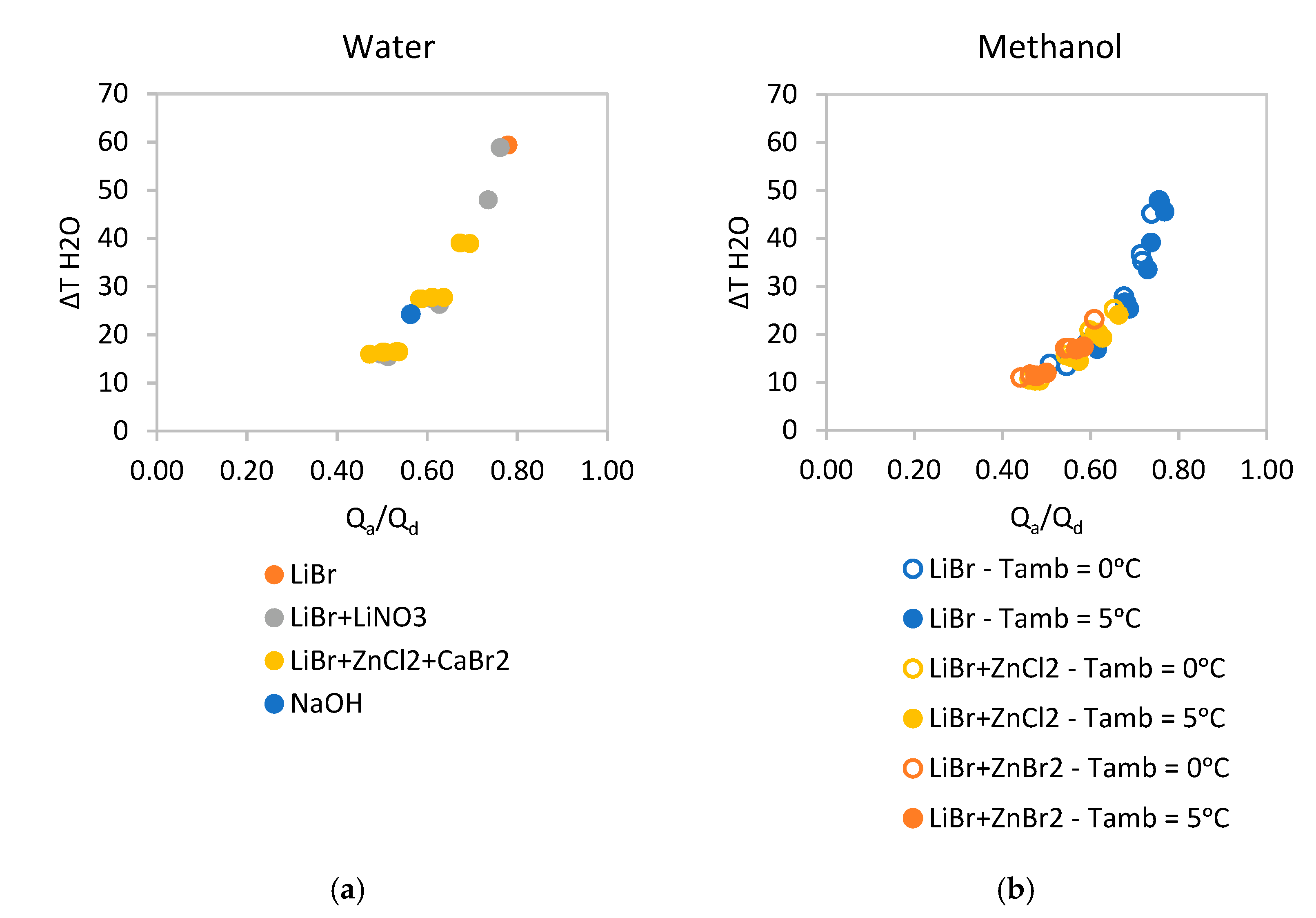
4.2. Network for High Temperature Loop

Similar to the ambient loop network, the high temperature network works between two higher desorption and absorption temperature levels (absorbing between 45 and 55 °C and desorbing between 2 and 10 °C above $T_a$). By doing this, the TC network can be used to produce useful heating in the delivery point (absorber) using a low temperature heat input to the desorber and having the advantage of not requiring insulated pipes.

The whole range of suitable absorbent pairs for these conditions were simulated and the results are shown in Figure 8.

Due to sary sitallization, not all the pairs presented previously are suitable for these temperature conditions and their performance is quite low. The two best performing water-based solutions are Lithium Bromide and Lithium Bromide + Lithium Nitrate as it can be observed in Figure 9a. In the case of methanol, the best performing solution is Lithium Bromide as it can be observed in Figure 9b.

4.2.1. Example Calculations for High Temperature Loop Applications

In the following section, the potential reduction of the network’s pipe size that can be potentially achieved by using some of the modelled TC pairs for a high temperature loop network has been calculated for the same example building heat demand presented above. As previously mentioned, the conventional network needs two pipes (flow and return) that carry $71.5 \mathrm{kg}/\mathrm{s}\approx 71.5 \mathrm{l}/\mathrm{s}$ of water, $\approx 143 \mathrm{l}/\mathrm{s}$ in total.

Water–LiBr + ZnCl₂ + CaBr₂ for High Temperature Loop Applications

For a water–lithium bromide + zinc chloride + calcium bromide pair working in a high temperature loop network desorbing at 55 °C, absorbing at 50 °C, and with an ambient temperature of 5 °C, the heating power delivered in the absorber would be 1854 kW with a 50% efficiency.

In order to deliver that heating power, the TC network would need to pump $26.48 \raisebox{1ex}{$\mathrm{l}$}\!\left/ \!\raisebox{-1ex}{$\mathrm{s}$}\right.$ of dilute solution, $25.49 \mathrm{l}/\mathrm{s}$ of concentrated solution and $1.62 \mathrm{l}/\mathrm{s}$ of water being the total sum of mass flows $\approx 53.6 \mathrm{l}/\mathrm{s}$. This corresponds to approximately 38% of the originally mass flow, using a pipe diameter approximately 38% smaller.

Methanol–LiBr for High Temperature Loop Applications

For the same heat demand but instead using methanol as the refrigerant, the performance is better than the water-based pair. It also has the added advantage of being able to work at lower ambient temperatures.

For a methanol–lithium bromide pair working in the same high temperature loop network and with an ambient temperature of 5 °C, the heating power delivered in the absorber would be 1239 kW with a 65% efficiency. The mass flow pumped in the TC network would corresponds to approximately 20% of the originally mass flow, and it would use a pipe diameter approximately 53% smaller.

In the case of the same pair working with an ambient temperature of 0 °C, the mass flow pumped in the TC network would corresponds to approximately 19% of the originally mass flow, and it would use a pipe diameter approximately 56% smaller.

5. Discussion

This paper seeks to evaluate possible sorption TC reactions that might be used in a district heating network. A closed system using water, alcohol or acetone as a low-pressure refrigerant that is absorbed or desorbed into a hydroxide, bromide or similar salt is proposed. The main difference with other published papers on this subject is the detailed presentation of the thermodynamic model of the thermochemical network and the range of absorption pairs considered.

Considering the modelled refrigerants, water is not suitable for ambient temperatures of 0 °C or below (freezing point). Methanol and acetone pair performance is not as good as water but they can be used below 0 °C ambient temperature. The Acetone-Zinc Bromide pair is not recommended.

Detailed simulation results for both ambient temperature loops and high temperature loops are presented along with example calculations which compare their capacity with conventional networks.

From the presented graphs it is possible to observe that the pairs with the best performance (heat ratio and $\mathsf{\Delta }{T}_{H_{2}O}$) both for ambient loop and high temperature networks are water pairs, due to water’s exceptionally high latent heat of vaporization. Heat ratios of 98% and $\mathsf{\Delta }{T}_{H_{2}O}$ of 200 °C are easily achievable for ambient temperature loops and heat ratios of 70% and $\mathsf{\Delta }{T}_{H_{2}O}$ of 40 °C for high temperature loops both working at ambient temperatures of 5 °C.

The next best performing pairs use methanol, which has the benefit that methanol can be used as a working fluid with evaporating temperatures below 0 °C. In the case of an ambient temperature of 5 °C, heat ratios of 97% and $\mathsf{\Delta }{T}_{H_{2}O}$ of 150 °C are obtained for ambient temperature loops and heat ratios of 70% and $\mathsf{\Delta }{T}_{H_{2}O}$ of 35 °C for high temperature loops. For an ambient temperature of 0 °C the performance drops significantly in ambient temperature loops and slightly in high temperature loops. Heat ratios of 94% and $\mathsf{\Delta }{T}_{H_{2}O}$ of 60 °C are obtained for ambient temperature loops and heat ratios of 70% and $\mathsf{\Delta }{T}_{H_{2}O}$ of 30 °C for high temperature loops.

Finally, the least well performing refrigerant is acetone. For ambient temperature loops at 5 °C heat ratios of 95% and $\mathsf{\Delta }{T}_{H_{2}O}$ of 45 °C are obtained and for ambient temperature loops at 0 °C the heat ratio achieved is 86% and $\mathsf{\Delta }{T}_{H_{2}O}$ of 25 °C.

Of the water-based pairs, water–NaOH has been chosen for further analysis and future experimental testing at the authors’ institution. It is attractive for ambient temperature loop applications, dramatically reducing the pipe size of the network by 75% (corresponds to approximately 6% of the original mass flow) and its cost makes it economically competitive. The only identified limitation is the evaporating temperature of the network if the ambient air is used as the heat source (ambient temperature should be above 0 °C). Ways to overcome this issue might include using a ground or aquifer heat source or the possible the use of water alcohol mixtures. Other water pairs perform very well but they are based on lithium compounds, which due to their price, make the cost of the network prohibitive.

In the case of high temperature networks, a few water and methanol-based solutions perform similarly, but their heat ratio and $\mathsf{\Delta }{T}_{H_{2}O}$ are substantially lower, not making them economically attractive enough to implement in a network.

In summary, a detailed thermodynamic model of a thermochemical heat distribution network has been presented, many potential absorption pairs have been modelled and one good performing and economically viable absorption pair has been identified.

References

1. Revesz, A.; Jones, P.; Dunham, C.; Davies, G.; Marques, C.; Matabuena, R.; Scott, J.; Maidment, G. Developing novel 5th generation district energy networks. Energy 2020, 201, 117389. [Google Scholar] [CrossRef]
2. Liu, Q.S.; Yabe, A.; Kajiyama, S.; Fukuda, K. A review of study on thermal energy transport system by synthesis and decomposition reactions of methanol. JSME Int. J. Ser. B Fluids Therm. Eng. 2002, 45, 473–480. [Google Scholar] [CrossRef] [Green Version]
3. Kang, B.H.; Yabe, A. Performance analysis of a metal-hydride heat transformer for waste heat recovery. Appl. Therm. Eng. 1996, 16, 677–690. [Google Scholar] [CrossRef]
4. Nasako, K.; Ito, Y.; Osumi, M. Intermittent heat transport using hydrogen absorbing alloys. Int. J. Hydrog. Energy 1998, 23, 815–824. [Google Scholar] [CrossRef]
5. Kang, Y.T.; Akisawa, A.; Sambe, Y.; Kashiwagi, T. Absorption heat pump systems for solution transportation at ambient temperature-STA cycle. Energy 2000, 25, 355–370. [Google Scholar] [CrossRef]
6. Wang, R.Z.; Lin, P.; Xia, Z.Z.; Ma, Q. Ammonia–water absorption cycle: A prospective way to transport low-grade heat energy over long distance. Int. J. Low-Carbon Technol. 2011, 6, 125–133. [Google Scholar] [CrossRef] [Green Version]
7. Geyer, P.; Buchholz, M.; Buchholz, R.; Provost, M. Hybrid thermo-chemical district networks–Principles and technology. Appl. Energy 2017, 186, 480–491. [Google Scholar] [CrossRef] [Green Version]
8. Geyer, P.; Delwati, M.; Buchholz, M.; Giampieri, A.; Smallbone, A.; Roskilly, A.P.; Buchholz, R.; Provost, M. Use cases with economics and simulation for thermo-chemical district networks. Sustainability 2018, 10, 599. [Google Scholar] [CrossRef] [Green Version]
9. Low, D.I.R.; Moelwyn-Hughes, E.A. The Heat Capacities of Acetone, Methyl Iodide and Mixtures Thereof in the Liquid State. Proc. R. Soc. London. Ser. A Math. Phys. Sci. 1962, 267, 384–394. [Google Scholar]
10. Ajib, S.; Karno, A. Thermophysical properties of acetone-zinc bromide for using in a low temperature driven absorption refrigeration machine. Heat Mass Transf. 2008, 45, 61–70. [Google Scholar] [CrossRef]
11. Felsing, W.A.; Durban, S.A. The vapor pressures, densities, and some derived quantities for acetone. J. Am. Chem. Soc. 1926, 48, 2885–2893. [Google Scholar] [CrossRef]
12. Goodwin, R.D. Methanol Thermodynamic Properties from 176 to 673 K at pressures to 700 bar. J. Phys. Chem. Ref. Data 1987, 16, 799–892. [Google Scholar] [CrossRef]
13. de Reuck, K.M.; Craven, R.J.B. Methanol, International Thermodynamic Tables of the Fluid State–12; Blackwell Scientific Publications: London, UK, 1993. [Google Scholar]
14. Popiel, C.O.; Wojtkowiak, J. Simple Formulas for Thermophysical Properties of Liquid Water for Heat Transfer Calculations (from 0 °C to 150 °C). Heat Transf. Eng. 1998, 19, 87–101. [Google Scholar] [CrossRef]
15. Pátek, J.; Šifner, O. Fast calculations of the properties of superheated steam from the saturation curve up to 600 °C and 30 MPa. Nucl. Eng. Des. 1994, 148, 515–520. [Google Scholar] [CrossRef]
16. Wagner, W.; Pruss, A. International Equations for the Saturation Properties of Ordinary Water Substance. Revised According to the International Temperature Scale of 1990. Addendum to J. Phys. Chem. Ref. Data 16, 893 (1987). J. Phys. Chem. Ref. Data 1993, 22, 783–787. [Google Scholar] [CrossRef] [Green Version]
17. Yuan, Z.; Herold, K.E. Specific Heat Measurements on Aqueous Lithium Bromide. HVACR Res. 2005, 11, 361–375. [Google Scholar] [CrossRef]
18. American Society of Heating, Refrigerating and Air-Conditioning Engineers. ASHRAE Handbook; American Society of Heating, Refrigerating and Air Conditioning Engineers: Atlanta, GA, USA, 1986. [Google Scholar]
19. Stankus, S.V.; Khairulin, R.A.; Gruzdev, V.A.; Verba, O.I. The Density of Aqueous Solutions of Lithium Bromide at High Temperatures and Concentrations. High Temp. 2007, 45, 429–431. [Google Scholar] [CrossRef]
20. Iyoki, S.; Ohmorl, S.; Uemura, T. Heat Capacities of the Water-Lithium Bromide-Lithium Iodide System. J. Chem. Eng. Data 1990, 35, 317–320. [Google Scholar] [CrossRef]
21. Iyoki, S.; Iwasaki, S.; Kuriyama, Y.; Uemura, T. Integral Enthalpies of Mixing for Water + Lithium Bromide + Lithium Iodide and Water + Lithium Chloride + Lithium Nitrate at 298.15 K. J. Chem. Eng. Data 1993, 38, 299–301. [Google Scholar] [CrossRef]
22. Iyoki, S.; Iwasaki, S.; Uemura, T. Vapor Pressures of the Water-Lithium Bromide-Lithium Iodide System. J. Chem. Eng. Data 1990, 35, 429–433. [Google Scholar] [CrossRef]
23. Iyoki, S.; Yamanaka, R.; Uemura, T. Physical and thermal properties of the water-lithium bromide-lithium nitrate system. Int. J. Refrig. 1993, 16, 191–200. [Google Scholar] [CrossRef]
24. Iyoki, S.; Uemura, T. Physical and thermal properties of the water-lithium bromide zinc chloride-calcium bromide system. Int. J. Refrig. 1989, 12, 272–277. [Google Scholar] [CrossRef]
25. Conde, M.R. Properties of aqueous solutions of lithium and calcium chlorides: Formulations for use in air conditioning equipment design. Int. J. Therm. Sci. 2004, 43, 367–382. [Google Scholar] [CrossRef]
26. Chaudhari, S.K.; Patil, K.R. Thermodynamic Properties of Aqueous Solutions of Lithium Chloride. Phys. Chem. Liq. 2002, 40, 317–325. [Google Scholar] [CrossRef]
27. Iyoki, S.; Tanaka, H.; Kuriyama, Y.; Uemura, T. Heat Capacity for the Water + Lithium Chloride + Lithium Nitrate System at Temperatures from 283.15 to 433.15 K. J. Chem. Eng. Data 1994, 39, 685–687. [Google Scholar] [CrossRef]
28. Iyoki, S.; Kuriyama, Y.; Tanaka, H.; Kira, K.; Okabe, T.; Uemura, T. Vapor-pressure measurements on (water + lithium chloride + lithium nitrate) at temperatures from 274.15 K to 463.15 K. J. Chem. Thermodyn. 1993, 25, 569–577. [Google Scholar] [CrossRef]
29. Chase, M.W., Jr. NIST-JANAF Thermochemical Tables, 4th ed.; American Institute of Physics: College Park, MD, USA, 1998; Volume 9. [Google Scholar]
30. Patil, K.R.; Chaudhari, S.K.; Katti, S.S. Thermodynamic Properties of Aqueous Solutions of Lithium Iodide: Simplified Method for Predicting the Enthalpies from the Vapor-Pressure Data. Appl. Energy 1991, 39, 189–199. [Google Scholar] [CrossRef]
31. Salavera, D.; Esteve, X.; Patil, K.R.; Mainar, A.M.; Coronas, A. Solubility, Heat Capacity, and Density of Lithium Bromide + Lithium Iodide + Lithium Nitrate + Lithium Chloride Aqueous Solutions at Several Compositions and Temperatures. J. Chem. Eng. Data 2004, 49, 613–619. [Google Scholar] [CrossRef]
32. Oakes, C.S.; Felmy, A.R.; Sterner, S.M. Thermodynamic properties of aqueous calcium nitrate {Ca(NO3)2} to the temperature 373 K including new enthalpy of dilution data. J. Chem. Thermodyn. 2000, 32, 29–54. [Google Scholar] [CrossRef]
33. Ewing, W.W.; Rogers, A.N. Calcium Nitrate. IV. Heats of Dilution of Solutions of Calcium Nitrate in Water. J. Am. Chem. Soc. 1933, 55, 3603–3609. [Google Scholar] [CrossRef]
34. Jain, S.K.; Singh, V.V.; Gupta, A.K.; Jain, A.K. Solution properties of concentrated solutions: Densities & refractive indices of calcium nitrate solutions. Indian J. Chem. 1984, 23, 808–811. [Google Scholar]
35. Ewing, W.W. Calcium nitrate. II. The vapor pressure-temperature relations of the binary system calcium nitrate-water. J. Am. Chem. Soc. 1927, 49, 1963–1973. [Google Scholar] [CrossRef]
36. Alexandrov, A.A. The Equations for Thermophysical Properties of Aqueous Solutions of Sodium Hydroxide. In Proceedings of the 14th International Conference on the Properties of Water and Steam, Kyoto, Japan, 29 August–3 September 2005. [Google Scholar]
37. Wilson, H.R.; McCabe, W.L. Specific heats and heats of dilution of concentrated sodium hydroxide solutions. Ind. Eng. Chem. 1942, 34, 558–566. [Google Scholar] [CrossRef]
38. Olsson, J.; Jernqvist, A.; Aly, G. Thermophysical Properties of Aqueous NaOH-H2O Solutions at High Concentrations. Int. J. Thermophys. 1997, 18, 779–793. [Google Scholar] [CrossRef]
39. Iedema, P.D. The Absorption Heat Pump with Lithium Bromide/Zinc Bromide/Methanol. Ph.D. Thesis, Delft University of Technology, Delft, The Netherlands, 1984. [Google Scholar]
40. Saravanan, R.; Maiya, M.P. Comparison of methanol-based working fluid combinations for a bubble pump-operated vapour absorption refrigerator. Int. J. Energy Res. 1998, 22, 715–731. [Google Scholar] [CrossRef]
41. Iyoki, S.; Takigawa, T.; Uemura, T. Thermal and physical properties of the methanol-lithium bromide-zinc chloride system. Int. J. Refrig. 1991, 14, 78–85. [Google Scholar] [CrossRef]
Figure 1. Basic heat transmission using absorption/desorption.
Energies 15 01449 g001
Figure 2. Proposed thermochemical heat transmission system.
Energies 15 01449 g002
Figure 3. Thermochemical network system schematic.
Energies 15 01449 g003
Figure 4. Water, methanol and acetone pairs performance for T a m b = 5   ° C , T a = 8 , 9 , 10   ° C and T d = 13 , 14 , 15   ° C .
Energies 15 01449 g004
Figure 5. Water-based pairs performance for T a m b = 5   ° C , T a = 8 ,   9 ,   10   ° C and T d = 13 ,   14 ,   15   ° C .
Energies 15 01449 g005
Figure 6. (a) Water–NaOH pair performance data points for T a m b = 3 ,   5 ,   7 ,   9   ° C , T a = 8 ,   10 ,   12   ° C and T d = 13 ,   14 ,   15   ° C , (b) Data points for T a m b = 5   ° C linked by T a and T d . (c) Water-NaOH pair performance data points for T d = 14   ° C linked by T a m b and T a , (d) Data points for T a = 10   ° C linked by T a m b and T d .
Energies 15 01449 g006
Figure 7. Methanol-based pairs performance for T a m b = 0 ,   5   ° C , T a = 8 ,   9 ,   10   ° C and T d = 13 ,   14 ,   15   ° C .
Energies 15 01449 g007
Figure 8. Performance of water and methanol pairs performance for T a m b = 0 ,   5   ° C , T a = 45 ,   50 ,   55   ° C and T d = T a + 2 ,   4 ,   6 ,   8 ,   10   ° C .
Energies 15 01449 g008
Figure 9. (a) Contains the performance of feasible water-based pairs at an ambient temperature of 5 °C and (b) Feasible methanol-based pairs. The different points correspond to a range of desorbing and absorbing temperatures ( T a = 45 ,   50 ,   55   ° C and T d = T a + 2 ,   4 ,   6 ,   8 ,   10   ° C ). In the case of water, the ambient temperature is 5 °C and in the case of the methanol two ambient temperatures were simulated, 5 and 0 °C.
Energies 15 01449 g009
Publisher’s Note: MDPI stays neutral with regard to jurisdictional claims in published maps and institutional affiliations.