Generalized Sliding Mode Observers for Simultaneous Fault Reconstruction in the Presence of Uncertainty and Disturbance

Abstract

In this paper, a generalized sliding mode observer design method is proposed for the robust reconstruction of sensors and actuators faults in the presence of both unknown disturbances and uncertainties. For this purpose, the effect of uncertainty and disturbance on the system has been considered in generalized state-space form, and the LMI tool is combined with the concept of an equivalent output error injection method to reduce the effects of them on the reconstruction process. The upper bound of the disturbance and uncertainty are minimized in the design of the sliding motion so that the reconstruction of the faults will be minimized. The design method is applied for actuator faults in the generalized state-space form, and then with some suitable filtering, the method extends as sensors and actuators coincidentally faults. Since in the proposed approach, the state trajectories do not leave the sliding manifold even in simultaneous sensors and actuators faults, then the faults are reconstructed based upon information retrieved from the equivalent output error injection signal. Due to the importance of the robust fault reconstruction in the wind energy conversion system (WECS), the proposed approach is successfully applied to a 5 MW wind turbine system. The simulation results verify the robust performances of the proposed approach in the presence of unknown perturbations and uncertainties.

1. Introduction

In recent decades, industrial processes are becoming more and more complex; thus, ensuring the operational reliability of these processes is an important task. Among them, fault detection and isolation (FDI) methods play a pivotal role in making the process reliable. The sensor and actuator faults are known as the most frequent faults that occur in many control systems such as satellite/aircraft [1,2], wind turbines [3,4], vehicles suspension system [5,6], offshore platforms [7], motor drives [8], power systems, and renewable energies [9,10]. In the event of a fault occurrence, the reliability and efficiency of the system are severely affected, and thus, the fault reconstruction is an important issue in the context of FDI approaches, and various types of research have been done in this field. However, when the system is subject to the uncertainty and disturbance, at the same time, identifying and reconstructing simultaneous sensor and actuator faults are still challenging issues that need to be addressed carefully.

In [11], a PI observer is proposed for fault estimation purposes based on convex structures and by employing nonquadratic Lyapunov functions. As a result, less conservative conditions in the form of LMIs are obtained. In [12], the sensor and actuator faults reconstruction problem is addressed by only considering the uncertainty in the model. In [13], the actuator fault reconstruction (AFR) problem is investigated by introducing two observers: one to estimate unknown inputs and the other to facilitate fault reconstruction. A particular kind of actuator faults in manipulator systems, i.e., joint luck failure, is considered in [14], and two kinds of reconfiguration schemes are proposed to cope with this issue. In [15], a fault-tolerant control technique is studied for electro-hydraulic actuators. In this reference, an unknown input observer is used to reconstruct sensor faults in the presence of disturbances. In [16], a fault-tolerant sliding mode controller was designed for a class of fuzzy T-S systems subject to actuator saturation, external disturbances, and time-varying delay. Sliding mode control is a variable structure control method that is well known in nonlinear system control. In [17], integral sliding mode control is proposed to a new five-dimensional four-wing hyper chaotic system with hidden attractor. An adaptive finite-time sliding mode control is proposed in [18] to construct a family of nine new chameleon chaotic systems subjected to uncertainties and disturbances. In [19], a new synchronous quasi-sliding mode control (QSMC) is studied for Rikitake chaotic system. A selection on switching surface and the existing of QSMC is also considered in this reference. A composite sliding mode observer is proposed in [20] to study multi-sensor fault diagnosis and active fault-tolerant control in a PMSM drive system. For the FDI of a class of uncertain Lipschitz nonlinear systems, an adaptive robust sliding mode observer (SMO) is proposed in [21], where both external disturbance and faults are considered. A second-order sliding mode observer is considered in [22] to reconstruct sensor faults in an air-path system of a heavy-duty diesel engine in the presence of disturbance. In [23], an adaptive estimation approach is proposed to recover the bias fault of sensors in a class of nonlinear systems subject to unstructured uncertainty. In [9], the fault detection and fault-tolerant control problem for multi-area power systems with sensor failures were considered using a descriptor form SMO. In [24], an adaptive SMO and a descriptive form observer are combined to reconstruct the sensor and actuator faults where the stability analysis was performed by the Lyapunov method. For a linear system with disturbance and time-varying delay, an adaptive estimation approach is presented in [25] for AFR. The problem of fault-tolerant controller design for a synchronization problem of complex dynamical networks subject to actuator faults and saturation was investigated in [26,27]. In [28], a time shift approach for AFR with a time-delay of output is introduced by using an SMO. For wind turbine faults detecting, a new technique is proposed in [29] as a signal reconstruction modeling technique. In the mentioned paper, to detect faults at an early stage, multiple indicators are also calculated. A new data-driven sensor FDI technique is presented in [30] using interval-valued data and an enhanced reconstruction approach to develop fault isolation. Various methods for a simultaneous actuator and sensor faults reconstruction have been proposed in the literature. Inspired by a singular system theory, a descriptor observer design is presented in [31] to reconstruct the actuator fault based on the transformed coordinate system. In [32], both faults are simultaneously reconstructed in a special class of nonlinear system described by the Takagi–Sugeno model. In [33], a new robust and simultaneous actuator and sensor faults estimation is proposed for a class of LPV systems described with polytopic representation where the parameters evolve in the hypercube domain.

Discrepancies between the actual process and its model such as model uncertainties and disturbances cause misleading of fault detection and reconstruction. The problem of simultaneous fault detection and reconstruction of sensors and actuators in the presence of both uncertainties and unknown disturbances has been addressed in this paper. A noticeable feature of the proposed approach is that the inherent differences between the effect of uncertainty and disturbance on the system have been considered in the design of sliding mode observers in a generalized state-space form when faults occur at both sensors and actuators coincidentally. This problem is efficiently addressed in this paper, where two different distribution matrices are incorporated to represent perturbations and uncertainties in the system. Then, LMI and the equivalent output error injection (EOEI) methods have been used to design a robust SMO. Since the state trajectories of SMO do not leave the sliding manifold in the presence of the uncertainties and disturbances, then the sensor and actuator faults are reconstructed based upon information retrieved from the equivalent output error injection signal. In order to verify the robust performances of the proposed approach, we applied it to a 5 MW wind turbine system. The wind energy conversion system (WECS) is a typical large and complex nonlinear system with random and intermittent wind force. In the electrical power system, the safety of electrical equipment is the basis for ensuring the stability and reliability. Fault reconstruction’s aim is to guarantee the security of electrical power system operation and industry production. For this reason, we proposed fault reconstruction to ensure the safe and efficient operation of wind turbines. The wind turbine systems actuators and sensors have the highest probability of failure, which has the greatest impact on the WECS safe and efficient operation. A robust fault-tolerant control for a Takagi–Sugeno fuzzy model is studied for the wind energy conversion system in [34].

The rest of this paper is organized as follows. Description of the system in the presence of an actuator and sensor fault, disturbances and uncertainties, and design of the proposed SMO are presented in Section 2. A robust AFR employing the EOEI approach is presented in Section 3. Sensor fault reconstruction is studied similar to the actuator fault method by introducing a new state in Section 4. Simulation results and concluding remarks are provided in Section 5.

2. Description of the Problem

We consider a class of uncertain systems in the presence of fault and disturbance given as:

$$\begin{array}{c}\hfill \begin{array}{c}\dot{z}\left(t\right)=Az\left(t\right)+Bu\left(t\right)+M\partial (t,y,u)+Dd\left(t\right)+F{f}_a\left(t\right)\hfill \\ y\left(t\right)=Cz\left(t\right)+F_s{f}_s\left(t\right)\hfill \end{array}\end{array}$$

(1)

where $B\in R^{n\times m}$, $A\in R^{n\times n}$, $C\in R^{p\times n}$, $M\in R^{n\times k}$, $D\in R^{n\times q}$, $F\in R^{n\times r}$, and $F_s\in R^{p\times l}$ denote the matrices of inputs, states, outputs, unknown bounded uncertainties, disturbances, actuator faults, and sensor faults, respectively. We assume $p\ge q$, $p\ge l$, $n>p\ge r$, and F and C are full column rank matrices. We also assume that $f_a\left(t\right)$ is a bounded unknown function indicating the fault of actuators, where $∥f_a\left(t\right)∥\le \alpha \left(t\right)$, and $\alpha$ is a known function. Furthermore, the unknown bounded function $\partial (t,y,u)$ denotes the system’s uncertainty and $∥\partial (t,y,u)∥\le \beta$, where $\beta >0$ is a known parameter. Moreover, $d\left(t\right)$ denotes the disturbance signal, which is bounded $∥d\left(t\right)∥\le d_0$, where $d_0$ is a positive constant.

Assumption 1.

It is assumed that $rank\left(CF\right)=rank\left(F\right)=r$ and the system with $(A,F,C)$ matrices has all its invariant zeros in the LHP.

It is important to note that $p<n$ implies that some states may not be observable. To cope with this issue, the following theorem is utilized to extract the observable and unobservable parts of the system in (1) with $f_s\left(t\right)=0$ where the matrix F only appears in the observable subsystem.

Theorem 1.

Assuming the conditions of Assumption 1 are satisfied and $f_s\left(t\right)=0$, then, there exist linear nonsingular transformations $\tilde{z}={\mathcal{T}}_b\overline{z}$ and $\overline{z}={\mathcal{T}}_{c}z$ such that:

$$\begin{array}{c}\hfill \tilde{A}=\left[\begin{array}{cc}{A}_1& A_2\\ A_3& A_4\end{array}\right],\tilde{C}=[0_{p\times (n-p)},\mathcal{T}],\tilde{F}=\left[\begin{array}{c}{0}_{r\times r}\\ F_2\end{array}\right]\end{array}$$

(2)

where $F_2=\left[\begin{array}{c}{0}_{(p-r)\times r}\\ F_{22}\end{array}\right]\in R^{r\times r}$ and $\mathcal{T}\in R^{p\times p}$ is orthogonal and nonsingular, $A_1\in R^{(n-p)\times (n-p)}$, ${\tilde{B}}^T=[B_1^T,B_2^T],{\tilde{D}}^T=[D_{1_{(n-p)\times q}}^T,D_{2_{p\times q}}^T],{\tilde{M}}^T=[M_{1_{(n-p)\times k}}^T,M_{2_{p\times k}}^T]$.

Proof. 

First, consider ${\mathcal{T}}_c={[N_c,C^T]}^T$, where columns of $N_c$ span the null space of C and are orthonormal. Then, one obtains:

$$\begin{array}{c}\hfill \begin{array}{c}\dot{\overline{z}}\left(t\right)=\underset{A_c}{\underbrace{{\mathcal{T}}_{c}A{\mathcal{T}}_c^{-1}}}\overline{z}\left(t\right)+\underset{B_c}{\underbrace{{\mathcal{T}}_{c}B}}u\left(t\right)+\underset{M_c}{\underbrace{{\mathcal{T}}_{c}M}}\partial (t,y,u)\hfill \\ +\underset{D_c}{\underbrace{{\mathcal{T}}_{c}D}}d\left(t\right)+\underset{F_c}{\underbrace{{\mathcal{T}}_{c}F}}{f}_a\left(t\right)\hfill \\ \overline{y}=\underset{C_c}{\underbrace{{\mathcal{T}}_c^{-1}C}}\overline{z}=\left[\begin{array}{cc}{0}_{(n-p)}& I_p\end{array}\right]\overline{z}.\hfill \end{array}\end{array}$$

(3)

It can be seen that only the last p states are present at the output. Now, considering $F_c=\left[\begin{array}{c}{f}_{1_{(r\times r)}}\\ f_{2_{(p\times r)}}\end{array}\right]$, we define a nonsingular linear transformation matrix ${\mathcal{T}}_b$ as:

$$\begin{array}{c}\hfill {\mathcal{T}}_b=\left[\begin{array}{cc}{I}_{(n-p)}& -f_1{\left(f_2^T{f}_2\right)}^{-1}{f}_2^T\\ 0_{p\times (n-p)}& {\mathcal{T}}^T\end{array}\right]\end{array}$$

(4)

where the QR decomposition of $f_2$ is used to obtain $\mathcal{T}$. Then, by using $\tilde{z}={\mathcal{T}}_b\overline{z}$, one obtains:

$$\begin{array}{c}\hfill \begin{array}{c}\dot{\tilde{z}}\left(t\right)=\tilde{A}\tilde{z}\left(t\right)+\tilde{B}u\left(t\right)+\tilde{M}\partial (t,y,u)+\tilde{D}d\left(t\right)+\tilde{F}{f}_a\left(t\right)\hfill \\ \tilde{y}\left(t\right)=\tilde{C}\tilde{z}\left(t\right)\hfill \end{array}\end{array}$$

(5)

where

$$\begin{array}{c}\hfill \begin{array}{c}\tilde{A}=\left[\begin{array}{cc}{A}_1& A_2\\ A_3& A_4\end{array}\right],\tilde{F}=\left[\begin{array}{c}{0}_{r\times r}\\ F_2\end{array}\right],\tilde{D}=\left[\begin{array}{c}{D}_1\\ D_2\end{array}\right]\hfill \\ \tilde{C}=\left[0_{p\times (n-p)},\mathcal{T}\right],\tilde{B}=\left[\begin{array}{c}{B}_1\\ B_2\end{array}\right],\tilde{M}=\left[\begin{array}{c}{M}_1\\ M_2\end{array}\right].\hfill \end{array}\end{array}$$

(6)

 □

The following SMO is considered:

$$\begin{array}{c}\hfill \begin{array}{c}\dot{\widehat{\tilde{z}}}\left(t\right)=\tilde{A}\widehat{\tilde{z}}\left(t\right)+\tilde{B}u\left(t\right)-{\tilde{G}}_l{e}_{\tilde{y}}\left(t\right)+{\tilde{G}}_{n}v\hfill \\ \widehat{\tilde{y}}\left(t\right)=\tilde{C}\widehat{\tilde{z}}\left(t\right).\hfill \end{array}\end{array}$$

(7)

where $\widehat{\tilde{y}}\left(t\right)$ and $\widehat{\tilde{z}}\left(t\right)$ denote the estimation of outputs and states, respectively. The output estimation error is represented by $e_{\tilde{y}}\left(t\right)=\widehat{\tilde{y}}\left(t\right)-\tilde{y}\left(t\right)$. Furthermore, the observer gains ${\tilde{G}}_n,{\tilde{G}}_l\in R^{n\times p}$ will be defined in the following.

The sliding variable v has a nonlinear discontinuous term to maintain the sliding motion, which is given as:

$$\begin{array}{c}\hfill v=\left\{\begin{array}{c}0,\forall e_{\tilde{y}}=0\hfill \\ -\rho (t,y,u){∥e_{\tilde{y}}∥}^{-1}{e}_{\tilde{y}},\forall e_{\tilde{y}}\ne 0\hfill \end{array}\right.\end{array}$$

(8)

where the upper bound for the fault plus uncertainty and disturbance is represented by the gain factor $\rho (t,y,u)\in R$.

The gain ${\tilde{G}}_n$ is chosen as:

$$\begin{array}{c}\hfill {\tilde{G}}_n=\left[\begin{array}{c}-L{\mathcal{T}}^T\\ {\mathcal{T}}^T\end{array}\right]P_0^{-1}\end{array}$$

(9)

where $P_0=P_0^T\in R^{p\times p}$ is a PDF design matrix that will be calculated in the following and L is defined as:

$$\begin{array}{c}\hfill L=\left[\begin{array}{cc}{L}_0& 0\end{array}\right]\in R^{(n-p)\times p}\end{array}$$

(10)

where $L_0\in R^{(n-p)\times (p-r)}$ is adjusted such that $(L_0{A}_{31}+A_1)$ is Hurwitz, where $A_{31}$ represents the first $p-q$ rows of $A_3$.

Now, the following theorem is recalled from [35].

Theorem 2.

Assume an observer dynamic as given in (7), a Lyapunov matrix $\tilde{P}$, and a matrix ${\tilde{G}}_l$ satisfying:

$$\begin{array}{c}\hfill \begin{array}{c}\tilde{P}=\left[\begin{array}{cc}{P}_1& P_{1}L\\ L^T{P}_1& {\mathcal{T}}^T{P}_0\mathcal{T}+L^T{P}_{1}L\end{array}\right]\hfill \\ {(\tilde{A}-{\tilde{G}}_l\tilde{C})}^T\tilde{P}+\tilde{P}(\tilde{A}-{\tilde{G}}_l\tilde{C})<0\hfill \end{array}\end{array}$$

(11)

where L defined in (10) and $P_1\in R^{(n-p)\times (n-p)}$. Then, the observation error $e\left(t\right)\stackrel{\Delta }{=}\widehat{\tilde{z}}\left(t\right)-\tilde{z}\left(t\right)$ is asymptotically stable.

Considering Assumption 1, it can be shown that there exists a stable sliding motion on the sliding surface given as [36]:

$$\begin{array}{c}\hfill S=\left\{\left.e\left(t\right)|\tilde{C}e\left(t\right)=0\right\}.\right.\end{array}$$

(12)

Then, one obtains:

$$\begin{array}{c}\hfill \begin{array}{c}\dot{e}\left(t\right)=(\tilde{A}-{\tilde{G}}_l\tilde{C})e\left(t\right)-\tilde{M}\partial (t,y,u)\hfill \\ -\tilde{D}d\left(t\right)-\tilde{F}{f}_a\left(t\right)+{\tilde{G}}_{n}v\hfill \end{array}.\end{array}$$

(13)

Lemma 1.

The error dynamics in (13) is bounded in the region Ω defined as:

$$\begin{array}{c}\hfill \Omega =\left\{e|∥e∥<2({\mu }_2\beta +{\mu }_1{d}_0)/\phantom{2({\mu }_2\beta +{\mu }_1{d}_0){\mu }_0}{\mu }_0\right\}\end{array}$$

(14)

where ${\mu }_0=-{\lambda }_{max}\left({\tilde{A}}_c\right)$, ${\mu }_1=∥\tilde{P}\tilde{D}∥,{\mu }_2=∥\tilde{P}\tilde{M}∥$, ${\tilde{A}}_c=-{({\tilde{G}}_l\tilde{C}-\tilde{A})}^T\tilde{P}-\tilde{P}({\tilde{G}}_l\tilde{C}-\tilde{A})$.

Proof. 

Define $V=e^T\tilde{P}e$. Then

$$\begin{array}{c}\hfill \begin{array}{c}\dot{V}=e^T{\tilde{A}}_{c}e-2e^T\tilde{P}\tilde{M}\partial (t,y,u)-2e^T\tilde{P}\tilde{D}d\left(t\right)\hfill \\ -2e^T\tilde{P}\tilde{F}{f}_a\left(t\right)+2e^T\tilde{P}{\tilde{G}}_{n}v\hfill \end{array}.\end{array}$$

(15)

From (16) and considering $∥\partial (t,y,u)∥\le \beta$ and $∥d\left(t\right)∥\le d_0$ and utilizing the Cauchy–Schwartz inequality, yield:

$$\begin{array}{c}\hfill \begin{array}{c}\dot{V}\le -{\mu }_0{∥e∥}^2+2∥e∥{\mu }_1{d}_0+2∥e∥{\mu }_2\beta -2e^T\tilde{P}\tilde{F}{f}_a\left(t\right)+2e^T\tilde{P}{\tilde{G}}_{n}v.\hfill \end{array}\end{array}$$

(16)

Using (6), (9), and (11), it is simply verified that $\tilde{P}\tilde{F}={\tilde{C}}^T{P}_0\tilde{C}\tilde{F}$ and $\tilde{P}{\tilde{G}}_n={\tilde{C}}^T$. Then, considering $e_{\tilde{y}}\left(t\right)=\tilde{C}e\left(t\right)=\tilde{C}\left(\tilde{z}\left(t\right)-z\left(t\right)\right)$, $∥f_a\left(t\right)∥\le \alpha$ and (8), one obtains:

$$\begin{array}{c}\hfill \begin{array}{c}\dot{V}\le 2∥e∥{\mu }_1{d}_0-{\mu }_0{∥e∥}^2+2∥e∥{\mu }_2\beta \hfill \\ -2\left(\rho (t,y,u)-\alpha (t,u)∥P_0\tilde{C}\tilde{F}∥\right)∥e_{\tilde{y}}∥\hfill \\ \le -∥e∥\left({\mu }_0∥e∥-2{\mu }_1{d}_0-2{\mu }_2\beta \right).\hfill \end{array}\end{array}$$

(17)

Therefore, if $∥e∥>2({\mu }_2\beta +{\mu }_1{d}_0)/\phantom{2({\mu }_2\beta +{\mu }_1{d}_0){\mu }_0}{\mu }_0$, then $\dot{V}<0$, and this implies that $e\left(t\right)$ will converge to the following bounded region:

$$\begin{array}{c}\hfill \Omega =\left\{e|∥e∥<(2{\mu }_1{d}_0+2{\mu }_2\beta )/\phantom{(2{\mu }_1{d}_0+2{\mu }_2\beta ){\mu }_0}{\mu }_0\right\}.\end{array}$$

(18)

 □

Now, we show that with the proper selection of $\rho (y,u,t)$, the sliding surface in (13) is reached in finite time. Define:

$$\begin{array}{c}\hfill {\mathcal{T}}_L=\left[\begin{array}{cc}{I}_{n-p}& L\\ 0& \mathcal{T}\end{array}\right].\end{array}$$

(19)

Using this transformation, the matrices in (6), (9), and (11) are converted to the following form:

$$\begin{array}{c}\hfill \begin{array}{c}\mathcal{A}={\mathcal{T}}_L\tilde{A}{\mathcal{T}}_L^{-1}=\left[\begin{array}{cc}{\mathcal{A}}_1& {\mathcal{A}}_2\\ {\mathcal{A}}_3& {\mathcal{A}}_4\end{array}\right],\mathcal{M}={\mathcal{T}}_L\tilde{M}=\left[\begin{array}{c}{\mathcal{M}}_1\\ {\mathcal{M}}_2\end{array}\right]\hfill \\ {\mathcal{G}}_n={\mathcal{T}}_L{\tilde{G}}_n=\left[\begin{array}{c}0\\ P_0^{-1}\end{array}\right],\mathcal{F}={\mathcal{T}}_L\tilde{F}=\left[\begin{array}{c}{0}_{(n-p)\times r}\\ {\mathcal{F}}_2\end{array}\right]\hfill \\ \mathcal{D}={\mathcal{T}}_L\tilde{D}=\left[\begin{array}{c}{\mathcal{D}}_1\\ {\mathcal{D}}_2\end{array}\right],\mathcal{C}=\tilde{C}{\mathcal{T}}_L^{-1}=[\begin{array}{cc}{0}_{p\times (n-p)}& I_p]\end{array}\hfill \\ \mathcal{P}={\left({\mathcal{T}}_L^{-1}\right)}^T\tilde{P}{\mathcal{T}}_L^{-1}=\left[\begin{array}{cc}{P}_1& 0\\ 0& P_0\end{array}\right]\hfill \end{array}\end{array}$$

(20)

where:

$$\begin{array}{c}\hfill \begin{array}{c}{\mathcal{A}}_1=A_1+L{A}_3,{\mathcal{M}}_1=M_1+L{M}_2,{\mathcal{D}}_1=D_1+L{D}_2\hfill \\ {\mathcal{A}}_3=\mathcal{T}{A}_3,{\mathcal{M}}_2=\mathcal{T}{M}_2,{\mathcal{D}}_2=\mathcal{T}{D}_2,{\mathcal{F}}_2=\mathcal{T}{F}_2.\hfill \end{array}\end{array}$$

(21)

Therefore, the error in (14) becomes:

$$\begin{array}{c}\hfill \begin{array}{c}{\dot{e}}_l\left(t\right)=\left(\mathcal{A}-{\mathcal{G}}_L\mathcal{C}\right)e_l\left(t\right)-\mathcal{M}\partial (t,y,u)-\mathcal{D}d\left(t\right)\hfill \\ -\mathcal{F}{f}_a\left(t\right)+{\mathcal{G}}_{n}v\hfill \end{array}\end{array}$$

(22)

where

$$\begin{array}{c}\hfill e_l={\mathcal{T}}_{L}e=\left[\begin{array}{c}{e}_1\\ e_{\tilde{y}}\end{array}\right],{\mathcal{G}}_L={\mathcal{T}}_L{G}_l=\left[\begin{array}{c}{\mathcal{G}}_{L1}\\ {\mathcal{G}}_{L2}\end{array}\right].\end{array}$$

(23)

Using this, (23) can be decomposed as:

$$\begin{array}{c}\hfill \begin{array}{c}{\dot{e}}_1\left(t\right)={\mathcal{A}}_1{e}_1\left(t\right)+\left({\mathcal{A}}_2-{\mathcal{G}}_{L1}\right)e_{\tilde{y}}\left(t\right)\hfill \\ -{\mathcal{M}}_1\partial (t,y,u)-{\mathcal{D}}_{1}d\left(t\right)s\hfill \\ {\dot{e}}_{\tilde{y}}\left(t\right)={\mathcal{A}}_3{e}_1\left(t\right)+\left({\mathcal{A}}_4-{\mathcal{G}}_{L2}\right)e_{\tilde{y}}\left(t\right)+P_0^{-1}v\hfill \\ -{\mathcal{M}}_2\partial (t,y,u)-{\mathcal{D}}_{2}d\left(t\right)-{\mathcal{F}}_2{f}_a\left(t\right).\hfill \end{array}\end{array}$$

(24)

The following theorem proposes a proper choice of $\rho$ to guarantee finite time convergence to the sliding surface S.

Theorem 3.

The error dynamic (23) reaches the sliding surface S in finite-time $T_s\le \frac{\sqrt{V\left(0\right)}}{{\eta }_0\sqrt{{\lambda }_{min}\left(P_0^{-1}\right)}}$ and stays there forever, if:

$$\begin{array}{c}\hfill \begin{array}{c}\rho (t,y,u)\ge ∥P_0{\mathcal{D}}_2∥d_0+∥P_0{\mathcal{M}}_2∥\beta +∥P_0{\mathcal{F}}_2∥\alpha +\hfill \\ 2∥P_0{\mathcal{A}}_3∥({\mu }_1{d}_0+{\mu }_2\beta )/{\mu }_0+{\eta }_0.\hfill \end{array}\end{array}$$

(25)

Proof. 

Define the candidate Lyapunov function $V=e_{\tilde{y}}^T{P}_0{e}_{\tilde{y}}$. Then:

$$\begin{array}{c}\hfill \begin{array}{c}\dot{V}=e_{\tilde{y}}^T\left(P_0({\mathcal{A}}_4-{\mathcal{G}}_{L2})+{({\mathcal{A}}_4-{\mathcal{G}}_{L2})}^T{P}_0\right)e_{\tilde{y}}+\hfill \\ 2e_{\tilde{y}}^T{P}_0{\mathcal{A}}_3{e}_1-2e_{\tilde{y}}^T{P}_0{\mathcal{F}}_{2}f-2e_{\tilde{y}}^T{P}_0{\mathcal{D}}_{2}d-\hfill \\ 2e_{\tilde{y}}^T{P}_0{\mathcal{M}}_2\partial +2e_{\tilde{y}}^{T}v\hfill \end{array}\end{array}$$

(26)

where $2e_{\tilde{y}}^{T}v=-2\rho ∥e_{\tilde{y}}∥$. Then, by using the Cauchy–Schwartz inequality, one gets:

$$\begin{array}{c}\hfill \dot{V}\le -2∥e_{\tilde{y}}∥\left(\begin{array}{c}\rho -∥P_0{\mathcal{A}}_3∥∥e_1∥-∥P_0{\mathcal{F}}_2∥\alpha -\hfill \\ ∥P_0{\mathcal{D}}_2∥d_0-∥P_0{\mathcal{M}}_2∥\beta \hfill \end{array}\right).\end{array}$$

(27)

From (15), (24), and (25) we conclude that $\rho -∥P_0{\mathcal{A}}_3∥∥e_1∥-∥P_0{\mathcal{M}}_2∥\beta -∥P_0{\mathcal{D}}_2∥d_0-∥P_0{\mathcal{F}}_2∥\alpha ={\eta }_0>0$ and $∥e_1∥<2({\mu }_2\beta +{\mu }_1{d}_0)/\phantom{2({\mu }_2\beta +{\mu }_1{d}_0){\mu }_0}{\mu }_0$. This results:

$$\begin{array}{c}\hfill \dot{V}\le -2{\eta }_0∥e_{\tilde{y}}∥\le -2{\eta }_0\sqrt{{\lambda }_{min}\left(P_0^{-1}\right)}\sqrt{V}.\end{array}$$

(28)

Therefore, using (29) and the finite-time stability theorem (see Theorem 4.2 of [37]), we conclude that the estimation error converges to zero, and the sliding motion reaches S in finite-time $T_s\le \frac{1}{{\eta }_0}\sqrt{\frac{V\left(0\right)}{{\lambda }_{min}\left(P_0^{-1}\right)}}$.  □

Now, an LMI-based approach is proposed to obtain an appropriate gain matrix ${\tilde{G}}_l$. In this regard, Theorem 2.2 requires finding a matrix $\tilde{P}$ that satisfies:

$$\begin{array}{c}\hfill {(\tilde{A}-{\tilde{G}}_l\tilde{C})}^T\tilde{P}+\tilde{P}(\tilde{A}-{\tilde{G}}_l\tilde{C})<0.\end{array}$$

(29)

As discussed in [36], an inequality of the form (30) can be alternatively solved by the following set of inequalities:

$$\begin{array}{c}\hfill \tilde{P}>0,{\tilde{A}}^T\tilde{P}+\tilde{P}\tilde{A}-{\tilde{C}}^T{U}^{-1}\tilde{C}+\tilde{P}Q\tilde{P}<0\end{array}$$

(30)

where $U\in R^{p\times p}$ and $Q\in R^{n\times n}$ are PSD matrices. Applying the Schur lemma, (31) is converted to the following LMI:

$$\begin{array}{c}\hfill \left[\begin{array}{cc}\tilde{P}\tilde{A}+{\tilde{A}}^T\tilde{P}-{\tilde{C}}^T{U}^{-1}\tilde{C}& \tilde{P}\\ \tilde{P}& -Q^{-1}\end{array}\right]<0.\end{array}$$

(31)

The matrix $\tilde{P}$ is obtained by solving the LMI (32), and then:

$$\begin{array}{c}\hfill {\tilde{G}}_l={\tilde{P}}^{-1}{\tilde{C}}^T{U}^{-1}.\end{array}$$

(32)

3. Robust Actuator Faults Reconstruction

In this part, assuming that the proposed SMO gains in (7) are well-designed, an efficient approach is proposed for a robust AFR procedure. Relying on the results of Theorem 2.3, one obtains that $e_{\tilde{y}}={\dot{e}}_{\tilde{y}}=0$ as $t\to \infty$. Then:

$$\begin{array}{cc}\hfill & {\dot{e}}_1\left(t\right)={\mathcal{A}}_1{e}_1\left(t\right)-{\mathcal{M}}_1\partial (t,y,u)-{\mathcal{D}}_{1}d\left(t\right)\hfill \\ \hfill & 0={\mathcal{A}}_3{e}_1\left(t\right)-{\mathcal{M}}_2\partial (t,y,u)-{\mathcal{D}}_{2}d\left(t\right)-{\mathcal{F}}_2{f}_a\left(t\right)+P_0^{-1}{v}_{eq}\hfill \end{array}$$

(33)

where $v_{eq}$ is obtained by approximating v in (8):

$$\begin{array}{c}\hfill v_{eq}=-\rho (t,y,u)e_{\tilde{y}}{\left(\epsilon +∥e_{\tilde{y}}∥\right)}^{-1}\end{array}$$

(34)

where $\epsilon >0$. From (34), one obtains:

$$\begin{array}{c}\hfill \begin{array}{c}{\dot{e}}_1\left(t\right)=\left(L{A}_3+A_1\right)e_1\left(t\right)-\left(M_1+L{M}_2\right)\partial (t,y,u)\hfill \\ -\left(D_1+L{D}_2\right)d\left(t\right)\hfill \\ 0=\mathcal{T}\left(\begin{array}{c}{A}_3{e}_1\left(t\right)-M_2\partial (t,y,u)-\hfill \\ D_{2}d\left(t\right)-F_2{f}_a\left(t\right)\hfill \end{array}\right)+P_0^{-1}{v}_{eq}.\hfill \end{array}\end{array}$$

(35)

This implies:

$$\begin{array}{c}\hfill P_0^{-1}{v}_{eq}=\mathcal{T}\left(\begin{array}{c}-A_3{e}_1\left(t\right)+M_2\partial (t,y,u)+\hfill \\ D_{2}d\left(t\right)+F_2{f}_a\left(t\right)\hfill \end{array}\right).\end{array}$$

(36)

Now, the goal is to minimize or eliminate the effects of disturbance and uncertainty signals on the AFR. To this end, the reconstruction signal is defined as:

$$\begin{array}{c}\hfill {\widehat{f}}_i=W{\mathcal{T}}^T{P}_0^{-1}{v}_{eq}\end{array}$$

(37)

where $W=[W_1,F_{22}^{-1}]$. Multiplication of both sides in (37) by $W{\mathcal{T}}^T$ implies:

$$\begin{array}{c}\hfill {\widehat{f}}_i\left(t\right)=+f_a\left(t\right)-W{A}_3{e}_1\left(t\right)+[W{D}_2,W{M}_2]\left[\begin{array}{c}d\left(t\right)\\ \partial (t,y,u)\end{array}\right].\end{array}$$

(38)

From (36), we have:

$$\begin{array}{c}\hfill \begin{array}{c}{e}_1\left(s\right)=-{\left(sI-\left(L{A}_3+A_1\right)\right)}^{-1}\times \hfill \\ \left[L{D}_2+D_1,L{M}_2+M_1\right]\left[\begin{array}{c}d\left(t\right)\\ \partial (t,y,u)\end{array}\right].\hfill \end{array}\end{array}$$

(39)

Substitution of (40) in (39) results:

$$\begin{array}{c}\hfill \begin{array}{c}{\widehat{f}}_i\left(t\right)=f_a\left(t\right)+G\left(s\right)\left[\begin{array}{c}d\left(t\right)\\ \partial (t,y,u)\end{array}\right]\hfill \\ G\left(s\right)=\left[\begin{array}{cc}W{D}_2& W{M}_2\end{array}\right]+\hfill \\ W{A}_3{\left(sI-\left(L{A}_3+A_1\right)\right)}^{-1}\times \hfill \\ \left[\begin{array}{cc}L{D}_2+D_1& L{M}_2+M_1\end{array}\right].\hfill \end{array}\end{array}$$

(40)

Therefore, the effect of $\left[\begin{array}{c}d\left(t\right)\\ \partial (t,y,u)\end{array}\right]$ on the fault reconstruction signal will be minimized or bounded if:

$$\begin{array}{c}\hfill {∥G\left(s\right)∥}_{\infty }<\xi \end{array}$$

(41)

where $\xi$ is a small constant. Let define $\tilde{P}$ in (31) as:

$$\begin{array}{c}\hfill \tilde{P}=\left[\begin{array}{cc}{\tilde{P}}_{11}& {\tilde{P}}_{12}\\ {\tilde{P}}_{12}^T& {\tilde{P}}_{22}\end{array}\right]>0\end{array}$$

(42)

where ${\tilde{P}}_{22}\in R^{p\times p}$ and ${\tilde{P}}_{11}\in R^{(n-p)\times (n-p)}$. By applying the Bounded Real Lemma (BRL) [38], the inequality (42) is converted to:

$$\begin{array}{c}\hfill \begin{array}{c}\left[\begin{array}{ccc}{\Phi }_{11}& {\Phi }_{12}& -{\left(W{A}_3\right)}^T\\ {\Phi }_{12}^T& -\xi I& {\left(W\left[\begin{array}{cc}{D}_2& M_2\end{array}\right]\right)}^T\\ -W{A}_3& W\left[\begin{array}{cc}{D}_2& M_2\end{array}\right]& -\xi I\end{array}\right]<0\hfill \\ {\Phi }_{11}={\tilde{P}}_{11}{A}_1+A_1^T{\tilde{P}}_{11}+{\tilde{P}}_{12}{A}_3+A_3^T{\tilde{P}}_{12}^T\hfill \\ {\Phi }_{12}=-({\tilde{P}}_{11}\left[\begin{array}{cc}{D}_1& M_1\end{array}\right]+{\tilde{P}}_{12}\left[\begin{array}{cc}{D}_2& M_2\end{array}\right]).\hfill \end{array}\end{array}$$

(43)

By solving (44), one obtains W and $\tilde{P}$. Then, by substituting W in (38) results:

$$\begin{array}{c}\hfill {\widehat{f}}_i\left(t\right)\simeq f_a\left(t\right).\end{array}$$

(44)

4. Robust Sensor Fault Reconstruction

In this case and without loss of generality, we define a new state $y_n\left(t\right)\in R^p$ that converts (1) with $f_a\left(t\right)=0$ to a similar form presented in the previous section, i.e., (1) with $f_s\left(t\right)=0$, so that a similar algorithm can be used. To this aim, let us define:

$$\begin{array}{c}\hfill {\dot{y}}_n\left(t\right)+A_n{y}_n\left(t\right)=A_{n}y\left(t\right)\end{array}$$

(45)

where $A_n$ is a stable PD matrix. Then, one obtains:

$$\begin{array}{c}\hfill {\dot{y}}_n\left(t\right)=-A_n{y}_n\left(t\right)+A_{n}Cz\left(t\right)+A_n{F}_s{f}_s\left(t\right).\end{array}$$

(46)

Now, an augmented system with $n+p$ states is defined as:

$$\begin{array}{cc}\hfill & \left[\begin{array}{c}\dot{z}\left(t\right)\\ {\dot{y}}_n\left(t\right)\end{array}\right]=\underset{A_N}{\underbrace{\left[\begin{array}{cc}A& 0\\ A_{n}C& -A_n\end{array}\right]}}\left[\begin{array}{c}z\left(t\right)\\ y_n\left(t\right)\end{array}\right]+\underset{B_N}{\underbrace{\left[\begin{array}{c}B\\ 0\end{array}\right]}}u\left(t\right)\hfill \\ \hfill & +\underset{F_N}{\underbrace{\left[\begin{array}{c}0\\ A_n{F}_s\end{array}\right]}}{f}_s\left(t\right)+\underset{D_N}{\underbrace{\left[\begin{array}{c}D\\ 0\end{array}\right]}}d\left(t\right)+\underset{M_N}{\underbrace{\left[\begin{array}{c}M\\ 0\end{array}\right]}}\partial (t,y,u)\hfill \\ \hfill & y_n\left(t\right)=\underset{C_N}{\underbrace{\left[\begin{array}{cc}0& I_p\end{array}\right]}}\left[\begin{array}{c}z\left(t\right)\\ y_n\left(t\right)\end{array}\right].\hfill \end{array}$$

(47)

Using this augmented model, it is evident that the sensor fault reconstruction (SFR) can be handled similar to the AFR procedure discussed in the previous section.

5. Simultaneous Sensor and Actuator Faults Reconstruction

In this section, a more general case is investigated where the sensor and actuator faults occur simultaneously, i.e., $f_s\left(t\right)\ne 0$ and $f_a\left(t\right)\ne 0$. Before proceeding to the main results, some precalculations need to be done. As discussed earlier, the nonsingular transformation matrices $H={[H_1,H_2]}^T$ and $\mathcal{T}$ exist such that:

$$\begin{array}{c}\hfill \begin{array}{c}\mathcal{T}A{\mathcal{T}}^{-1}=\left[\begin{array}{cc}{A}_1& A_2\\ A_3& A_4\end{array}\right],\mathcal{T}B=\left[\begin{array}{c}{B}_1\\ 0\end{array}\right],\hfill \\ \mathcal{T}{F}_a=\left[\begin{array}{c}{F}_{a_1}\\ 0\end{array}\right],\mathcal{T}D=\left[\begin{array}{c}{D}_1\\ 0\end{array}\right],\mathcal{T}M=\left[\begin{array}{c}{M}_1\\ 0\end{array}\right],\hfill \\ HC{\mathcal{T}}^{-1}=\left[\begin{array}{cc}{C}_1& 0\\ 0& C_4\end{array}\right],H{F}_s=\left[\begin{array}{c}0\\ F_{s_2}\end{array}\right].\hfill \end{array}\end{array}$$

(48)

Then, the system (1) in the new coordinates $\overline{z}=\mathcal{T}z=\left[\begin{array}{c}{\overline{z}}_1\\ {\overline{z}}_2\end{array}\right]$ and $\overline{y}=Hy=\left[\begin{array}{c}{\overline{y}}_1\\ {\overline{y}}_2\end{array}\right]$ is decomposed as

$$\begin{array}{cc}\hfill & \left\{\begin{array}{c}{\dot{\overline{z}}}_1\left(t\right)=A_1{\overline{z}}_1\left(t\right)+A_2{\overline{z}}_2\left(t\right)+B_{1}u\left(t\right)\hfill \\ +F_{a_1}{f}_a\left(t\right)+D_{1}d\left(t\right)+M_1\partial (t,y,u)\hfill \\ {\overline{y}}_1\left(t\right)=C_1{\overline{z}}_1\left(t\right)\hfill \end{array}\right.\hfill \end{array}$$

(49)

$$\begin{array}{cc}\hfill & \left\{\begin{array}{c}{\dot{\overline{z}}}_2\left(t\right)=A_3{\overline{z}}_1\left(t\right)+A_4{\overline{z}}_2\left(t\right)\hfill \\ {\overline{y}}_2\left(t\right)=C_4{\overline{z}}_2\left(t\right)+F_{s_2}{f}_s\left(t\right)\hfill \end{array}.\right.\hfill \end{array}$$

(50)

By defining ${\overline{z}}_3=\left[\begin{array}{c}{\overline{z}}_2\hfill \\ f_s\hfill \end{array}\right]$ and $C_5=\left[\begin{array}{cc}{C}_4& F_{s_2}\end{array}\right]$, Equation (51) can be rewritten as:

$$\begin{array}{c}\hfill \begin{array}{c}N{\dot{\overline{z}}}_3={\overline{A}}_3{\overline{z}}_1+{\overline{A}}_4{\overline{z}}_3+{\overline{F}}_{s_2}{f}_s\hfill \\ {\overline{y}}_2=C_5{\overline{z}}_3\hfill \end{array}\end{array}$$

(51)

where

$$\begin{array}{cc}\hfill & \left\{\begin{array}{c}{\dot{\overline{z}}}_1\left(t\right)=A_1{\overline{z}}_1\left(t\right)+A_2{\overline{z}}_2\left(t\right)+B_{1}u\left(t\right)\hfill \\ +F_{a_1}{f}_a\left(t\right)+D_{1}d\left(t\right)+M_1\partial (t,y,u)\hfill \\ {\overline{y}}_1\left(t\right)=C_1{\overline{z}}_1\left(t\right)\hfill \end{array}\right.\hfill \end{array}$$

(52)

$$\begin{array}{cc}\hfill & \left\{\begin{array}{c}{\dot{\overline{z}}}_2\left(t\right)=A_3{\overline{z}}_1\left(t\right)+A_4{\overline{z}}_2\left(t\right)\hfill \\ {\overline{y}}_2\left(t\right)=C_4{\overline{z}}_2\left(t\right)+F_{s_2}{f}_s\left(t\right)\hfill \end{array}\right..\hfill \end{array}$$

(53)

Considering ${\overline{A}}_2=[A_2,0]$, from (50) one obtains:

$$\begin{array}{c}\hfill \begin{array}{c}{\dot{\overline{z}}}_1\left(t\right)=A_1{\overline{z}}_1\left(t\right)+{\overline{A}}_2{\overline{z}}_3\left(t\right)+B_{1}u\left(t\right)+F_{a_1}{f}_a\left(t\right)\hfill \\ +D_{1}d\left(t\right)+M_1\partial (t,y,u)\hfill \end{array}.\end{array}$$

(54)

Combining (50)–(54), we get:

$$\begin{array}{cc}\hfill & \left\{\begin{array}{c}{\dot{\overline{z}}}_1\left(t\right)=A_1{\overline{z}}_1\left(t\right)+{\overline{A}}_2{\overline{z}}_3\left(t\right)+B_{1}u\left(t\right)\hfill \\ +F_{a_1}{f}_a\left(t\right)+K_1\psi (t,y,u)\hfill \\ {\overline{y}}_1\left(t\right)=C_1{\overline{z}}_1\left(t\right)\hfill \end{array}\right.\hfill \end{array}$$

(55)

$$\begin{array}{cc}\hfill & \left\{\begin{array}{c}N{\dot{\overline{z}}}_3={\overline{A}}_3{\overline{z}}_1+{\overline{A}}_4{\overline{z}}_3+{\overline{F}}_{s_2}{f}_s\hfill \\ {\overline{y}}_2=C_5{\overline{z}}_3\hfill \end{array}\right.\hfill \end{array}$$

(56)

where $K_1=[D_1,M_1],{\overline{K}}_2=[{\overline{D}}_2,{\overline{M}}_2],\psi (t,y,u)=\left[\begin{array}{c}d\left(t\right)\\ \partial (t,y,u)\end{array}\right]$. Based on the above results, the following theorem characterizes the proposed method for simultaneous reconstruction of the sensor and actuator faults in the presence of disturbances and uncertainties.

Theorem 4.

Consider the faulty system (55) and (56), and assume the observer structure as:

$$\begin{array}{cc}\hfill & \begin{array}{c}\left(N+V{C}_5\right)\dot{x}=\left({\overline{A}}_4-L_1{C}_5\right)x+L_2\left(y_1-C_1{\widehat{\overline{z}}}_1\right)\hfill \\ +{\overline{A}}_3{\widehat{\overline{z}}}_1+{\overline{A}}_4{\left(N+V{C}_5\right)}^{-1}V{y}_2\hfill \end{array}\hfill \end{array}$$

(57)

$$\begin{array}{cc}\hfill & {\widehat{\overline{z}}}_3=x+{(N+V{C}_5)}^{-1}V{y}_2\hfill \end{array}$$

(58)

$$\begin{array}{cc}\hfill & {\dot{\widehat{\overline{z}}}}_1=A_1{\widehat{\overline{z}}}_1+{\overline{A}}_2{\widehat{\overline{z}}}_3+B_{1}u\left(t\right)+{\overline{G}}_{n}v\left(t\right)-{\overline{G}}_l{e}_{y_1}.\hfill \end{array}$$

(59)

Then, the observer error is bounded if there exist $P_1=P_1^T$, $P_3=P_3^T$, and K satisfying the following LMIs

$$\begin{array}{c}\hfill \underset{Q}{\underbrace{\left[\begin{array}{ccc}{Q}_{11}& P_1{\overline{A}}_2& P_{1}K\\ *& Q_{22}& Q_{23}\\ *& *& -I\end{array}\right]}}<0\end{array}$$

(60)

$$\begin{array}{c}\hfill P_1>0,P_3>0\end{array}$$

(61)

where ⁎ denotes the transpose of each symmetric element, and

$$\begin{array}{c}\hfill \begin{array}{c}{Q}_{11}=A_1^T{P}_1+P_1{A}_1+{\lambda }^2{∥{\mathcal{T}}^{-1}∥}^2{I}_m,\hfill \\ Q_{23}=P_3{\left(N+V{C}_5\right)}^{-1}\hfill \\ Q_{22}=Q_{23}{\overline{A}}_4-K{C}_5-{\overline{A}}_4^T{Q}_{23}^T-C_5^T{K}^T\hfill \\ +{\lambda }^2{∥{\mathcal{T}}^{-1}∥}^2{I}_{n+p-2m}\hfill \end{array}.\end{array}$$

(62)

Furthermore, the observer error bound is given as follows

$$\begin{array}{c}\hfill ∥e∥<\sigma =2{\lambda }_{min}^{-1}\left(Q\right)∥P_3\left[\begin{array}{c}0\\ {\left(V_2{\overline{F}}_{s_2}\right)}^{-1}\end{array}\right]∥+{\sigma }_0\end{array}$$

(63)

where ${\sigma }_0$ is a small positive scalar.

Proof. 

For the observer (57)–(59), with $e_{y_1}={\widehat{y}}_1-y_1=C_1{e}_1$ we have:

$$\begin{array}{cc}\hfill & v\left(t\right)=-{\rho }_0\left({\widehat{\overline{z}}}_1-{\overline{z}}_1\right){\left(∥\left({\widehat{\overline{z}}}_1-{\overline{z}}_1\right)∥\right)}^{-1}\hfill \end{array}$$

(64)

$$\begin{array}{cc}\hfill & \begin{array}{c}{L}_2={\overline{A}}_3{C}_1^{-1}\hfill \\ L_1=\left(N+V{C}_5\right)P_{3}K\hfill \end{array}\hfill \end{array}$$

(65)

where ${\rho }_0$ is a positive scalar. Defining $e_1={\widehat{\overline{z}}}_1-{\overline{z}}_1$, $e_3={\widehat{\overline{z}}}_3-{\overline{z}}_3$ and using (57)–(59) one obtains:

$$\begin{array}{c}\hfill \begin{array}{c}{\dot{e}}_1=\left(A_1-{\overline{G}}_l{C}_5\right)e_1+{\overline{A}}_2{e}_3-F_{a_1}{f}_a\left(t\right)\hfill \\ +{\overline{G}}_{n}v\left(t\right)-K_1\psi (t,y,u)\hfill \\ {\dot{e}}_3=-\underset{{Q^{\prime }}_{23}}{\underbrace{Q_{23}{\overline{A}}_4{\left(N+V{C}_5\right)}^{-1}}}{e}_3-Q_{23}{\overline{F}}_{s_2}{f}_s\hfill \end{array}.\end{array}$$

(66)

Defining $s\left(t\right)=e_1\left(t\right)$ and $V=\frac{1}{2}{s}^T{P}_{1}s$, we get:

$$\begin{array}{c}\hfill \dot{V}\le ∥P_1{e}_1∥\left(\begin{array}{c}∥\left(A_1-{\overline{G}}_l{C}_5\right)e_1+{\overline{A}}_2{e}_3∥-{\rho }_0{\overline{G}}_n\hfill \\ -∥F_{a_1}{f}_a\left(t\right)∥-∥K_1\psi (t,y,u)∥\hfill \end{array}\right)\end{array}$$

(67)

where ${\overline{G}}_{n}v\left(t\right)=-{\rho }_0{\overline{G}}_n{e}_1{∥e_1∥}^{-1}$. Choosing ${\rho }_0\ge ∥{\overline{G}}_n^{-1}∥\left(l∥\left(A_1-{\overline{G}}_l{C}_5\right)∥+∥{\overline{A}}_2∥-∥F_{a_1}∥-∥K_1∥\right)\epsilon$, implies that after a finite time, we have $e_1\left(t\right)={\dot{e}}_1\left(t\right)=0$. Then, one obtains

$$\begin{array}{c}\hfill 0={\overline{A}}_2{e}_3-F_{a_1}{f}_a\left(t\right)+{\overline{G}}_{n}v\left(t\right)-K_1\psi (t,y,u).\end{array}$$

(68)

Now, the following actuator reconstruction signal is defined:

$$\begin{array}{c}\hfill {\widehat{f}}_a=W{\overline{G}}_n{v}_{eq}\left(t\right)\end{array}$$

(69)

where $W=F_{a_1}^{-1}$. To preserve sliding motion, $v\left(t\right)$ must take in the average $v_{eq}\left(t\right)=-{\rho }_0{e}_1{\left(∥e_1∥+\epsilon \right)}^{-1}$. Then, multiplying (68) by W results:

$$\begin{array}{c}\hfill {\widehat{f}}_a=-W{\overline{A}}_2{e}_3+f_a\left(t\right)+W{K}_1\psi (t,y,u).\end{array}$$

(70)

Then, one obtains

$$\begin{array}{c}\hfill \begin{array}{c}{\widehat{f}}_a-f_a=-W{\overline{A}}_2{e}_3+\underset{Z}{\underbrace{W{K}_1}}\psi (t,y,u)\hfill \\ \to ∥{\widehat{f}}_a-f_a∥<{\upsilon }^{\prime }+∥Z∥\psi (t,y,u)\hfill \end{array}\end{array}$$

(71)

where ${\upsilon }^{\prime }>∥W{\overline{A}}_2{e}_3∥$ is a small positive constant. Assuming ${∥Z∥}_{\infty }<{\upsilon }^{″}$ with ${\upsilon }^{″}>0$, results:

$$\begin{array}{c}\hfill ∥{\widehat{f}}_a-f_a∥<\upsilon .\end{array}$$

(72)

For small $\upsilon$, it implies ${\widehat{f}}_a\approx f_a$. Then, from (66) one obtains

$$\begin{array}{c}\hfill {\dot{e}}_3+Q_{23}^{\prime }{e}_3=\sigma =-Q_{23}{\overline{F}}_{s_2}{f}_s.\end{array}$$

(73)

Now, the following sensor reconstruction signal is defined:

$$\begin{array}{c}\hfill {\widehat{f}}_s=W_s\sigma \end{array}$$

(74)

where $W_s={\left(-Q_{23}{\overline{F}}_{s_2}\right)}^{-1}$. Then, one obtains

$$\begin{array}{c}\hfill ∥{\widehat{\overline{z}}}_3-{\overline{z}}_3∥\le \sigma .\end{array}$$

(75)

This implies ${\widehat{f}}_s\approx f_s$ and completes the proof.  □

Remark 1.

Regarding the design parameters tuning, it is worthwhile to mention some points. The parameter ε in (34) should be initially selected as a very small scalar and then gradually increased such that it approximates the output error injection v and fulfills the design requirements. The parameter ξ in (41) is a small constant that satisfies the LMI conditions (43).

Remark 2.

In practice, both sensor and actuator faults may occur simultaneously. Therefore, unlike most existing approaches dealing with sensor and actuator faults separately, our proposed approach takes care of simultaneous sensor and actuator faults, which can be a critical issue in some systems such as aircraft, wind turbines, etc., which need some more technical cares to have much better performance and efficiency.

The step-by-step procedure of applying the proposed design algorithm is summarized as follows:

(I): 

Use (2) and (4) to obtain the new coordinate system as defined in Theorem 2.1 (${\mathcal{T}}_c,{\mathcal{T}}_b$, and $\mathcal{T}$ are obtained).

(II): 

In the case of robust AFR, solve the LMI (44) to obtain $\tilde{P}$, which minimizes the effects of disturbances and uncertainties. Then, design the observer gains using (9) and (33). Finally, the actuator fault is reconstructed using (38).

(III): 

In the case of robust SFR, first construct the augmented system equations proposed in (48). Then, apply (I) and (II) to the augmented system to solve SFR.

(IV): 

In the case of simultaneous sensor and AFR, first use (49) to obtain the new coordinate system.

(V): 

Considering the proposed observer structure in Theorem 5.1, solve the LMIs (60) and (61) to obtain $P_1,P_3$, and K. Then, design the observer gains using (64) and (65). Finally, the actuator and sensor faults are reconstructed using (69) and (74).

6. Simulation Results

To verify the effectiveness of the proposed approaches, we consider a 5 MW wind turbine subject to the actuator and sensor faults in the presence of disturbances and uncertainties. The model and the parameters of the wind turbine used in the simulations are taken from [4] as following:

$$\begin{array}{c}\hfill \begin{array}{c}\dot{x}\left(t\right)=Ax\left(t\right)+Bu\left(t\right)+Dd\left(t\right)+M\partial (t,y)+F{f}_a\left(t\right)\hfill \\ y\left(t\right)=Cx\left(t\right)+F_s{f}_s\left(t\right)\hfill \\ A=\left[\begin{array}{ccccc}0& 1.0000& -0.0406& 0& 0\\ -88.8900& -0.8889& 0.0361& 6.685e-45& 0\\ 32552& 325.2& -13.22& 0& -0.1\\ 0& 0& 0& -6.6670& 0\\ 0& 0& 0& 0& -10\end{array}\right],B=F=\left[\begin{array}{cc}0& 0\\ 0& 0\\ 0& 0\\ 10& 0\\ 0& 6.6667\end{array}\right]\hfill \\ C=\left[\begin{array}{ccccc}0& 1& 0& 0& 0\\ 0& 0& 1& 0& 0\\ 0& 0& 0& 1& 0\end{array}\right],D=\left[\begin{array}{c}1\\ 0\\ 1\\ 0\\ 1\end{array}\right],M=\left[\begin{array}{c}1\\ -0.5\\ 1\\ 0\\ 0\end{array}\right],F_s=\left[\begin{array}{ccc}1& 0& 0\\ 0& 1& 0\\ 0& 0& 1\end{array}\right].\hfill \end{array}\end{array}$$

The state and the control input vectors are denoted as

$$\begin{array}{cc}\hfill x\left(t\right)& ={\left[\begin{array}{ccccc}\Theta \left(t\right)& {\Omega }_r\left(t\right)& {\Omega }_g\left(t\right)& \beta \left(t\right)& T_g\left(t\right)\end{array}\right]}^T\hfill \\ \hfill u\left(t\right)& ={\left[\begin{array}{cc}{\beta }_r\left(t\right)& T_{g,d}\left(t\right)\end{array}\right]}^T\hfill \end{array}$$

(76)

where $\Theta \left(t\right)$ the torsion angle, ${\Omega }_r\left(t\right)$ the rotor speed, ${\Omega }_g\left(t\right)$ the generator speed, $\beta \left(t\right)$ the pitch angle, and $T_g\left(t\right)$ the generator torque are the state variables and $T_{g,d}\left(t\right)$ the desired generator torque and ${\beta }_r\left(t\right)$ the pitch angle command are the control input of the wind turbine model.

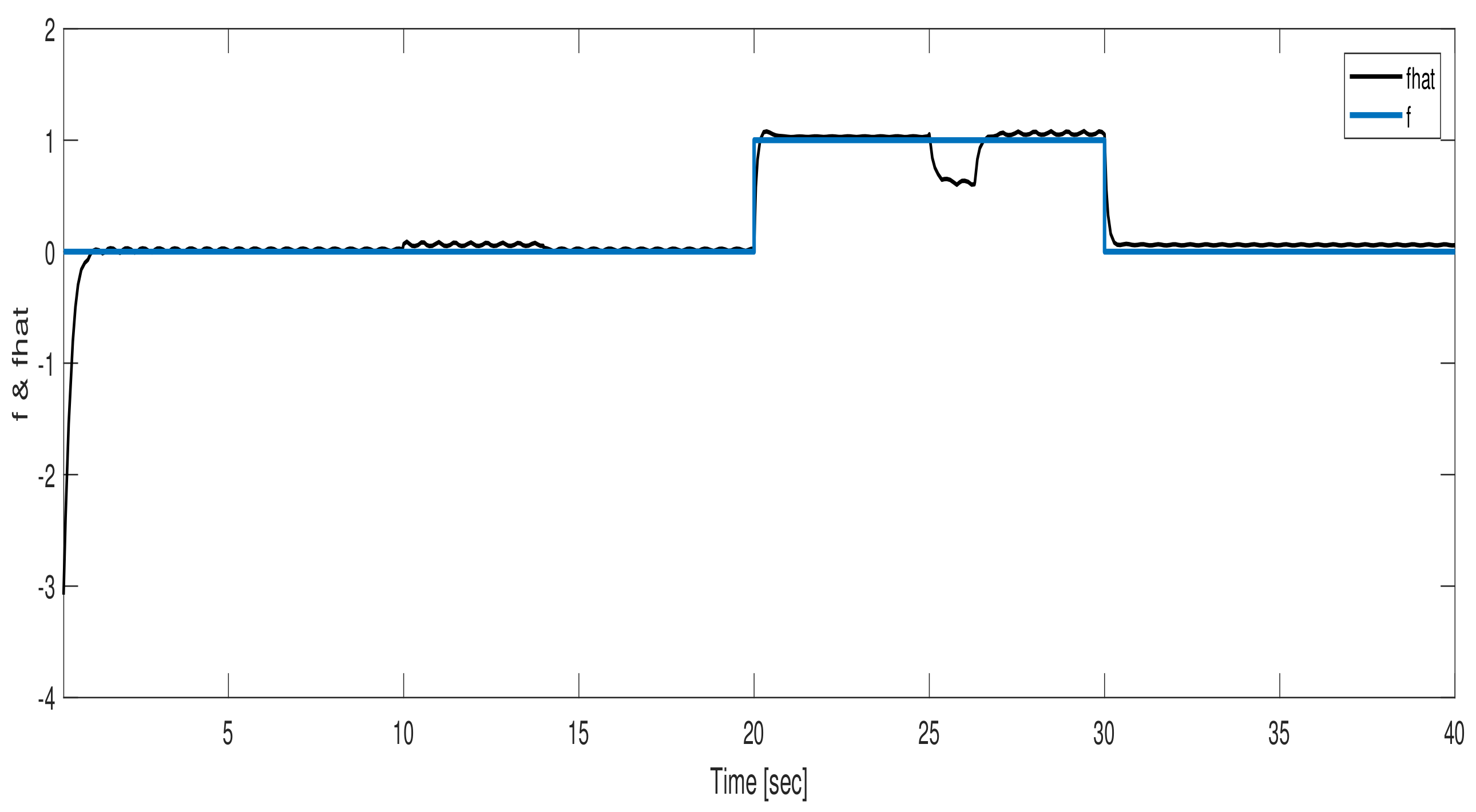
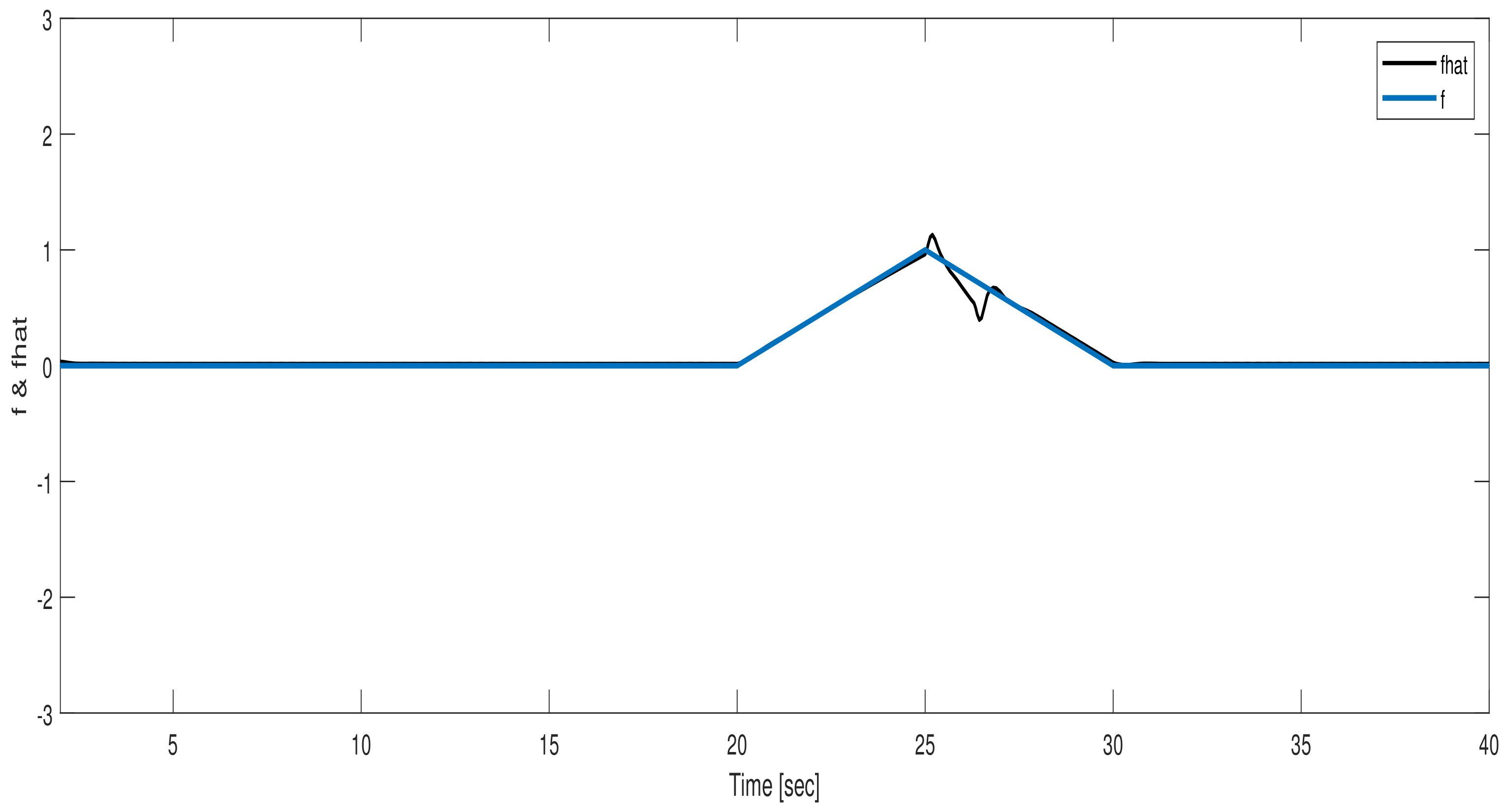
6.1. Actuator Fault Reconstruction

First, the following stabilizing controller is designed:

$$\begin{array}{c}\hfill u\left(t\right)=\left[\begin{array}{ccccc}-14.34& -1.26& -0.01& 0.33& -3.06\\ 21.89& 0.28& 0.07& -0.82& 9.37\end{array}\right]x\left(t\right).\end{array}$$

During the simulation, we assume $x\left(0\right)={\left[0.5,1,1,1.5,0.5\right]}^T$; the disturbance $d\left(t\right)=u(t-25)$ and the uncertainty $\partial (t,y,u)=\left[0,0.5,2\right]y$ are also considered. It is easy to check that Assumption 1 is satisfied for this system, so the proposed method is applicable. Using the results in Theorem 2, the transformation matrix ${\mathcal{T}}_b$ is calculated as:

$$\begin{array}{c}\hfill T_b=\left[\begin{array}{ccccc}1& 0& 0& 0& 0\\ 0& 1& 0& 0& 0\\ 0& 0& 0& 1& 0\\ 0& 0& -1& 0& 0\\ 0& 0& 0& 0& -1\end{array}\right].\end{array}$$

Then, the LMI (44) is solved to minimize the effects of disturbances and uncertainties. Consequently, the observer gains and the AFR are obtained using (9), (33), and (38) as:

$$\begin{array}{c}\hfill G_l=\left[\begin{array}{ccc}-0.1& -3.3& 0\\ 0.01& 0.1& 0\\ -1.55& 71.6& 0\\ -0.8& 1.55& 0\\ 0& 0& -0.1\end{array}\right],G_n=\left[\begin{array}{ccc}-0.001& 0.07& 0\\ 0.001& -0.07& 0\\ 2.75& 2.68& 0\\ 1.37& 1.3& 0\\ 0& 0& -0.13\end{array}\right].\end{array}$$

The associated matrices L and $P_0$ are calculated as:

$$\begin{array}{c}\hfill L=\left[\begin{array}{ccc}1& 1& 0\\ -1& -1& 0\\ 0& -1& 1\end{array}\right],P_0=\left[\begin{array}{ccc}-13.35& 14.06& 0\\ 14.06& -14.05& 0\\ 0& 0& 7.53\end{array}\right].\end{array}$$

The Lyapunov matrix P is also obtained from (30):

$$\begin{array}{c}\hfill P=\left[\begin{array}{ccccc}8.41& 0& 0.1& -0.8& 0\\ 0& 5.65& -0.01& 0& 0\\ 0.1& 0& 0& -0.1& 0\\ -0.81& 0& -0.1& 0.72& 0\\ 0& 0& 0& 0& 7.53\end{array}\right].\end{array}$$

The parameters $\epsilon$ and $\rho$ are selected as 0.5 and 10, respectively. Then, choosing $\xi =1\times {10}^{-3}$, the matrix W is calculated as $W=\left[-0.676,-0.581,-0.28\right]$.

Figure 1 and Figure 2 show the effectiveness of the proposed AFR algorithm reconstructing faults simultaneously occurring in both actuators in the presence of the mentioned unknown disturbances/uncertainties.

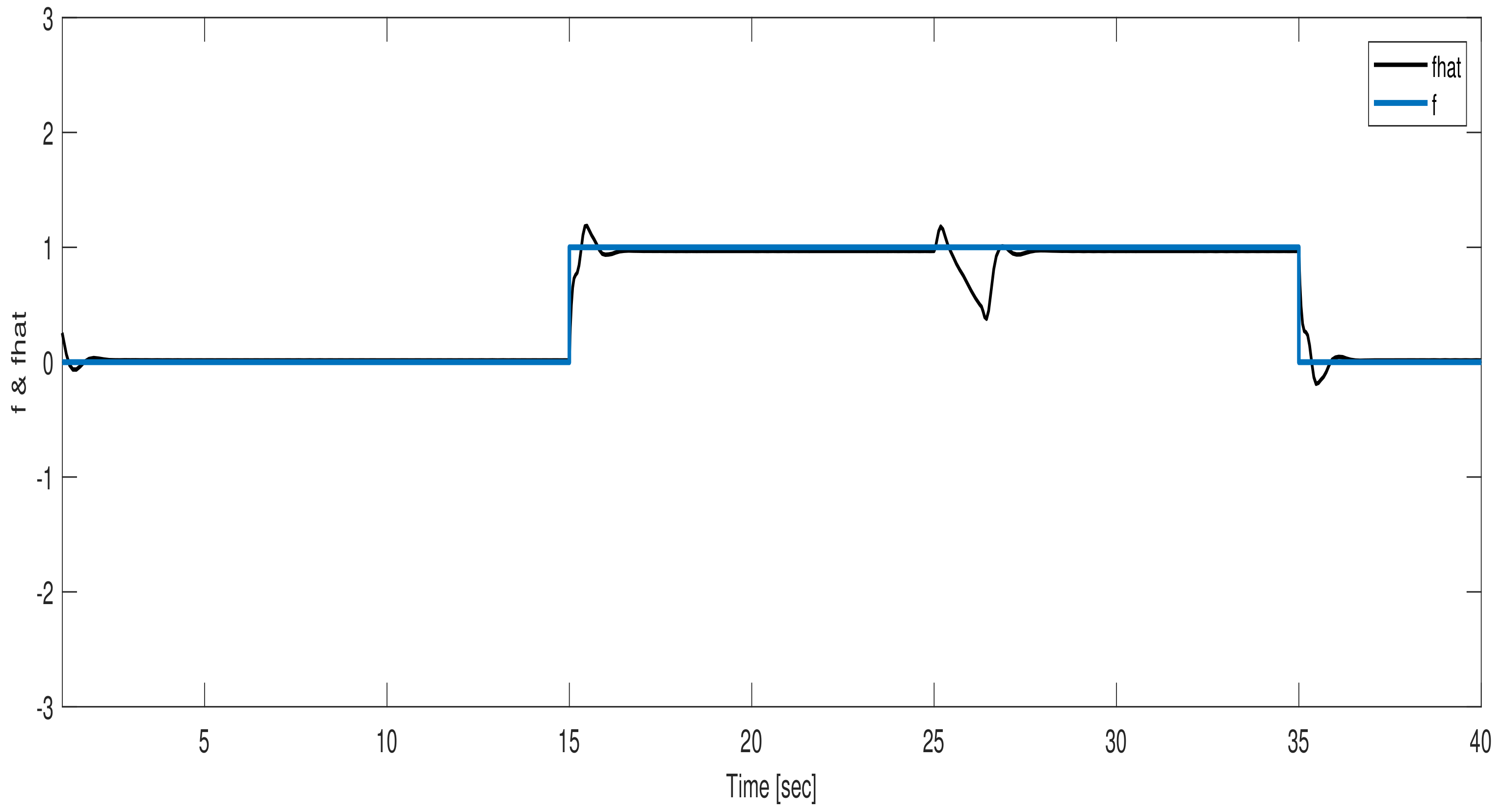
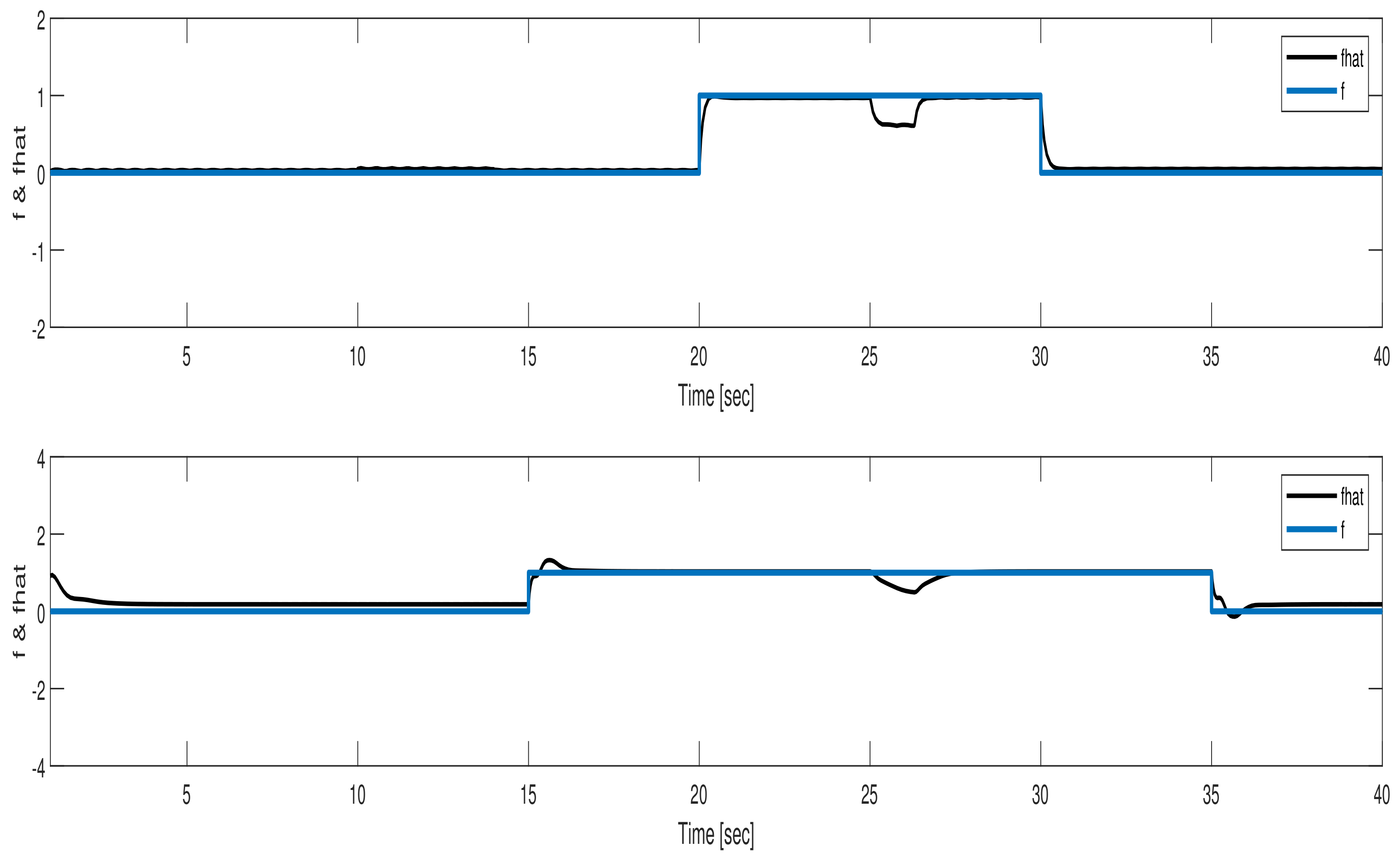
6.2. Sensor Fault Reconstruction

First, by choosing $A_n=20I_{3\times 3}$, the matrices of the associated augmented model in (48) are obtained.

$$\begin{array}{c}\hfill \begin{array}{c}A=\left[\begin{array}{cccccccc}0& 1& 0& 0& 0& 0& 0& 0\\ 8.9& -1& 0& 0& 0& 0& 0& 0\\ 25.5& 32.25& -13& 0& 0& 0& 0& 0\\ 0& 0& 0& -7& 0& 0& 0& 0\\ 0& 0& 0& -10& 0& 0& 0& 0\\ 0& 0& 0& 0& -20& 0& 0& 0\\ 0& 20& 0& 0& 0& -20& 0& 0\\ 0& 0& 20& 0& 0& 0& -20& 0\end{array}\right],B=\left[\begin{array}{cc}0& 0\\ 0& 0\\ 0& 0\\ 10& 0\\ 0& 6.68\\ 0& 0\\ 0& 0\\ 0& 0\end{array}\right]\hfill \\ C=\left[\begin{array}{cccccccc}0& 0& 0& 0& 0& 1& 0& 0\\ 0& 0& 0& 0& 0& 0& 1& 0\\ 0& 0& 0& 0& 0& 0& 0& 1\end{array}\right],D=\left[\begin{array}{c}1\\ 0\\ 1\\ 0\\ 1\\ 0\\ 0\\ 0\end{array}\right],M=\left[\begin{array}{c}1\\ 0.5\\ 1\\ 0\\ 0\\ 0\\ 0\\ 0\end{array}\right],F_s=\left[\begin{array}{c}0\\ 0\\ 0\\ 0\\ 0\\ 0\\ 0\\ 20\end{array}\right].\hfill \end{array}\end{array}$$

Then, using a similar procedure the matrix $T_b$ is obtained as:

$$\begin{array}{c}\hfill T_b=\left[\begin{array}{cccccccc}1& 0& 0& 0& 0& 0& 1& 0\\ 0& 1& 0& 0& 0& 0& 0& 1\\ 0& 0& 1& 0& 0& 0& 0& 0\\ 0& 0& 0& 1& 0& 0& 0& 0\\ 0& 0& 0& 0& 1& 0& 0& 1\\ 0& 0& 0& 0& 0& 0& -1& 0\\ 0& 0& 0& 0& 0& 1& 0& 0\\ 0& 0& 0& 0& 0& 0& 0& -1\end{array}\right].\end{array}$$

Using this coordinate transformation, the equivalent model is obtained. Then, a stabilizing controller is designed as $u\left(t\right)=Kz\left(t\right)$, where:

$$\begin{array}{c}\hfill K=\left[\begin{array}{cccccccc}-201.7& -10.1& -0.1& 2.7& -0.1& 1.3& -8.4& 56\\ -4214.3& -6& -18.7& 31.5& 0.3& 1.2& -188.2& 84.4\end{array}\right].\end{array}$$

In this case, we assume $x\left(0\right)={[1,0.5,1,0.5,1.5,1,2,0.5]}^T$, $\partial (t,y,u)=\left[0.3,-0.5,0\right],y=0.3z_5-0.5z_6$, and $d\left(t\right)=u(t-20)$. Using a similar procedure, the observer gains are obtained for the augmented system as:

$$\begin{array}{c}\hfill G_n=\left[\begin{array}{ccc}-0.1& 0& -0.16\\ 0& -0.1& 0.16\\ -0.01& 0& -0.43\\ -0.01& -0.01& 0.3\\ 0& 0& 0.3\\ 0& -0.01& -1.3\\ -1.3& 0& 1.3\\ -1.3& -0.3& -20.7\end{array}\right],G_l=\left[\begin{array}{ccc}0& 0& 0.04\\ -0.01& -0.01& 0\\ -0.45& -2.15& 0\\ -0.69& -0.97& 0\\ -14.26& -938.31& 0\\ 2.77& 239.93& 0\\ -0.74& -2.77& 0\\ 0& 0& -0.07\end{array}\right].\end{array}$$

The parameters $\epsilon$ and $\rho$ are selected as 0.1 and 15, respectively. Then, choosing $\xi =1\times {10}^{-3}$, the matrix W is calculated as $W=[-0.651,-1.923,0.309]$. In Figure 3, Figure 4 and Figure 5, the performance of the proposed robust SFR is illustrated in the presence of the disturbances/uncertainties.

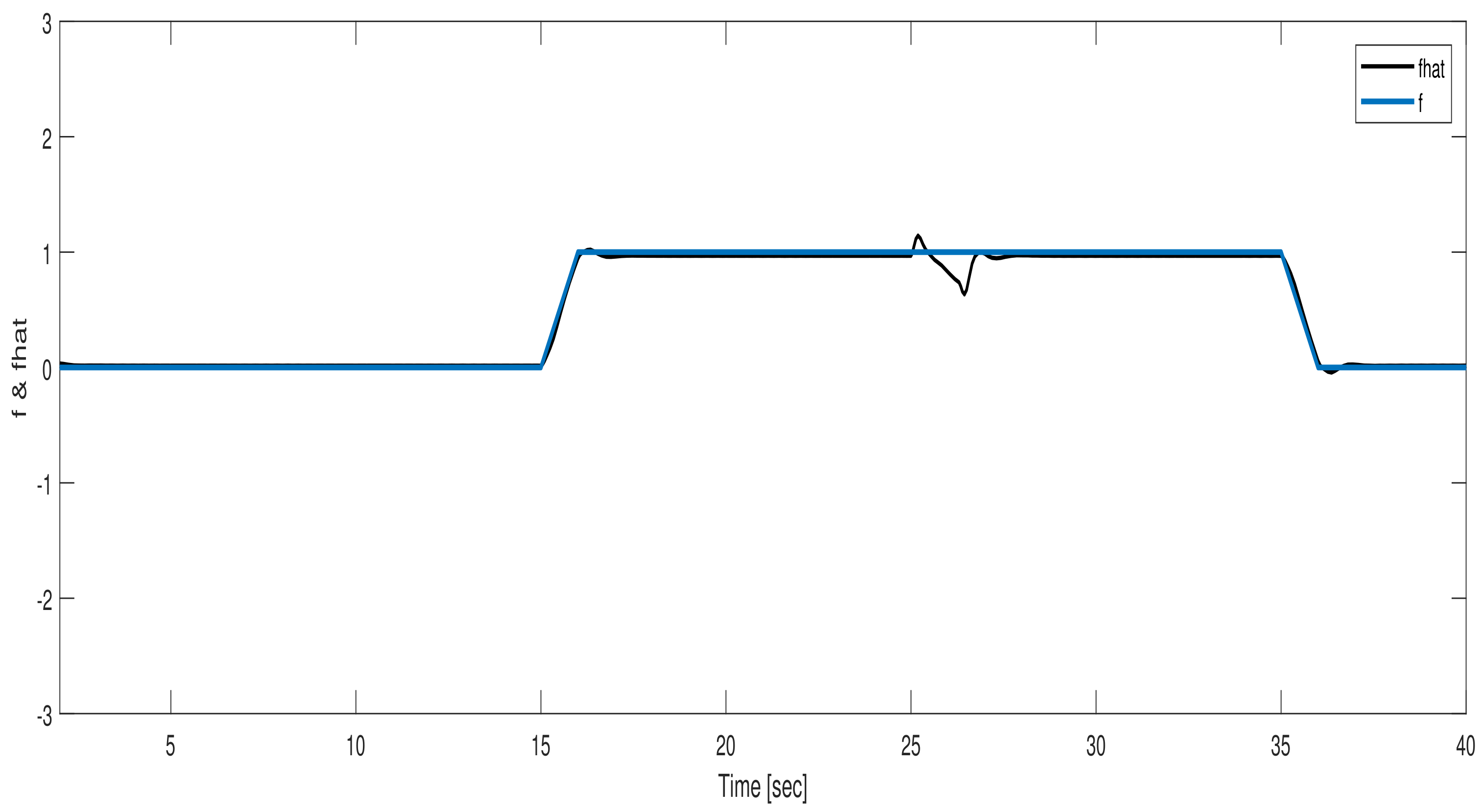
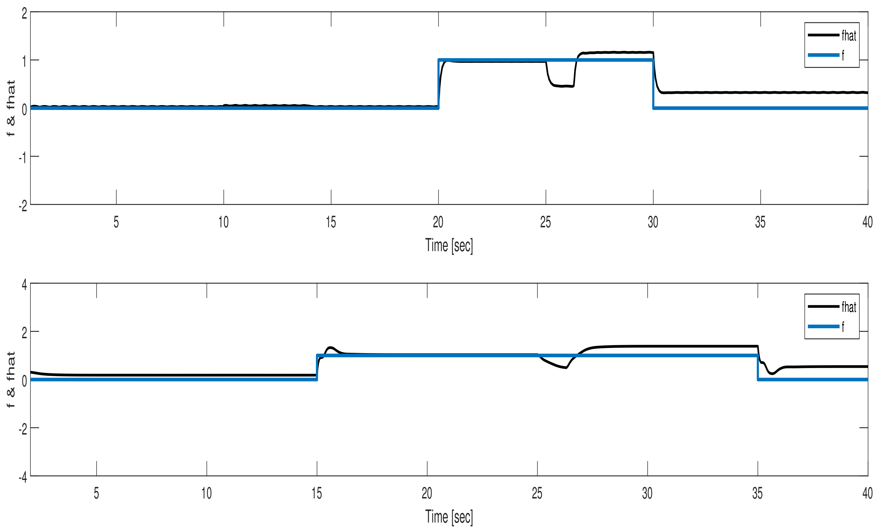
6.3. Simultaneous Actuator and Sensor Faults

First, using the transformation in (49), the system is decomposed as in (50) and (51). Then, using the results in Theorem 5, the LMIs (60) and (61) are solved, and the observer gains are obtained from (64) and (65):

$$\begin{array}{c}\hfill G_n=\left[\begin{array}{ccc}0.41& -0.43& -1.25\\ -0.27& 0.12& -0.16\\ -1.16& -0.24& -2.25\end{array}\right],G_l=\left[\begin{array}{ccc}8.87& -66.57& 2.22\\ 10.45& -0.6& 0.52\\ -2.45& 7.92& -0.52\end{array}\right].\end{array}$$

Finally, the simultaneous actuator and sensor faults are reconstructed using (69) and (74). In this case, the parameters are chosen as given in the previous part. Figure 6 and Figure 7 show the comparison of the simultaneous actuator and sensor fault reconstruction of the proposed method with [32] in the presence of $\partial (t,y,u)=\left[0.3,-0.5,0\right], y=0.3z_5-0.5z_6$, and $d\left(t\right)=u(t-20)$. The results verify that despite the existence of unknown disturbance and uncertainty, the proposed method performs well in the reconstruction of both sensor and actuator faults.

Considering the dynamics of disturbance in the sliding mode observer design, there was a reduced impact of disturbance in fault reconstruction in comparison with the approach presented in [32]. In other words, the proposed approach in Theorem 5 has the quick response in the fault reconstruction process when disturbance is entered to the system. In order to measure and investigate the performance of the proposed methods, it is required to use quantitative criteria. In

Table 1. The comparison of the norm specification of the simultaneous faults reconstruction.

	${∥\mathit{error}∥}_2\left(\mathit{Actuator}\right)$	${∥\mathit{error}∥}_2\left(\mathit{Sensor}\right)$
Theorem 5	29.04	99.07
[32]	32.61	103.87
Improvement (%)	10.9	4.6

, the norm specifications of the sensor and actuator fault detection errors for the proposed approach and the method represented in [32] are calculated. As can be seen in Table 1, the proposed approach improves the accuracy of the actuator fault reconstruction more than $10\%$ and the accuracy of the sensor fault reconstruction more than $4\%$.

7. Conclusions

In this paper, an efficient robust approach is proposed for simultaneous sensor and actuator faults reconstruction in the presence of both unknown disturbance and uncertainty. First, an SMO-based method was proposed, and the observer gains were derived utilizing an LMI-based method. Then, considering that the system is subject to both disturbance and uncertainty, a robust reconstruction method is proposed, and incorporating the concept of BRL, the fault reconstruction problem is represented as an LMI problem and solved using the available tools. Furthermore, utilizing a wind turbine system, the performance and robustness of the proposed method were demonstrated. The proposed method can be robust against of disturbances and uncertainties, which is the most important advantage of our work. In contrast, the reconstruction of the faults is under the bounded disturbance, which can be our work’s disadvantage. Finally, it is noted that although in many nonlinear systems, the nonlinearity and the effects of linearization error can be captured by the disturbances/uncertainties as considered in this paper, as an ongoing future work, it is quite beneficial to extend the proposed approach for pure nonlinear models in the presence of disturbances/uncertainties.

References

1. Saif, M.; Guan, Y. A new approach to robust fault detection and identification. IEEE Trans. Aerosp. Electron. Syst. 1993, 29, 685–695. [Google Scholar] [CrossRef]
2. Zhang, A.A.; Lv, B.C.; Zhang, C.Z.; She, D.Z. Finite time fault tolerant attitude control-based observer for a rigid satellite subject to thruster faults. IEEE Access 2017, 5, 16808–16817. [Google Scholar] [CrossRef]
3. Ghanbarpour, K.; Bayat, F.; Jalilvand, A. Wind turbines sustainable power generation subject to sensor faults: Observer-based MPC approach. Int. Trans. Electr. Energy Syst. 2020, 30, e12174. [Google Scholar] [CrossRef]
4. Taherkhani, A.; Bayat, F. Wind turbines robust fault reconstruction using adaptive sliding mode observer. IET Gener. Transm. Distrib. 2019, 13, 3096–3104. [Google Scholar] [CrossRef]
5. Yin, S.; Huang, Z. Performance monitoring for vehicle suspension system via fuzzy positivistic C-means clustering based on accelerometer measurements. IEEE/ASME Trans. Mechatron. 2014, 20, 2613–2620. [Google Scholar] [CrossRef]
6. Zhang, B.; Lu, S. Fault-tolerant control for four-wheel independent actuated electric vehicle using feedback linearization and cooperative game theory. Control Eng. Pract. 2020, 101, 104510. [Google Scholar] [CrossRef]
7. Sakthivel, R.; Selvaraj, P.; Mathiyalagan, K.; Park, J.H. Robust fault-tolerant Hinf control for offshore steel jacket platforms via sampled-data approach. J. Frankl. Inst. 2015, 352, 2259–2279. [Google Scholar] [CrossRef]
8. Gonzalez-Prieto, I.; Duran, M.J.; Rios-Garcia, N.; Barrero, F.; Martin, C. Open-switch fault detection in five-phase induction motor drives using model predictive control. IEEE Trans. Ind. Electron. 2017, 65, 3045–3055. [Google Scholar] [CrossRef]
9. Su, X.; Liu, X.; Song, Y.D. Fault-tolerant control of multiarea power systems via a sliding-mode observer technique. IEEE/ASME Trans. Mechatron. 2017, 23, 38–47. [Google Scholar] [CrossRef]
10. Ghanbarpour, K.; Bayat, F.; Jalilvand, A. Dependable power extraction in wind turbines using model predictive fault tolerant control. Int. J. Electr. Power Energy Syst. 2020, 118, 105802. [Google Scholar] [CrossRef]
11. Guzman, J.; Lopez-Estrada, F.R.; Estrada-Manzo, V.; Valencia-Palomo, G. Actuator fault estimation based on a proportional-integral observer with nonquadratic Lyapunov functions. Int. J. Syst. Sci. 2021, 52, 1938–1951. [Google Scholar] [CrossRef]
12. Tan, C.P.; Edwards, C. Sliding mode observers for robust detection and reconstruction of actuator and sensor faults. Int. J. Robust Nonlinear Control 2003, 13, 443–463. [Google Scholar] [CrossRef]
13. Sharma, R.; Aldeen, M. Fault detection in nonlinear systems with unknown inputs using sliding mode observer. In Proceedings of the 2007 American Control Conference, New York, NY, USA, 9–13 July 2007; pp. 432–437. [Google Scholar]
14. Rayankula, V.; Pathak, P.M. Fault Tolerant Control and Reconfiguration of Mobile Manipulator. J. Intell. Robot. Syst. 2021, 101, 1–18. [Google Scholar] [CrossRef]
15. Van Nguyen, T.; Ha, C. Experimental study of sensor fault-tolerant control for an electro-hydraulic actuator based on a robust nonlinear observer. Energies 2019, 12, 4337. [Google Scholar] [CrossRef] [Green Version]
16. Selvaraj, P.; Kaviarasan, B.; Sakthivel, R.; Karimi, H.R. Fault-tolerant SMC for Takagi–Sugeno fuzzy systems with time-varying delay and actuator saturation. IET Control. Theory Appl. 2017, 11, 1112–1123. [Google Scholar] [CrossRef]
17. Vaidyanathan, S.; Dolvis, L.G.; Jacques, K.; Lien, C.H.; Sambas, A. A new five-dimensional four-wing hyperchaotic system with hidden attractor, its electronic circuit realisation and synchronisation via integral sliding mode control. Int. J. Model. Identif. Control 2019, 32, 30–45. [Google Scholar] [CrossRef]
18. Mobayen, S.; Fekih, A.; Vaidyanathan, S.; Sambas, A. Chameleon Chaotic Systems With Quadratic Nonlinearities: An Adaptive Finite-Time Sliding Mode Control Approach and Circuit Simulation. IEEE Access 2021, 9, 64558–64573. [Google Scholar] [CrossRef]
19. Hou, Y.Y.; Fang, C.S.; Lien, C.H.; Vaidyanathan, S.; Sambas, A.; Mamat, M.; Johansyah, M.D. Rikitake dynamo system, its circuit simulation and chaotic synchronization via quasi-sliding mode control. Telkomnika 2021, 19, 1291–1301. [Google Scholar] [CrossRef]
20. Zhu, Q.; Li, Z.; Tan, X.; Xie, D.; Dai, W. Sensors fault diagnosis and active fault-tolerant control for PMSM drive systems based on a composite sliding mode observer. Energies 2019, 12, 1695. [Google Scholar] [CrossRef] [Green Version]
21. Yang, J.; Zhu, F. FDI design for uncertain nonlinear systems with both actuator and sensor faults. Asian J. Control. 2015, 17, 213–224. [Google Scholar] [CrossRef]
22. Taherkhani, A.; Bayat, F.; Mobayen, S.; Bartoszewicz, A. Dependable Sensor Fault Reconstruction in Air-Path System of Heavy-Duty Diesel Engines. Sensors 2021, 21, 7788. [Google Scholar] [CrossRef] [PubMed]
23. Zhang, X. Sensor bias fault detection and isolation in a class of nonlinear uncertain systems using adaptive estimation. IEEE Trans. Autom. Control 2011, 56, 1220–1226. [Google Scholar] [CrossRef]
24. Defoort, M.; Veluvolu, K.C.; Rath, J.J.; Djemai, M. Adaptive sensor and actuator fault estimation for a class of uncertain Lipschitz nonlinear systems. Int. J. Adapt. Control. Signal Process. 2016, 30, 271–283. [Google Scholar] [CrossRef]
25. You, F.; Li, H.; Wang, F.; Guan, S. Robust fast adaptive fault estimation for systems with time-varying interval delay. J. Frankl. Inst. 2015, 352, 5486–5513. [Google Scholar] [CrossRef]
26. Selvaraj, P.; Sakthivel, R.; Kwon, O.M. Synchronization of fractional-order complex dynamical network with random coupling delay, actuator faults and saturation. Nonlinear Dyn. 2018, 94, 3101–3116. [Google Scholar] [CrossRef]
27. Selvaraj, P.; Sakthivel, R.; Ahn, C.K. Observer-based synchronization of complex dynamical networks under actuator saturation and probabilistic faults. IEEE Trans. Syst. Man Cybern. Syst. 2018, 49, 1516–1526. [Google Scholar] [CrossRef]
28. Pinto, H.L.D.C.P.; Oliveira, T.R.; Hsu, L. Sliding mode observer for fault reconstruction of time-delay and sampled-output systems—A Time Shift Approach. Automatica 2019, 106, 390–400. [Google Scholar] [CrossRef]
29. Yang, C.; Liu, J.; Zeng, Y.; Xie, G. Real-time condition monitoring and fault detection of components based on machine-learning reconstruction model. Renew. Energy 2019, 133, 433–441. [Google Scholar] [CrossRef]
30. Harkat, M.F.; Mansouri, M.; Abodayeh, K.; Nounou, M.; Nounou, H. New sensor fault detection and isolation strategy–based interval-valued data. J. Chemom. 2020, 34, e3222. [Google Scholar] [CrossRef]
31. Lee, D.J.; Park, Y.; Park, Y.S. Robust H Sliding Mode Descriptor Observer for Fault and Output Disturbance Estimation of Uncertain Systems. IEEE Trans. Autom. Control 2012, 57, 2928–2934. [Google Scholar] [CrossRef]
32. Ben Brahim, A.; Dhahri, S.; Ben Hmida, F.; Sellami, A. Simultaneous actuator and sensor faults reconstruction based on robust sliding mode observer for a class of nonlinear systems. Asian J. Control 2017, 19, 362–371. [Google Scholar]
33. Brahim, A.B.; Dhahri, S.; Hmida, F.B.; Sellami, A. Simultaneous actuator and sensor faults estimation design for LPV systems using adaptive sliding mode observers. Int. J. Autom. Control 2021, 15, 1–27. [Google Scholar] [CrossRef]
34. You, G.; Xu, T.; Su, H.; Hou, X.; Li, J. Fault-tolerant control for actuator faults of wind energy conversion system. Energies 2019, 12, 2350. [Google Scholar] [CrossRef] [Green Version]
35. Tan, C.P.; Edwards, C. An LMI approach for designing sliding mode observers. Int. J. Control 2001, 74, 1559–1568. [Google Scholar] [CrossRef]
36. Alwi, H.; Edwards, C.; Tan, C.P. Fault Detection and Fault-Tolerant Control Using Sliding Modes; Springer Science & Business Media: Berlin/Heidelberg, Germany, 2011. [Google Scholar]
37. Bhat, S.P.; Bernstein, D.S. Finite-time stability of continuous autonomous systems. SIAM J. Control. Optim. 2000, 38, 751–766. [Google Scholar] [CrossRef]
38. Mahmoud, C.; Pascal, G. H design with pole placement constraints: An LMI approach. IEEE Trans. Autom. Control 1996, 41, 358–367. [Google Scholar]
Figure 1. Illustration of robust actuator fault reconstruction (fault on the first actuator).
Energies 15 01411 g001
Figure 2. Illustration of robust actuator fault reconstruction (fault on the second actuator).
Energies 15 01411 g002
Figure 3. Illustration of robust sensor fault reconstruction (pitch angle sensor fault).
Energies 15 01411 g003
Figure 4. Illustration of robust sensor fault reconstruction (rotor speed sensor fault).
Energies 15 01411 g004
Figure 5. Illustration of robust sensor fault reconstruction (generator speed sensor fault).
Energies 15 01411 g005
Figure 6. The simultaneous actuator and sensor fault reconstruction using the approach proposed in Theorem 5.
Energies 15 01411 g006
Figure 7. The simultaneous actuator and sensor fault reconstruction using the approach presented in [32].
Energies 15 01411 g007