Article

Dynamic Price-Based Demand Response through Linear Regression for Microgrids with Renewable Energy Resources

1
Department of Electrical Engineering, The University of Faisalabad, Faisalabad 38000, Pakistan
2
Department of CS & IT, University of Kotli, Azad Jammu & Kashmir, Azad Jammu and Kashmir 11100, Pakistan
3
School of Computer Science, Neijiang Normal University, Neijiang 641100, China
4
College of Physics and Electronic Information Engineering, Neijiang Normal University, Neijiang 641100, China
5
Faculty of Economics and Business, University of Debrecen, 4032 Debrecen, Hungary
6
College of Business and Economics, University of Johannesburg, Johannesburg 2006, South Africa
7
Hungarian National Bank—Research Center, John von Neumann University, Izsáki út 10, 6000 Kecskemét, Hungary
*
Author to whom correspondence should be addressed.
Energies 2022, 15(4), 1385; https://doi.org/10.3390/en15041385
Submission received: 31 December 2021 / Revised: 2 February 2022 / Accepted: 8 February 2022 / Published: 14 February 2022
(This article belongs to the Special Issue Technology Management and Innovation in the Energy Field)

Abstract

:
The green innovations in the energy sector are smart solutions to meet the excessive power requirements through renewable energy resources (RERs). These resources have forwarded the revolutionary relief in control of carbon dioxide gaseous emissions from traditional energy resources. The use of RERs in a heuristic manner is necessary to meet the demand side management in microgrids (MGs). The pricing scheme limitations hinder the profit maximization of MG and their customers. In addition, recent pricing schemes lack mechanistic underpinning. Therefore, a dynamic electricity pricing scheme through linear regression is designed for RERs to maximize the profit of load customers (changeable and unchangeable) in MG. The demand response optimization problem is solved through the particle swarm optimization (PSO) technique. The proposed dynamic electricity pricing scheme is evaluated under two different scenarios. The simulation results verified that the proposed dynamic electricity pricing scheme sustained the profit margins and comforts for changeable and unchangeable load customers as compared to fixed electricity pricing schemes in both scenarios. Hence, the proposed dynamic electricity pricing scheme can readily be used for real microgrids (MGs) to grasp the goal for cleaner energy production.

1. Introduction

The high energy demand has not only resulted in shortage of input reserves but also has increased the air pollution through gaseous emission. Hence, the production of pollution-free energy is a global concern which needs to be solved on an urgent basis. In this scenario, a smartgrid (SG) is introduced that can generate energy in reliable and efficient way at a low cost [1]. Moreover, the efficiency of the SG is further enhanced through the development of a microgrid (MG) in it [2,3].
The demand management for customers is the only linkage available to solve energy production problems and also aid in conservation of input resources. For this purpose, the demand side management (DSM) technique is presented. In addition to energy conservation, this technique has increased the lifespan and reliability of power grids along with satisfaction of load demand, and also gaseous emission is decreased [4]. The DSM is sub-classified into the following programs: conservation and energy efficiency, and demand response (DR) [5].
Basically, DR is a vital component of SG which interrelates utilities and system operators by providing real-time updates to the electricity infrastructure for the replacement of traditional resources with intermittent ones (such as solar and wind energy) which eventually results in cost reduction, and also ensures the customers can reduce their electricity bills [6,7]. Various aspects comprising (a) offered motivations/incentives, (b) decision variables/parameters, and (c) control mechanisms/techniques have been used to classify DR programs [8,9]. The offered motivations/incentives are sub-categorized into incentive-based and price/time-based schemes. Both schemes offer some incentives to customers based on their load reduction. Three factors, i.e., real-time pricing (RTP), time of use (TOU) pricing, and critical peak (CPP) pricing, regulate the price of electricity in price-based DR [10]. In the case of incentive-based DR, electricity prices may or may not be flexible, depending upon direct load control programs, demand bidding programs, emergency DR programs, interruptible/curtailable rates (I/C) and capacity market programs [11]. The category (b) of DR schemes is classified into task scheduling and energy management [12]. The usage of energy according to peak demand hours is defined as energy management DR. The control techniques (c) are further sub-classified as centralized and decentralized modes [13]. Both modes differ based on users’ interface interaction, i.e., direct and indirect with utility for load consumption.
In the literature, a number of researchers [14,15,16,17,18,19,20,21] have used DR on industrial and residential scales. At industrial level, Xu et al. [14] stated that industries are categorized into different groups via utility depending upon DR potential. Moreover, each individual group have specific pricing schemes based on optimum load features. In contrast, energy management is used as a tool for implication of DR at the residential scale. Ref. [17] used DR price in real time that was optimized through stochastic and robust scheme for residential appliances. The smart meter integrated with this scheme (also considered uncertainties) could automatically convey the message to users so that they can optimize their electricity accordingly within 5 min of the timespan. The lack of pricing signal design was observed in this study. In another write-up, Yi et al. [21] scheduled the appliances in real time at small residential DR by using an optimal stopping scheme. In this scheme, the various equipment are grouped and used according to predefined time (principled on two-stage scheduling algorithm), and it eventually results in bill-saving. The aim of [22,23,24] was to reduce the electricity bills by keeping the consumer’s comfort at a higher priority. For this purpose, they used multidisciplinary optimization approaches. The bilevel programming in DR was utilized by [25] to attain marginal prices through unit commitment (upper level) and to reduce the overall operational cost (lower level).
Ref. [26] introduced the bilevel programming, in which numerous microgrids (MGs) are integrated to investigate the interaction between a large central production unit and an energy service provider (ESP). This stepwise process is carried out in the following manner: (a) the central production unit is used for formation and optimization of energy price, (b) the price signals are sent to EPS after price optimization, and (c) the energy received from central production is further optimized by EPS which schedules the energy generation consumption. The lack of interaction between utility grid and renewable energy resources (RERs) was analyzed in this work. Ref. [27] introduced time- or price-based self-scheduling models in the day-ahead energy markets to increase the profit of DR aggregators. This model was based on mixed-integer linear programming (MILP). The DR was subjected to various procurement methods such as load shifting and load curtailment, and consumption of in situ (onsite) generation and energy storage systems (ESSs) for small to medium sized users. The DR aggregator has some problems related to wholesale market operations due to its direct interface with the wholesale market. Therefore, significant updates are required in the DR aggregator with respect to the wholesale market to integration of DR bids. Later on, a risk-aware stochastic optimization model was proposed by [28] to ensure profit increment of MG aggregator and, also, the interaction with electricity customers. In this model, the problem existed in the DR price that was fixed instead of dynamic and dependent upon the real operational conditions. The practical integration of DR in distribution networks based on optimal and pricing model was proposed by [29]. In bilevel programming, a leader (load serving entity (LSE)) and a follower (DR aggregator) are presented to develop an interaction between users and their LSE. The strong duality theorem and Karush–Kuhn–Tucker (KKT) conditions were used to transformed a nonlinear bilevel mixed-integer program into a single MILP. The changeable load customers experienced problems related to the wholesale price which was changed on an hourly basis. For leader and follower, a win–win solution was proposed for this scheme. This presented scheme was fruitful for both follower (payoff) and leader (profit). The uncertainties related to renewable resources were not focused on. In another work, the profit of utility was enhanced by manipulation of prices based on mean power consumption in a multi-agent environment [17,30]. The uncertainties of RERs were mentioned but not considered in their work. Figure 1 shows the idea of the paper.
The above discussion has shown that DR technique has been studied without proper description in literature [17,31,32,33,34], or only fixed electricity pricing schemes have been used [28,35]. As an example, throughout energy usage, the unchangeable load users have higher but constant proportion of profit as compared to changeable load users in fixed electricty pricing schemes. In the case of the RTP scheme, the pricing signal design has some constraints in term of design—either it was not mentioned or design was ambiguous—and also had negative influence on changeable load customers operating at small scales [17]. Keeping these facts in view, the present study aims to solve the above mentioned problems, and novel features are mentioned below:
  • The MG including photovoltaics (PVs) and wind turbines (WTs) is modeled in MATLAB/Simulink for two types of load customers (changeable and unchangeable).
  • The dynamic electricity pricing scheme is designed based on linear regression.
  • The optimization of the DR problem is solved through the particle swarm optimization (PSO) technique.
  • The profit is enhanced for changeable and unchangeable load customers.
  • The proposed scheme is favorable for small-scale changeable loads.
  • The proposed scheme has plug and play feature for a real world market.
The paper is summarized in the following manner: a novel dynamic electricty pricing scheme is modeled in Section 2. The technical constraints and objective functions are explained in Section 3. Section 4 introduces the system setup of grid-connected MG, while Section 5 and Section 6 contain numerical results and conclusions.

2. Dynamic Pricing Model

To overcome the greenhouse effects due to carbon dioxide gaseous emissions into the atmosphere, RERs play a leading role in production of economical clean energy to meet increased energy requirements. The RERs energy production is nonlinear in nature. The energy resources comprise PVs, WTs, and tidal power as recognized among other natural resources. The generation of these resources is integrated with main grid generation to encounter the demand of power in a power system. This is also the concept of MG, in which the power equation of a power system is maintained automatically. Figure 2 shows a grid-connected MG.
In an MG, the relationship between demand and supply is dynamic. Many researchers have investigated this relationship to improve the energy efficiency of MG through DSM. From literature survey, it can be concluded that optimized DR is considered to be beneficial for DSM, which will eventually enhance the efficiency of MG. The DR can reduce peaking plant and auxiliary services in an MG. However, there is a risk of overestimated modeling of the DR problem due to unrealistic assumptions about customers load utilization and RERs [36]. The DR modeling can be carried out by using two types of pricing schemes. One is time-based rate, the second is incentive-based rate [5]. In the time-based rate program, a dynamic electricity pricing scheme is preferred due to its high profits for changeable load customers [37]. In order to describe the employed dynamic electricity pricing scheme for the optimization of DR in MG, one should have knowledge of demand–price elasticity (DPE). The DPE signifies the relation between an increase in demand with a decrease in price, though the change in demand is dynamic. Therefore, linear regression is used to quantify the preceding change in demand. Through regression, the nonlinear demand curve can be linearized. Regression is a documented technique for load estimation [38]. Therefore, the designed dynamic electricity pricing scheme is favorable in terms of comfort for unchangeable load customers, whereas changeable load customers gain both decent profit and comfort. The dynamic electricity pricing scheme is given below:
y ( t ) = 1 0 i m 0 < j < n ( ( R N ) j ) i + D ( t ) P T ( t ) × ( d o p o )
where y ( t ) is the computed dynamic electricty price and R N represents active distributor generators (WT and PV) in the MG. The i represents the respective distributed generator (DG) being considered from active distributed generators (DGs) and can range up to m, j can range up to n, it represents specific renewable energy resource (RER) inside each DG. In this way, estimation parameters can be computed for the pricing signal, and the generation constraint can be rectified. The real-time power generation for load customers from RERs is represented by D(t). The total available power at time t is given by P T ( t ) . The parameter estimation for the random variable of demand is represented by the difference of initial values of demand d o and price p o , respectively.

3. Demand Response Model

3.1. Objective Function

The present study aimed at profit maximization of load customers by utilizing novel dynamic electricity pricing model which is as follows:
m a x   p r o f i t   o f   c u s t o m e r s = U x ( t ) y ( t ) × ( l i n f + l f ( t ) )
where U x ( t ) and l f ( t ) are the utility function and changeable load during time t, while l i n f is the unchangeable load. Basically, utility function is the total satisfaction of the user’s comfort in the sense of power utilization at a reasonable price. With respect to this definition, it is assumed that the user’s utility will have the following key points [39]:
  • Non-decreasing utility function should be used because it can fulfill the maximum desires of consumers.
  • The usage of first unit of electricity (accounted as satisfaction level/utility of consumers) should exceed the utility until the nth unit. At this moment, the user’s utility increased smoothly.
  • The zero-power utilization should result in zero utility.
Finally, it is found that objective function (utility) should have quadratic association with linear decreasing marginal profit [39,40]. The objective/utility function is as follows:
U x ( t ) = q x r x 2         0 x x m a x
where x represents the utilization of power by individual customers during time t, while the behavior of individual users in DR is subjected to their definition of utilization and is represented by parameters q and r, respectively.

3.2. Technical Constraints
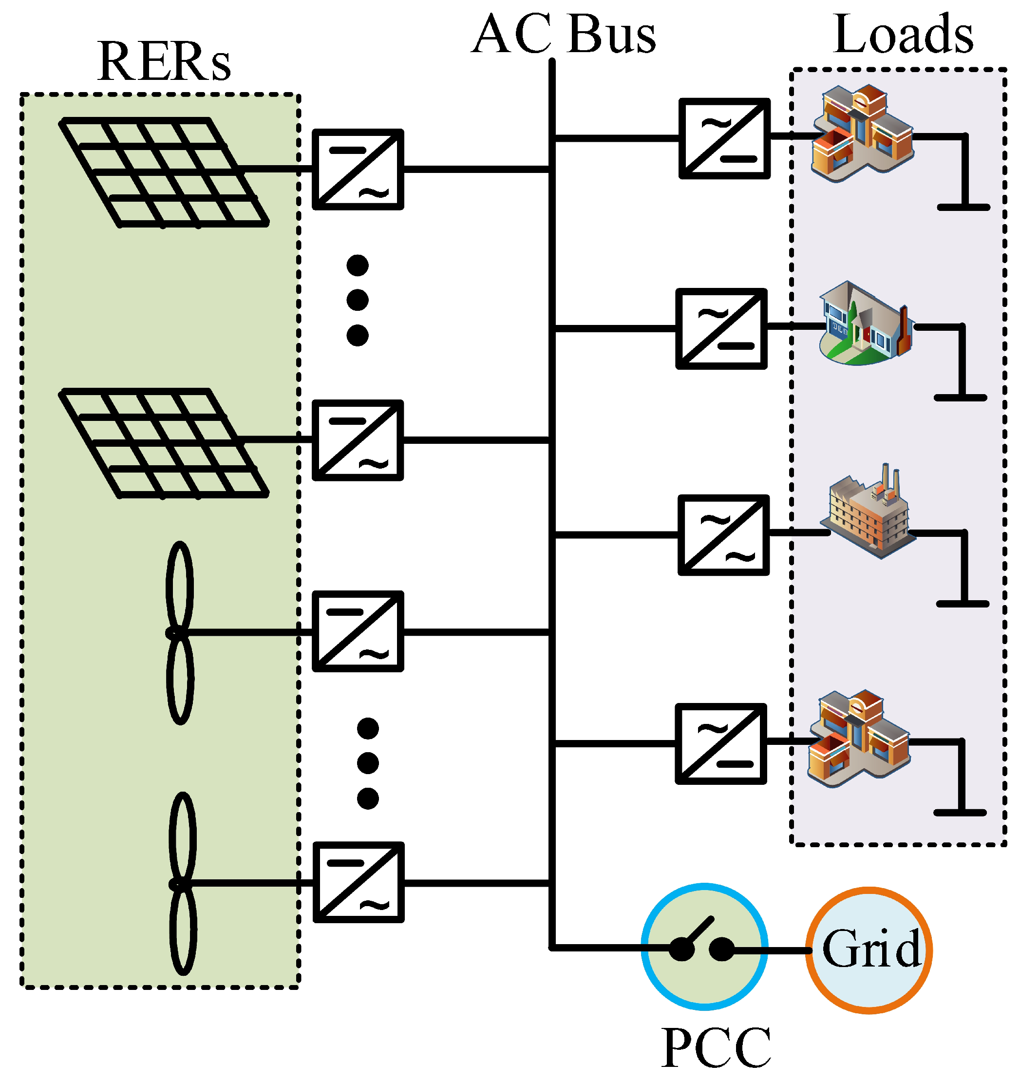
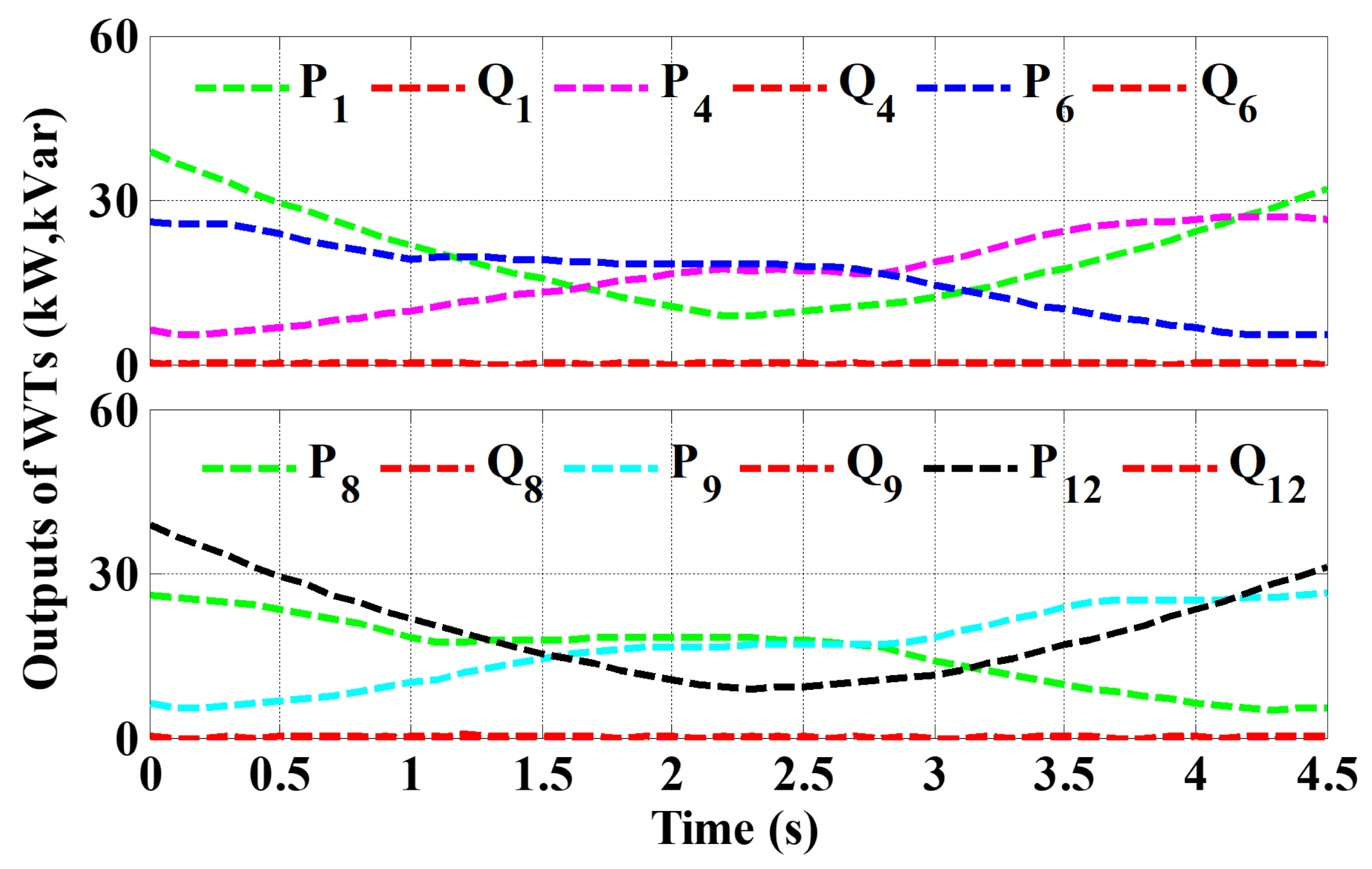
The objective function is solved through three constraints, i.e., equality (power balance) and inequality (generation and load limit), which are given below:
P T ( t ) + D ( t ) = l i n f + l f ( t )
P T m i n ( t ) P T ( t ) P T m a x ( t )
l f m i n ( t ) l f ( t ) l f m a x ( t )

4. System Setups

MATLAB/Simulink is used to design the grid-connected MG. The ( ( R N ) j ) i corresponds to DGs. The changeable loads fall in l o a d 1 to l o a d 5 and unchangeable in l o a d 6 to l o a d 1 2 . The DGs related to PVs are D G 2 , D G 3 , D G 5 , D G 7 , D G 10 , and D G 11 , while D G 1 , D G 4 , D G 6 , D G 8 , D G 9 , and D G 12 are WTs. The maximum power point tracking (MPPT) control mode is used to run PVs and WTs. The initial demand and supply define the numeric value for parameter estimation for random variable of demand. Table 1 (case I) and Table 2 (case II) represent the parameters of DGs and loads.

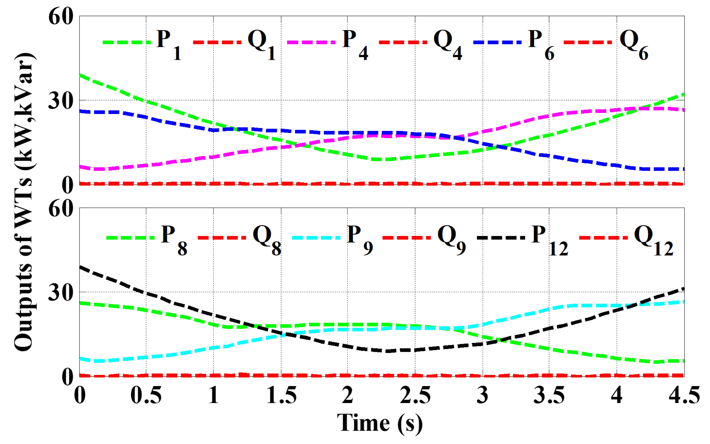
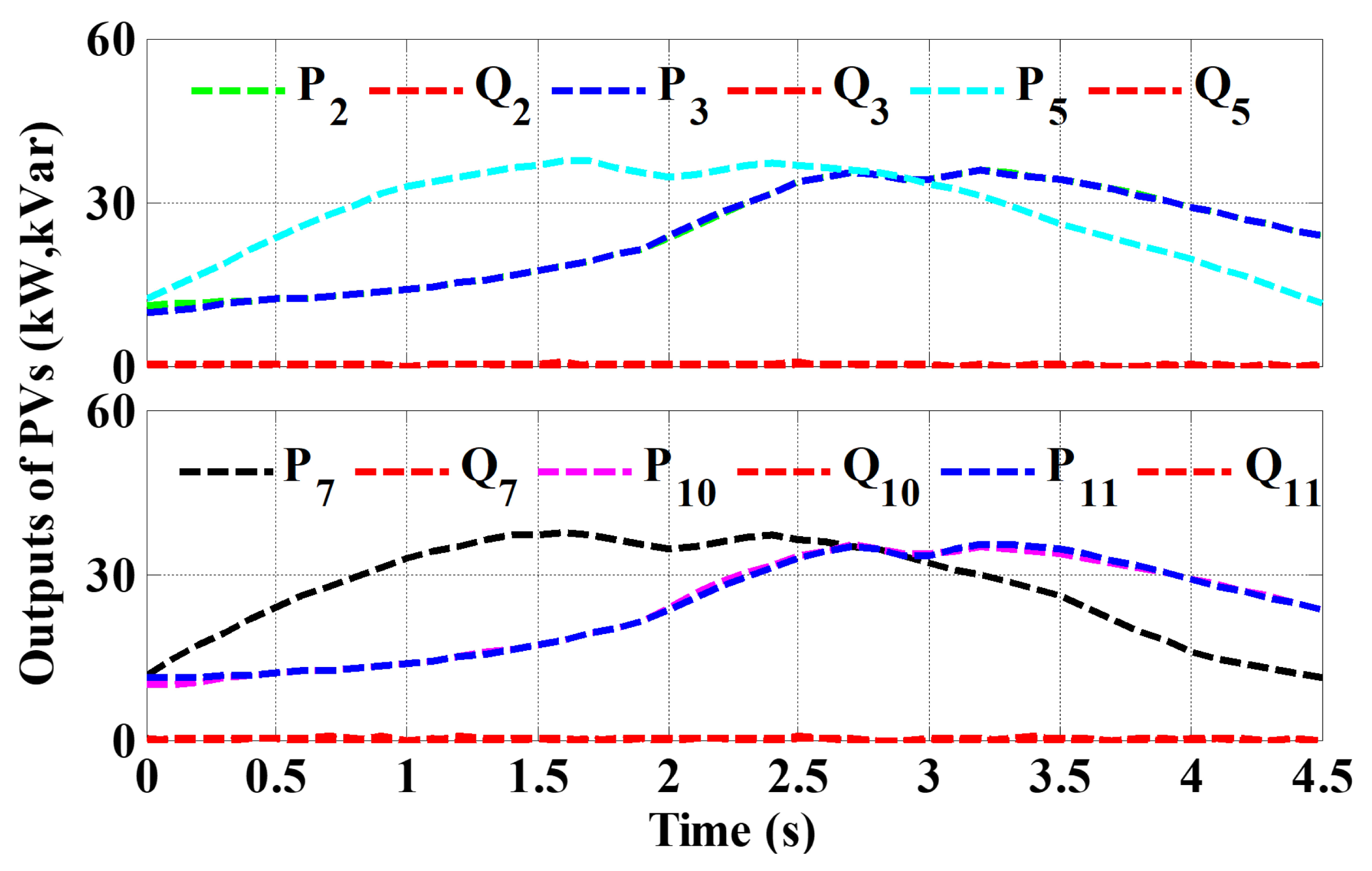
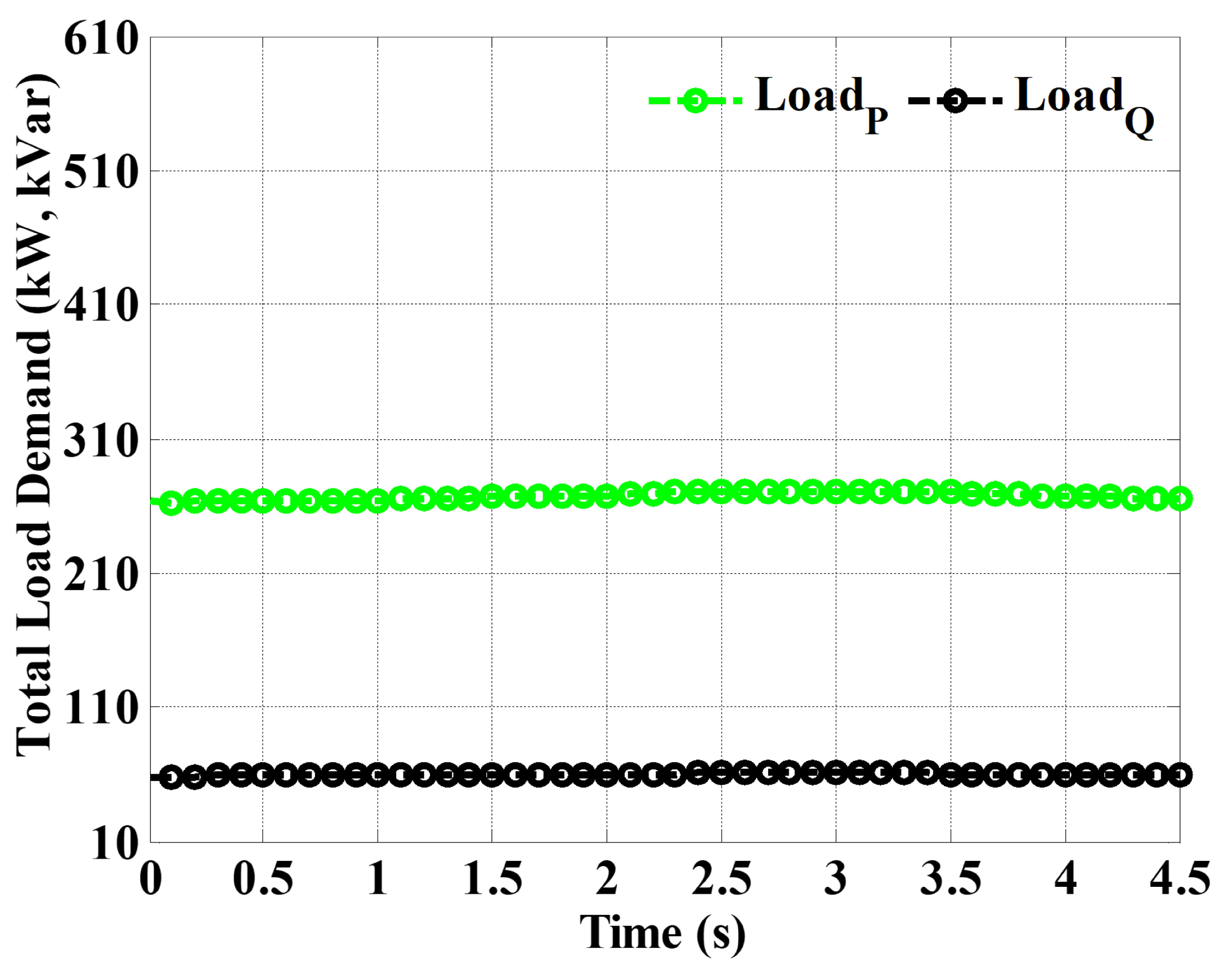
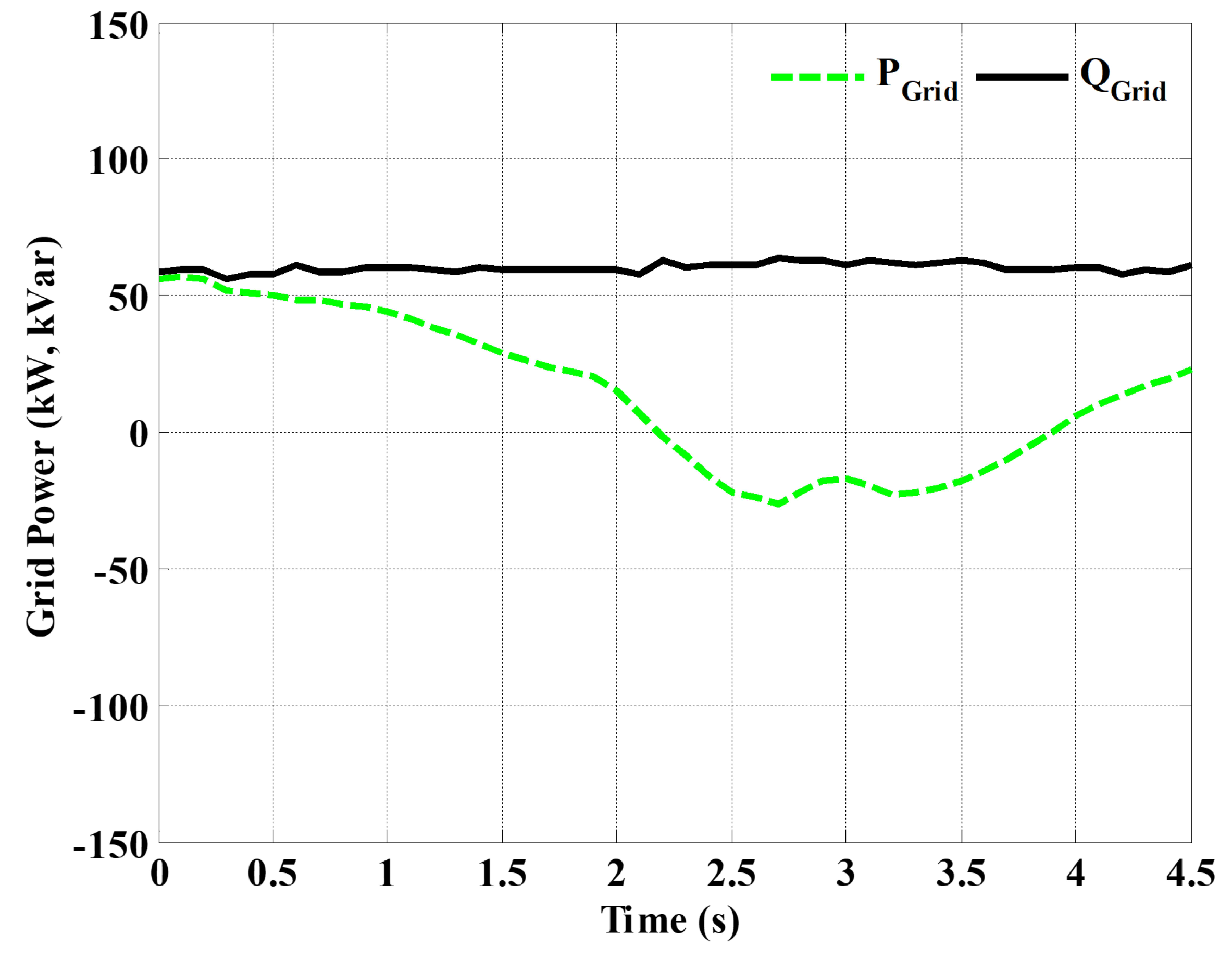
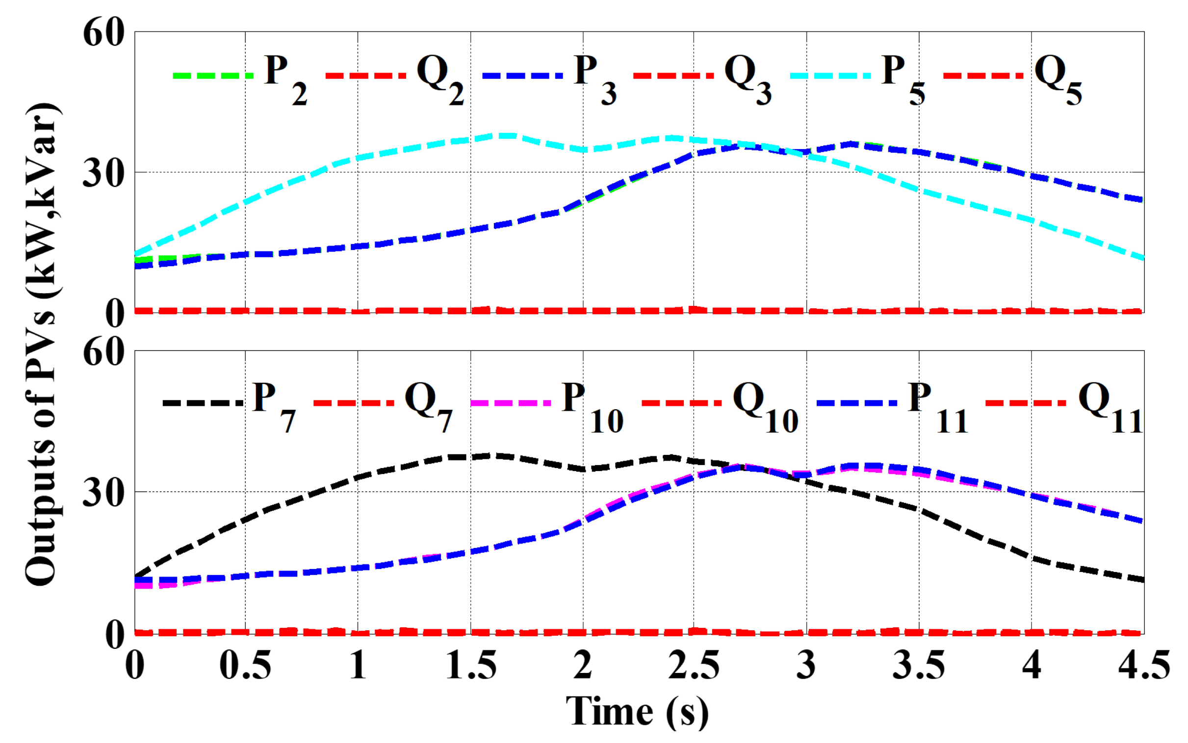
5. Results and Discussions

Two aspects are covered in this study to evaluate the efficiency of the proposed model by comparing with fixed electricity pricing scheme. The first aspect (case I) covers the implementation of dynamic electricity pricing scheme in MG for unchangeable power load. Regarding the second aspect (case II), both power load customers, i.e., changeable and unhangeable, are studied with respect to fixed and dynamic electricity pricing schemes.

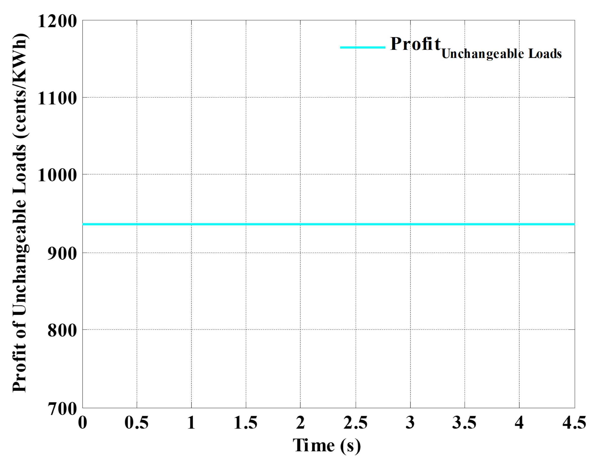
5.1. Case I: Comparison of Dynamic and Fixed Electricity Pricing Schemes for Unchangeable Loads

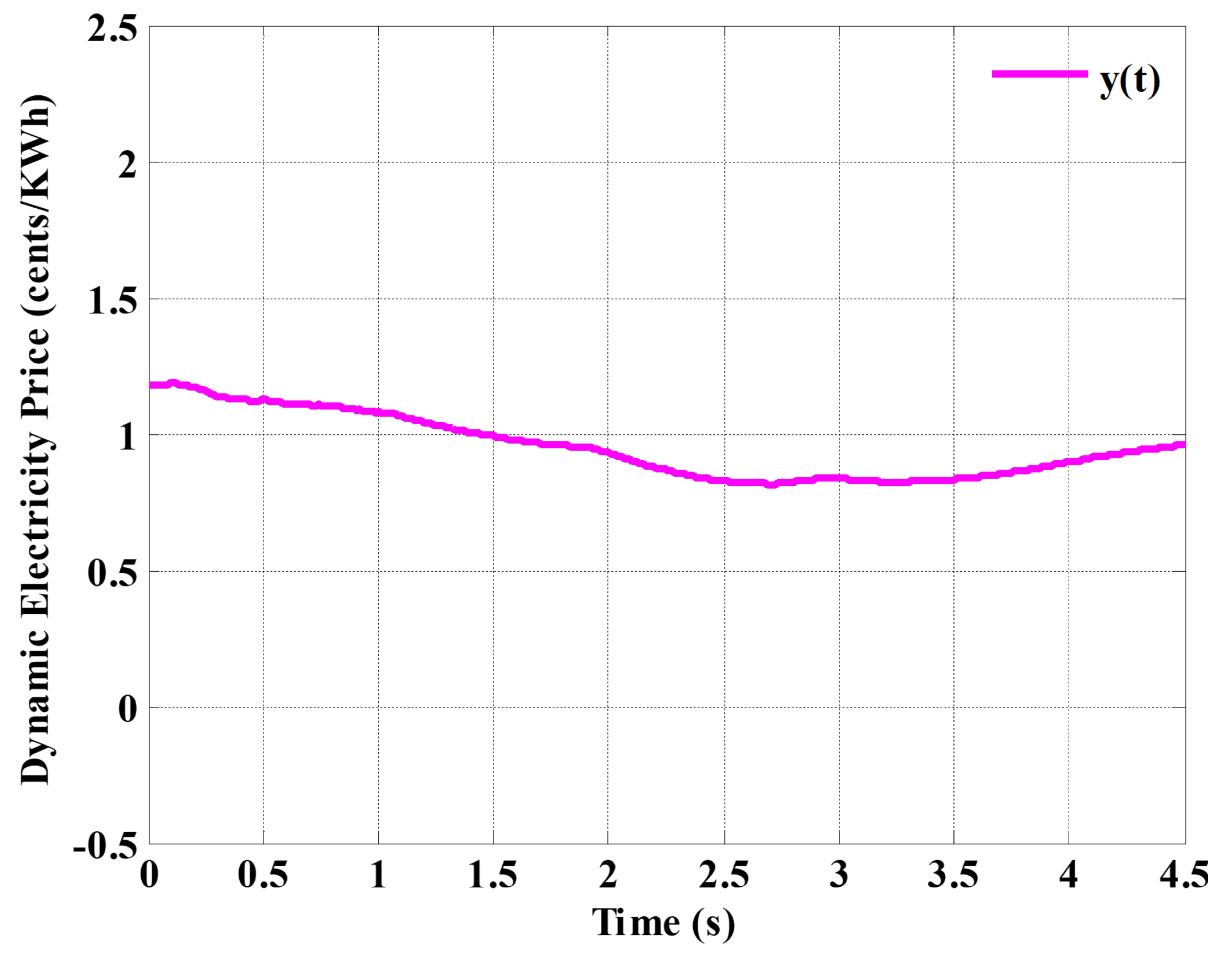
5.1.1. Dynamic Electricity Pricing Scheme

Figure 3 and Figure 4 show the active and reactive power outputs of WTs and PVs. The reactive power outputs are zero in both WTs and PVs. The randomness of natural resources (sunlight and wind speed) have influence on active power outputs of PVs ( D G 2 , D G 3 , D G 5 , D G 7 , D G 10 , and D G 11 ) and WTs ( D G 1 , D G 4 , D G 6 , D G 8 , D G 9 , and D G 12 ). With the passage of time, the gradual increment in active power outputs of D G 4 and D G 9 could be analyzed and its peak value is recorded at t = 4.5 s. In addition, similar trends regarding active power outputs are observed in the case of D G 1 and D G 12 with maximum value at time interval of four and half seconds (t = 4.5 s), while the active power outputs decreased with the passage of time in D G 6 and D G 8 , and minimum value is observed at t = 4.5 s. The maximum active power output at t = 2.5 s is observed in D G 5 and D G 7 in the case of PVs, and the remaining DGs ( D G 2 , D G 3 , D G 10 , and D G 11 ) have maximum active power output at same time interval (t = 2.5 s). The power output, either active or reactive, of the main grid is shown in Figure 5. The deficit caused by RERs is overcome by the main grid. In addition, excessive energy or active power output resulting from RERs is fed to the main grid.
The frequency and line voltages in MG can fluctuate due to natural environmental conditions and loads. In spite of severe variations in environmental conditions, the constant voltage of 380 V and frequency of 50 Hz is observed throughout the line during different loads (Figure 6). The total demand of unchangeable loads (1-12) is demonstrated in Figure 7. These figures show that load demand of users is in accordance with their satisfaction level. In a dynamic electricity pricing scheme, the variations in profit of unchangeable load clients are analyzed due to price variation in different time durations. This dynamic electricity pricing scheme is more profitable as compared to the fixed electricity pricing scheme used by [29] for unchangeable load users. Moreover, small- to medium-scale customers are considered in their work. The use of a dynamic electricity pricing scheme in previous study [41] was limited to small-scale unchangeable load customers, while the current study is suitable and profitable for a wide range (small–large scales) of customers in the distribution network. The dynamic electricity price is presented in Figure 8, and profit of unchangeable load is shown in Figure 9. Furthermore, profit of the unchangeable load customers starts from 5450 cents, and the maximum (5662 cents) is observed at time t = 2.7 s due to low dynamic electricity price. Conclusively, it is found that the present dynamic electricity pricing model is more profitable for unchangeable load customers as compared to the previous model [37].

5.1.2. Fixed Electricity Pricing Scheme

Figure 10 shows the profit of unchangeable load customers at 10 cents of the fixed electricity pricing scheme. The 943-cent profit is observed throughout the duration in the fixed electricity pricing scheme. However, the profit of the dynamic electricity pricing model is much higher than the fixed electricity pricing model, as verified by the results. Conclusively, it is found that the comfort and profit of unchangeable load customers are well maintained with the passage of time through the dynamic electricity pricing model as compared to the fixed electricity pricing model. Figure 11 describes the behavior of active and reactive power outputs of the main grid. At t = 0~2.2 s, the main grid supplies the active power outputs to the MG to entertain their loads due to lower outputs of RERs. Furthermore, the main grid absorbs the excessive output power by RERs after t = 2.2~4.5 s. The 60 kW reactive power load is supplied by the main grid.

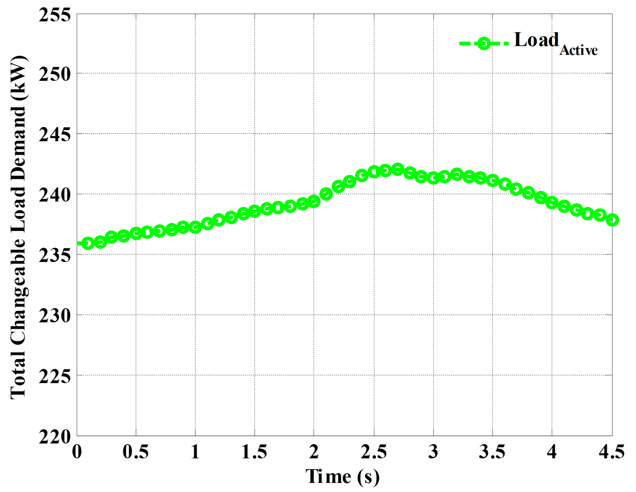
5.2. Case II: Comparison of Dynamic and Fixed Electricity Pricing Schemes-Based DR for Changeable and Unchangeable Loads

Both pricing schemes (dynamic and fixed electricity pricing schemes) are implemented in case II for unchangeable and changeable loads. The profit of changeable and comfort of unchangeable loads are compared with the fixed electricity pricing scheme.

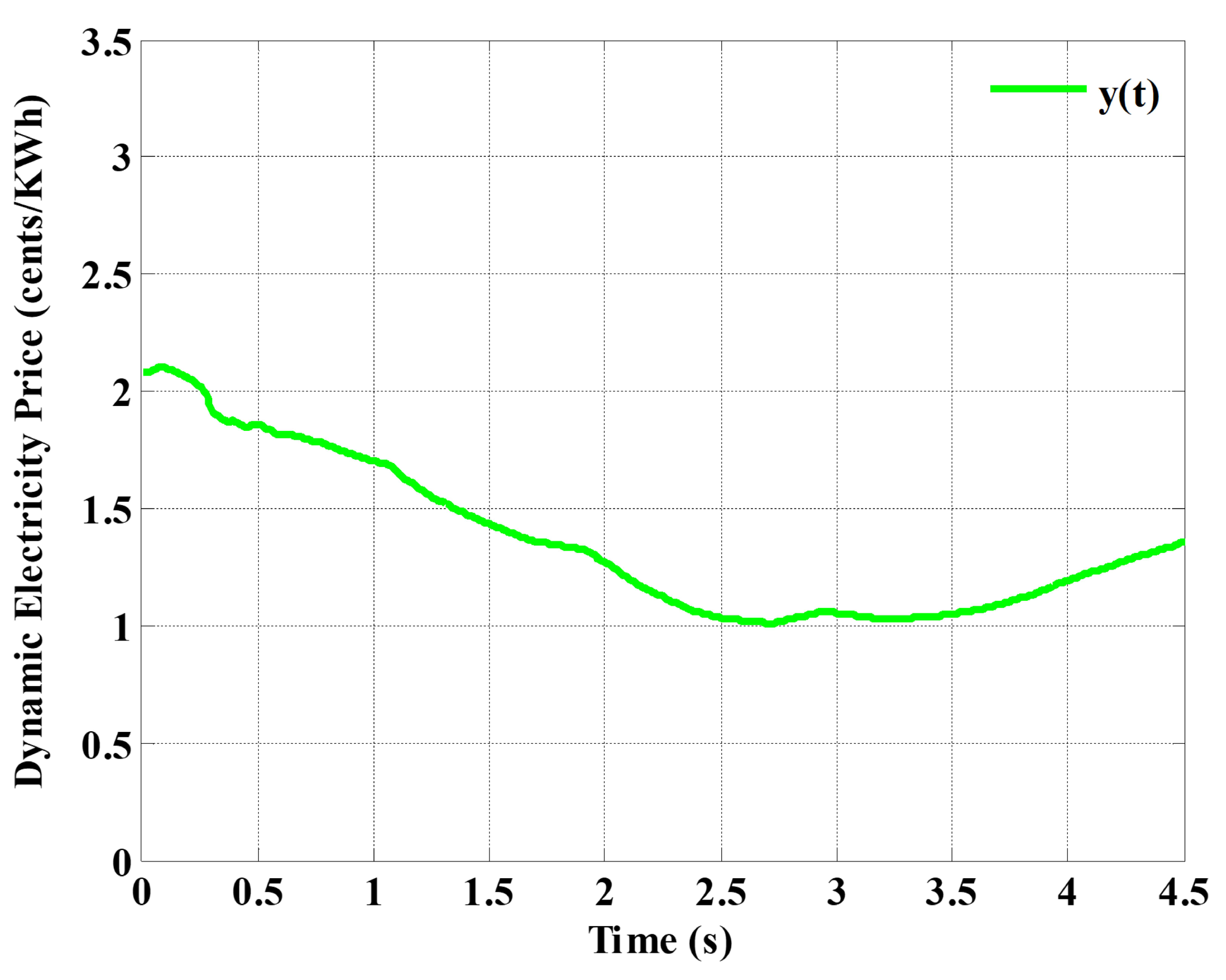
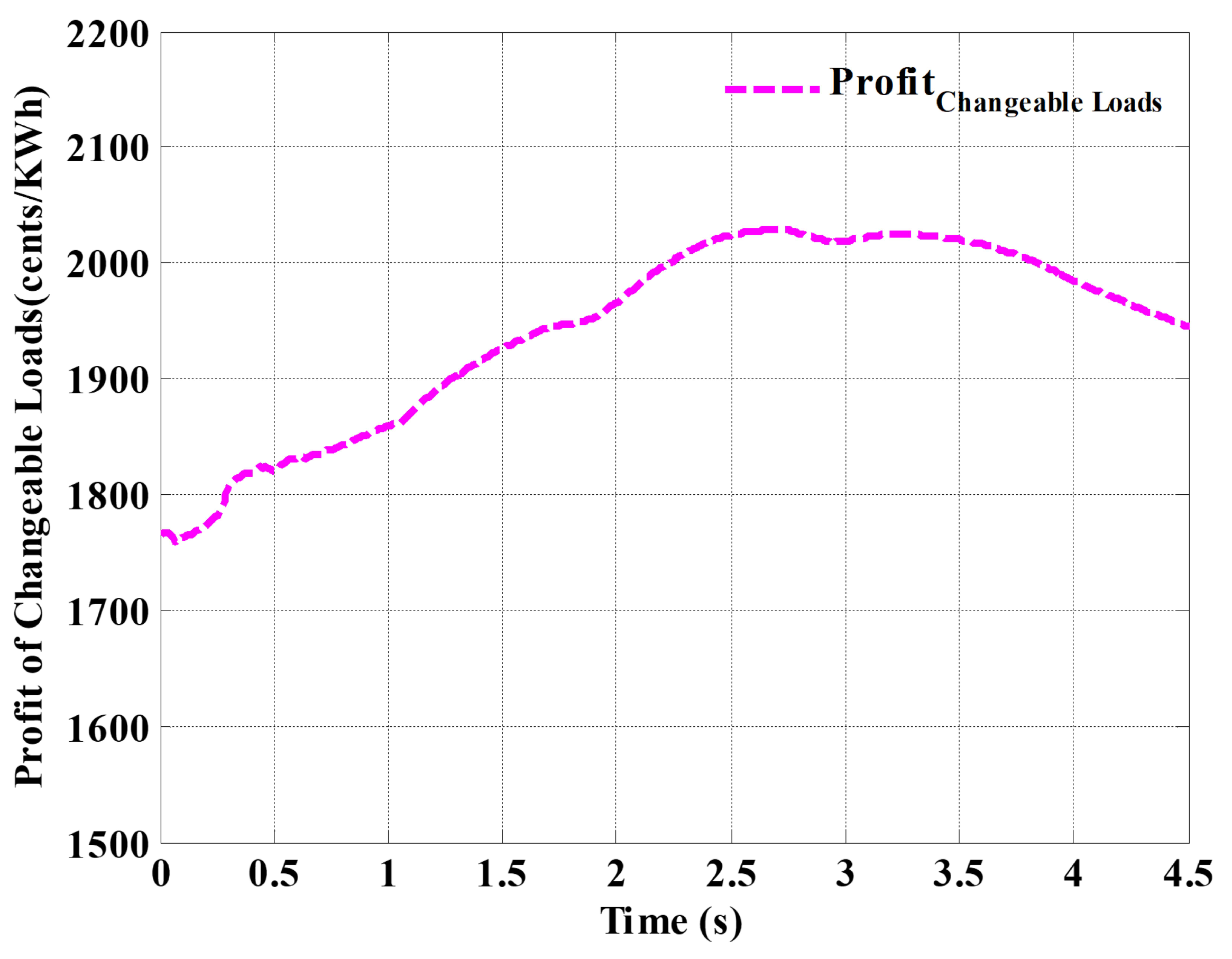
5.2.1. Dynamic Electricity Pricing Scheme

The reactive power of uncontrollable DGs comprising PVs and WTs are zero and can be seen in Figure 12 and Figure 13. The D G 1 , D G 4 , D G 6 , D G 8 , D G 9 , and D G 12 are WTs. The active power outputs of D G 4 and D G 9 are increasing, and D G 6 and D G 8 are decreasing, which can be seen from the figures. The WTs active power outputs depend upon the speed of wind. Moreover, at t = 4.5 s, the peak ( D G 4 and D G 9 ) and off-peak ( D G 6 and D G 8 ) active power outputs are noticed. However, D G 4 and D G 9 follow the same pattern as D G 1 and D G 12 , but at t = 4.5 s, the peak of active power outputs is observed. In the case of PVs, two patterns of active power outputs are observed: D G 5 and D G 7 are analogous, and D G 2 , D G 3 , D G 10 , and D G 11 are alike. The maximum active power outputs of D G 5 and D G 7 are analyzed at t = 2.5 s. In addition, D G 2 , D G 3 , D G 10 , and D G 11 have maximum active power outputs, which can be seen from Figure 13 at t = 2.5 s.
The output of main grid (active and reactive power output) can be seen from Figure 14. The load demand of customers varies with pricing model, which has a direct relation with RERs. In the case of lower outputs of RERs, the main grid facilitates MG and their customers and vice versa. At t = 0~4.5 s, the main grid supplied its active and reactive (70 kW) power outputs to load customers due to lower dynamic electricity price, which can be seen from Figure 14.
Figure 15 is representing the total demand of changeable loads. The changeable loads obtain the maximum profit (2029 cents at t = 3.2 s) due to lower dynamic electricity price (Figure 16), as verified by Figure 17. The comfort of changeable load customers might be disturbed under a fixed electricity pricing scheme [28]. In contrast, small-scale changeable load customers were charged through a dynamic electricity pricing scheme but the outcomes may not be favorable to large-scale changeable load customers as verified by [17,41,42]. Ref. [37] used the dynamic electricity pricing model based on RERs, and the maximum profit (1325 cents) of changeable load customers is observed at t = 2.2 s. However, the present dynamic electricity pricing model based on regression analysis is more beneficial for changeable and unchangeable load customers at small and large scales. In addition, the comfort for unchangeable load customers is maintained throughout the case.

5.2.2. Fixed Electricity Pricing Scheme

The profit of changeable load customers (213 cents) at the fixed (10 cents) electricity pricing scheme can be seen from Figure 18. As per the fixed electricity pricing scheme, load demand is price-oriented by a higher price lowering the load demand. Simply, changeable load customers reduce their load demand due to high regular price and vice versa (dynamic electricity pricing scheme). The reduction in load demand by changeable load customers resulted in lower profit. Hence, the fixed electricity pricing scheme is proven to be uncomfortable for changeable load customers. According to Figure 19, it can be seen that main grid active power output is fed into MG for their customers from t = 0~2 s. From t = 2~4.2 s, the main grid absorbs the excessive output power of RERs due to the fixed electricity pricing scheme.

6. Conclusions

The maximization of profit for changeable and unchangeable load customers is objectively aimed for optimization of DR in MG through the dynamic electricity pricing scheme. The dynamic electricity pricing scheme is designed by using regression analysis to utilize the power generated at the supply side efficiently. The PSO algorithm is selected as the metaheuristic technique to optimize the DR. The reason for practicing with the PSO algorithm is its tendency to give impactable efficient and accurate results. The proposed dynamic electricity pricing scheme is tested on the MG model comprising RERs. Among RERs, PVs and WTs are used preferably in the model due to its cost-effectiveness and quick onsite installation. Two cases are considered to show the validation of the optimized results depending on the type of customer and pricing schemes. In case I, a comparison of pricing schemes is made for unchangeable load customers. The results showed that with a dynamic electricity pricing scheme, even the unchangeable load customers enjoyed the comfort of good profit with respect to a fixed electricity pricing scheme. In case II, a dynamic electricity pricing scheme and fixed electricity pricing scheme is used and compared for both type of customers, i.e., changeable and unchangeable. It is noticed that changeable load customers, even when utilizing a fixed electricity pricing scheme, have higher profit than unchangeable load customers. Moreover, the unchangeable load customers have better profit when using a dynamic electricity pricing scheme than a fixed electricity pricing scheme. To conclude, the dynamic electricity pricing scheme is a better choice if the goal is profit maximization through DR. The following directions can be considered in the future work.
  • To overcome the uncertainty of RERs in MG, a battery storage system (BSS) can be added into the system model. By adding BSS, the DR will be a multiobjective optimization problem and a predictive dynamic electricity pricing model can be simulated by using stochastic techniques.
  • The regression analysis has transformed the problem of DR, a mathematical optimization problem, into a convex optimization problem. This will open up ways of modeling through hybrid optimization techniques to significantly improve the efficiency of an MG through DR.

Author Contributions

Conceptualization, M.A.S.H.; data curation, U.A. and U.F.; formal analysis, A.K. and S.S.H.B.; investigation, M.Z.K. and Z.u.A.J.; methodology, M.A.S.H., U.A. and U.F.; project administration, M.A.S.H. and U.A.; resources, A.K. and S.S.H.B.; software, M.A.S.H., U.A. and U.F.; supervision, M.A.S.H.; validation, Z.u.A.J.; writing—original draft, M.A.S.H., U.A. and U.F.; writing—review and editing, M.Z.K., J.O. and J.P. All authors have read and agreed to the published version of the manuscript.

Funding

Project no. 132805 has been implemented with the support provided from the National Research, Development and Innovation Fund of Hungary, financed under the K_19 funding scheme.

Institutional Review Board Statement

Not applicable.

Informed Consent Statement

Not applicable.

Data Availability Statement

Not applicable.

Conflicts of Interest

The authors declare no conflict of interest.

Abbreviations

The following abbreviations are used in this manuscript:
MGMicrogrid
MGsMicrogrids
SGSmartgrid
RERs  Renewable energy resources
RERRenewable energy resource
DRDemand response
DSMDemand side management
PSOParticle swarm optimization
RTPReal-time pricing
CPPCritical peak pricing
TOUTime of use
ESPEnergy service provider
MILPMixed-integer linear programming
ESSEnergy storage system
LSELoad serving entity
WTsWind turbines
PVsPhoto voltaic
DPEDemand–price elasticity

References

  1. Wang, Y.; Huang, Y.; Wang, Y.; Zeng, M.; Li, F.; Wang, Y.; Zhang, Y. Energy management of smart micro-grid with response loads and distributed generation considering demand response. J. Clean. Prod. 2018, 197, 1069–1083. [Google Scholar] [CrossRef]
  2. Ourahou, M.; Ayrir, W.; Hassouni, B.E.; Haddi, A. Review on smart grid control and reliability in presence of renewable energies: Challenges and prospects. Math. Comput. Simul. 2020, 167, 19–31. [Google Scholar] [CrossRef]
  3. Hassan, M.A.S.; Chen, M.; Li, Q.; Mehmood, M.A.; Cheng, T.; Li, B. Microgrid control and protection state of the art: A comprehensive overview. J. Electr. Syst. 2018, 14, 148–164. [Google Scholar]
  4. Tabar, V.S.; Jirdehi, M.A.; Hemmati, R. Sustainable planning of hybrid microgrid towards minimizing environmental pollution, operational cost and frequency fluctuations. J. Clean. Prod. 2018, 203, 1187–1200. [Google Scholar] [CrossRef]
  5. Jordehi, A.R. Optimisation of demand response in electric power systems, a review. Renew. Sustain. Energy Rev. 2019, 103, 308–319. [Google Scholar] [CrossRef]
  6. Huang, W.; Zhang, N.; Kang, C.; Li, M.; Huo, M. From demand response to integrated demand response: Review and prospect of research and application. Prot. Control Mod. Power Syst. 2019, 4, 12. [Google Scholar] [CrossRef] [Green Version]
  7. Lu, R.; Hong, S.H.; Zhang, X. A dynamic pricing demand response algorithm for smart grid: Reinforcement learning approach. Appl. Energy 2018, 220, 220–230. [Google Scholar] [CrossRef]
  8. Annala, S.; Lukkarinen, J.; Primmer, E.; Honkapuro, S.; Ollikka, K.; Sunila, K.; Ahonen, T. Regulation as an enabler of demand response in electricity markets and power systems. J. Clean. Prod. 2018, 195, 1139–1148. [Google Scholar] [CrossRef]
  9. Vardakas, J.S.; Zorba, N.; Verikoukis, C.V. A survey on demand response programs in smart grids: Pricing methods and optimization algorithms. IEEE Commun. Surv. Tutor. 2014, 17, 152–178. [Google Scholar] [CrossRef]
  10. Qdr, Q. Benefits of Demand Response in Electricity Markets and Recommendations for Achieving Them; Technical Report; US Department Energy: Washington, DC, USA, 2006.
  11. Iwayemi, A.; Yi, P.; Dong, X.; Zhou, C. Knowing when to act: An optimal stopping method for smart grid demand response. IEEE Netw. 2011, 25, 44–49. [Google Scholar] [CrossRef]
  12. Dong, Q.; Yu, L.; Song, W.Z.; Tong, L.; Tang, S. Distributed demand and response algorithm for optimizing social-welfare in smart grid. In Proceedings of the 2012 IEEE 26th International Parallel and Distributed Processing Symposium, Shanghai, China, 21–25 May 2012; pp. 1228–1239. [Google Scholar]
  13. Alagoz, B.; Kaygusuz, A.; Karabiber, A. A user-mode distributed energy management architecture for smart grid applications. Energy 2012, 44, 167–177. [Google Scholar] [CrossRef]
  14. Xu, F.Y.; Lai, L.L. Novel active time-based demand response for industrial consumers in smart grid. IEEE Trans. Ind. Inform. 2015, 11, 1564–1573. [Google Scholar] [CrossRef]
  15. Cui, H.; Zhou, K. Industrial power load scheduling considering demand response. J. Clean. Prod. 2018, 204, 447–460. [Google Scholar] [CrossRef]
  16. Brem, A.; Adrita, M.M.; O’Sullivan, D.T.; Bruton, K. Industrial smart and micro grid systems—A systematic mapping study. J. Clean. Prod. 2020, 244, 118828. [Google Scholar] [CrossRef]
  17. Chen, Z.; Wu, L.; Fu, Y. Real-time price-based demand response management for residential appliances via stochastic optimization and robust optimization. IEEE Trans. Smart Grid 2012, 3, 1822–1831. [Google Scholar] [CrossRef]
  18. Mitra, K.; Dutta, G. A two-part dynamic pricing policy for household electricity consumption scheduling with minimized expenditure. Int. J. Electr. Power Energy Syst. 2018, 100, 29–41. [Google Scholar] [CrossRef]
  19. Wang, Y.; Lin, H.; Liu, Y.; Sun, Q.; Wennersten, R. Management of household electricity consumption under price-based demand response scheme. J. Clean. Prod. 2018, 204, 926–938. [Google Scholar] [CrossRef]
  20. Barhagh, S.S.; Abapour, M.; Mohammadi-Ivatloo, B. Optimal scheduling of electric vehicles and photovoltaic systems in residential complexes under real-time pricing mechanism. J. Clean. Prod. 2020, 246, 119041. [Google Scholar] [CrossRef]
  21. Yi, P.; Dong, X.; Iwayemi, A.; Zhou, C.; Li, S. Real-time opportunistic scheduling for residential demand response. IEEE Trans. Smart Grid 2013, 4, 227–234. [Google Scholar] [CrossRef]
  22. Altayeva, A.; Omarov, B.; Im Cho, Y. Multi-objective optimization for smart building energy and comfort management as a case study of smart city platform. In Proceedings of the 2017 IEEE 19th International Conference on High Performance Computing and Communications, IEEE 15th International Conference on Smart City, IEEE 3rd International Conference on Data Science and Systems (HPCC/SmartCity/DSS), Bangkok, Thailand, 18–20 December 2017; pp. 627–628. [Google Scholar]
  23. Jafari, A.; Khalili, T.; Ganjehlou, H.G.; Bidram, A. Optimal integration of renewable energy sources, diesel generators, and demand response program from pollution, financial, and reliability viewpoints: A multi-objective approach. J. Clean. Prod. 2020, 247, 119100. [Google Scholar] [CrossRef]
  24. Chamandoust, H.; Derakhshan, G.; Hakimi, S.M.; Bahramara, S. Tri-objective optimal scheduling of smart energy hub system with schedulable loads. J. Clean. Prod. 2019, 236, 117584. [Google Scholar] [CrossRef]
  25. Mahboubi-Moghaddam, E.; Nayeripour, M.; Aghaei, J.; Khodaei, A.; Waffenschmidt, E. Interactive robust model for energy service providers integrating demand response programs in wholesale markets. IEEE Trans. Smart Grid 2016, 9, 2681–2690. [Google Scholar] [CrossRef]
  26. Asimakopoulou, G.E.; Dimeas, A.L.; Hatziargyriou, N.D. Leader-follower strategies for energy management of multi-microgrids. IEEE Trans. Smart Grid 2013, 4, 1909–1916. [Google Scholar] [CrossRef]
  27. Parvania, M.; Fotuhi-Firuzabad, M.; Shahidehpour, M. Optimal demand response aggregation in wholesale electricity markets. IEEE Trans. Smart Grid 2013, 4, 1957–1965. [Google Scholar] [CrossRef]
  28. Nguyen, D.T.; Le, L.B. Risk-constrained profit maximization for microgrid aggregators with demand response. IEEE Trans. Smart Grid 2014, 6, 135–146. [Google Scholar] [CrossRef]
  29. Nguyen, D.T.; Nguyen, H.T.; Le, L.B. Dynamic pricing design for demand response integration in power distribution networks. IEEE Trans. Power Syst. 2016, 31, 3457–3472. [Google Scholar] [CrossRef]
  30. Kabir, A.; Gilani, S.M.; Rehmanc, G.; Sabath H, S.; Popp, J.; Hassan, M.A.S.; Oláh, J. Energy-aware caching and collaboration for green communication systems. Acta Montan. Slovaca 2021, 26, 47–59. [Google Scholar]
  31. Nguyen, D.T.; Le, L.B. Optimal bidding strategy for microgrids considering renewable energy and building thermal dynamics. IEEE Trans. Smart Grid 2014, 5, 1608–1620. [Google Scholar] [CrossRef]
  32. Conejo, A.J.; Morales, J.M.; Baringo, L. Real-time demand response model. IEEE Trans. Smart Grid 2010, 1, 236–242. [Google Scholar] [CrossRef]
  33. Anvari-Moghaddam, A.; Monsef, H.; Rahimi-Kian, A. Optimal smart home energy management considering energy saving and a comfortable lifestyle. IEEE Trans. Smart Grid 2014, 6, 324–332. [Google Scholar] [CrossRef]
  34. Brahman, F.; Honarmand, M.; Jadid, S. Optimal electrical and thermal energy management of a residential energy hub, integrating demand response and energy storage system. Energy Build. 2015, 90, 65–75. [Google Scholar] [CrossRef]
  35. Mariyakhan, K.; Mohamued, E.A.; Asif Khan, M.; Popp, J.; Oláh, J. Does the level of absorptive capacity matter for carbon intensity? Evidence from the USA and China. Energies 2020, 13, 407. [Google Scholar] [CrossRef] [Green Version]
  36. Parrish, B.; Gross, R.; Heptonstall, P. On demand: Can demand response live up to expectations in managing electricity systems? Energy Res. Soc. Sci. 2019, 51, 107–118. [Google Scholar] [CrossRef]
  37. Hassan, M.A.S.; Chen, M.; Lin, H.; Ahmed, M.H.; Khan, M.Z.; Chughtai, G.R. Optimization modeling for dynamic price based demand response in microgrids. J. Clean. Prod. 2019, 222, 231–241. [Google Scholar] [CrossRef]
  38. Johannesen, N.J.; Kolhe, M.; Goodwin, M. Relative evaluation of regression tools for urban area electrical energy demand forecasting. J. Clean. Prod. 2019, 218, 555–564. [Google Scholar] [CrossRef]
  39. Samadi, P.; Mohsenian-Rad, H.; Schober, R.; Wong, V.W. Advanced demand side management for the future smart grid using mechanism design. IEEE Trans. Smart Grid 2012, 3, 1170–1180. [Google Scholar] [CrossRef]
  40. Asr, N.R.; Zhang, Z.; Chow, M.Y. Consensus-based distributed energy management with real-time pricing. In Proceedings of the 2013 IEEE Power & Energy Society General Meeting, Vancouver, BC, Canada, 21–25 July 2013; pp. 1–5. [Google Scholar]
  41. Jiang, T.; Cao, Y.; Yu, L.; Wang, Z. Load shaping strategy based on energy storage and dynamic pricing in smart grid. IEEE Trans. Smart Grid 2014, 5, 2868–2876. [Google Scholar] [CrossRef]
  42. Asgher, U.; Babar Rasheed, M.; Al-Sumaiti, A.S.; Ur-Rahman, A.; Ali, I.; Alzaidi, A.; Alamri, A. Smart energy optimization using heuristic algorithm in smart grid with integration of solar energy sources. Energies 2018, 11, 3494. [Google Scholar] [CrossRef] [Green Version]
Figure 1. Idea of the paper.
Energies 15 01385 g001
Figure 2. Grid-connected MG.
Energies 15 01385 g002
Figure 3. Power outputs of WTs.
Energies 15 01385 g003
Figure 4. Power outputs of PVs.
Energies 15 01385 g004
Figure 5. Power outputs of the main grid.
Energies 15 01385 g005
Figure 6. Line voltages and frequency in the MG.
Energies 15 01385 g006
Figure 7. Total demand of unchangeable loads.
Energies 15 01385 g007
Figure 8. Dynamic electrcity pricing scheme.
Energies 15 01385 g008
Figure 9. Profit of the unchangeable loads.
Energies 15 01385 g009
Figure 10. Profit of the unchangeable loads.
Energies 15 01385 g010
Figure 11. Power output of the main grid.
Energies 15 01385 g011
Figure 12. Power outputs of WTs.
Energies 15 01385 g012
Figure 13. Power outputs of PVs.
Energies 15 01385 g013
Figure 14. Power outputs of the main grid.
Energies 15 01385 g014
Figure 15. Total demand of changeable loads.
Energies 15 01385 g015
Figure 16. Dynamic electricity pricing scheme.
Energies 15 01385 g016
Figure 17. Profit of the changeable loads.
Energies 15 01385 g017
Figure 18. Profit of the changeable loads.
Energies 15 01385 g018
Figure 19. Power outputs of the main grid.
Energies 15 01385 g019
Table 1. DGs and load profiles.
SourcesLoadType of LoadControlCapacitiesMax. Demand
DG 1 Load 1 UnchangeableMPPT45 kW, 0 kVar40 kW, 5 kVar
DG 2 Load 2 UnchangeableMPPT45 kW, 0 kVar35 kW, 5 kVar
DG 3 Load 3 UnchangeableMPPT55 kW, 0 kVar40 kW, 5 kVar
DG 4 Load 4 UnchangeableMPPT60 kW, 0 kVar30 kW, 5 kVar
DG 5 Load 5 UnchangeableMPPT55 kW, 0 kVar25 kW, 5 kVar
DG 6 Load 6 UnchangeableMPPT45 kW, 0 kVar13 kW, 5 kVar
DG 7 Load 7 UnchangeableMPPT55 kW, 0 kVar18 kW, 5 kVar
DG 8 Load 8 UnchangeableMPPT40 kW, 0 kVar14 kW, 5 kVar
DG 9 Load 9 UnchangeableMPPT35 kW, 0 kVar10 kW, 5 kVar
DG 10 Load 10 UnchangeableMPPT60 kW, 0 kVar14 kW, 5 kVar
DG 11 Load 11 UnchangeableMPPT55 kW, 0 kVar15 kW, 5 kVar
DG 12 Load 12 UnchangeableMPPT45 kW, 0 kVar15 kW, 5 kVar
Table 2. DGs and load profiles.
SourcesLoadType of LoadControlCapacitiesMax. Demand
DG 1 Load 1 ChangeableMPPT45 kW, 0 kVar0–62 kW, 7 kVar
DG 2 Load 2 ChangeableMPPT45 kW, 0 kVar0–64 kW, 7 kVar
DG 3 Load 3 ChangeableMPPT55 kW, 0 kVar0–72 kW, 7 kVar
DG 4 Load 4 ChangeableMPPT60 kW, 0 kVar0–58 kW, 7 kVar
DG 5 Load 5 ChangeableMPPT55 kW, 0 kVar0–64 kW, 7 kVar
DG 6 Load 6 UnchangeableMPPT45 kW, 0 kVar13 kW, 5 kVar
DG 7 Load 7 UnchangeableMPPT55 kW, 0 kVar18 kW, 5 kVar
DG 8 Load 8 UnchangeableMPPT40 kW, 0 kVar14 kW, 5 kVar
DG 9 Load 9 UnchangeableMPPT35 kW, 0 kVar10 kW, 5 kVar
DG 10 Load 10 UnchangeableMPPT60 kW, 0 kVar14 kW, 5 kVar
DG 11 Load 11 UnchangeableMPPT55 kW, 0 kVar15 kW, 5 kVar
DG 12 Load 12 UnchangeableMPPT45 kW, 0 kVar15 kW, 5 kVar
Publisher’s Note: MDPI stays neutral with regard to jurisdictional claims in published maps and institutional affiliations.

