Numerical Investigation of the Sensitivity of the Acoustic Power Level to Changes in Selected Design Parameters of an Axial Fan

Abstract

The noise generated by different types of fans used in the turbomachinery industry is a topic that has been studied for many years. However, researchers are still looking for a universal solution to reduce noise while maintaining the performance of these machines. This paper, as a contribution to the research, presents the results of numerical investigations of an axial fan installed in a pipeline with a circular cross-section. In particular, the focus was on investigating the sensitivity of the sound power level to changes in selected design and operational parameters of this fan. The simulation studies used the unsteady Reynolds-averaged Navier–Stokes (URANS) approach and the Ffowcs Williams–Hawkings (FW-H) analogy implemented in Ansys Fluent.

1. Introduction

Axial fans typically work in very turbulent flow conditions, e.g., because of their installations in pipelines, behind radiators, etc. This results in very unstable aerodynamic forces on the impeller blades, which in turn cause excessive sound radiation. Noise from flow machines consists of tonal noise, as a result of the interactions among the turbine blades and stationary housing components or guide vanes and broadband noise resulting from the acoustic signal generated by strong turbulent structures occurring in the flow. The most modern aeroacoustic computational methods enable increasingly reliable predictions of the generated noise. They usually require specific information about the transient flow field, obtained by simulation using computational fluid dynamics methods.

The most accurate of these methods, a direct numerical simulation (DNS), could solve the Navier–Stokes equation with no simplifications and could predict the unsteady flow and the associated acoustic field. Unfortunately, DNS is not feasible for a complex geometry, such as a fan, due to the enormous computational costs. Finding a non-stationary flow field with less effort requires modelling of at least part of the of the turbulent fluctuation [1]. Two different ways are currently used to reduce computational costs. The first is time averaging, which is known as the unsteady Reynolds-averaged Navier–Stokes (URANS) simulation (URANS), the second is a spatial filtering of the full Navier–Stokes equations, called large eddy simulation (LES).

In the case of URANS, the reduction of calculation costs is enormous but the cost is a large level of approximation. All random turbulent fluctuations are modeled, so only tonal sources of rotating machine sounds can be predicted. LES solves large turbulent structures, and only small eddies are modeled, but the computational costs are still high. Since this paper contains a very large number of numerical calculations that involve long-term calculations, the authors decided to use the URANS method in the simulations carried out. The relevance of this decision is confirmed by Kissner et al. [2], who show that this way of modelling allows for satisfying accuracy to be achieved.

Solving aeroacoustics problems requires even more computational efforts. In addition to determining the sound sources, it is important to determine how the sound wave propagates. Assuming that the energy difference of the flow and the acoustic wave is sufficiently large, one can focus on the one-way coupling between the fluid flow and the acoustic signal generated. This line of reasoning led Lighthill to develop the aeroacoustic analogy named after him.

Lighthill [3,4,5] first made a formulation of the acoustic analogy for jet noise in 1952, which demonstrated that the flow mechanisms that were responsible for sound radiation could be expressed in terms of the quadrupole source. Curle [6] extended Lighthill’s analogy to the fluid–structure interaction and implemented an extra acoustic source produced from the reaction force that was exerted on the fluids surrounding the body that did not move. FW-H [7,8] generalized Curle’s analogy and extended the analogy to a moving structure. The FW-H equation splits up the aeroacoustic source into three different kinds of source: monopoles, dipoles, and quadrupoles.

The general theory of Lighthill introduced by FW-H, which takes into account the motion of a body as a potential source, has been used in many noise studies of rotating machines, i.e., turbines, fans, helicopters, etc. The FW-H analogy also takes surface sources into account, which makes it possible to determine noise from sources other than the quadrupole sources proposed by Lighthill. Schmitz and Yu [9] proved that, at a low Mach number, the volume integral makes no significant contribution to the noise generated by a hovering helicopter rotor. For a given range of speeds, the rotor is a surface of monopole and dipole sources and their contributions depend on factors, i.e., geometry, speed, and forces acting on the surface.

Brentner and Farassat [10], present a comprehensive review of the mathematical basis of the FW-H equation, comparing integral formulas and sufficiently powerful numerical methods applied to helicopter noise. They found that the contribution of the volume integral is small for subsonic flows, but gives a larger result for supersonic and transonic flows. In addition, they found that, by applying a permeable FW-H surface, instead of to the body surface, this would allow quadrupole sources to be included.

Konstantinov et al. [11] showed results of URANS, Delayed Detached Eddy Simulation (DDES), and LES flow and noise distributions in the test cabin segment. Compared to the FW-H mathematical model and the hybrid approach of solving the wave equation, including non-reflecting boundary conditions, a small influence on the sound pressure level from the imperfect boundary condition in the LES was shown.

Sundström et al. [12] used the LES method to investigate which acoustic sources predominated in low mass flux flows. They found that blade forces resulting from varying wall pressures are the main sources of generated noise at low mass flux flows. It turned out that sound sources coming from forces on blades (dipoles), were much larger than quadrupole sources, especially in subsonic flows. Comparing these two sound sources, one can see the relation $W_d$ : $Wq\sim 1$ : $M^2$ can be observed. Moreover, it can be concluded that monopole sources have a greater influence on the generated noise in sonic flows.

In a study by Al-Am et al. [13], the LES approach was used to numerically calculate the influence of selected parameters on the noise generated around a flat plate. Noise generated at the trailing edge and noise of turbulent nature was investigated. The flow character and geometry were chosen to correspond to the Amiet model. It is shown that the adopted model gives very good noise calculations in agreement with the analytical model and DNS calculations. Moreover, regarding the ACAT1 fan noise test [2], RANS-based analytical methods are commonly used to predict broadband fan noise. The accuracy of the aerodynamic noise results obtained in post-processing calculations depends not only on the choice of acoustic model itself, but to a large extent on the turbulent model adopted, which has a significant influence on the nature of the flow and which in turn affects the fan broadband noise. In continuation of this work, [14] focused on the importance of acoustic models. Twelve different models were investigated and several different solvers were used to solve them. Both models—-based on acoustic analogies and those using direct methods—were compared. The methods used are distinguished by the turbulence models, the applied boundary conditions related to the propagation of the acoustic wave and the noise from the rotor blade phenomena. It turns out that at low frequencies, the differences in the generated noises are quite large, while at higher frequencies, the sound power level is within $\pm 3$ dB. Furthermore, it is proven that by increasing the rotational speed, the generated acoustic power is similar for different models.

Biedermann et al. in their study [15], provided detailed information on the broadband noise reduction possibilities of a low pressure axial fan with serrations on the leading edges. For the area of instability under partial load conditions, it is proposed that the dominant noise reduction mechanisms are dependent on aerodynamic effects related to the serrated geometry at the leading edge, which results in a reduction of the dominant low and medium frequency noise levels. It was also shown [16] that under the same operating conditions, the sound pressure levels at the two measurement points of the radial fan increases by approximately 5.8% and 2.8%, when the ambient pressure increases from 50 kPa to 100 kPa. As the ambient pressure increases, the fan sound pressure level shows an approximate logarithmic increase trend. It is worth mentioning that researchers [17] have attempted various techniques to identify the source of the sound, i.e., isocontours of the dilatation field, which revealed sources of acoustic scale disturbance, and may be the cause of the noise, a dynamic mode decomposition for the pressure upstream and downstream of the fan blade, which shows several strong fashions around the first three blade frequencies, and finally the acoustic analogy of FW-H, which showed a difference of about 5 dB between the blade tip and the lower parts of the blade in a specific frequency range. These results are consistent with the expectations that higher flow velocities would yield higher acoustic pressures.

The effect of the blade curvature on the generated noise was also investigated [18,19], in relation to the classic Amiet formulation. It has been proven that a curved blade causes a reduction in noise; this effect is particularly noticeable at the blade tip. Significant differences were also observed regarding noise generation at the leading and trailing edges of the blade, where the former is globally dominant but takes on values close to the latter at around 3.75 kHz and higher [20,21]. Similarly, other researchers confirm this relationship that the pressure fluctuation of the radial fan was smallest when the blade outlet angle was smaller, and it was also shown that a corresponding increase in the blade outlet angle reduced the amplitude of the pressure fluctuation in the blade pass frequency and its harmonics, which is conducive to reducing rotor noise [22]. In [23], it was shown that, on the upstream side on the blade walls, the sound pressure level was higher than on the downstream side. This was due to the separation of the boundary layer at the leading edge with increasing radial velocity near the ring, resulting in a low frequency noise. The leading edge therefore turned out to be the dominant dipole source generating tonal noise in contrast to the other rotor elements. The issues of stream separation at too low of a rotational speed of the rotor are also discussed [24], where under rotating stall conditions the fluctuation of the sound pressure amplitude becomes much greater than under other conditions, and the fluctuation of the sound pressure level is greater at a low frequency under stall conditions than under normal operating conditions.

The sensitivity analysis consists of examining how a given model depends on the parameters entering into it. By testing the sensitivity, you can determine which input variables have the greatest impact on a given output, and in this way, areas that require more attention may be identified [25]. Sensitivity analysis is a concept used in various engineering fields, i.e., acoustics, material science, environmental protection, etc. [26,27,28].

In the above works, different types of fans have been studied, both in terms of increasing their efficiency and reducing noise emissions, which proves the relevance of the issue. Researchers are still looking for a compromise to design these machines in such a way that they achieve the greatest efficiency with the least possible noise emissions. The authors of this paper, in previous studies [29,30,31], also discussed the influence of design parameters on the noise generated and the efficiency of different types of fans.

The research carried out in this work focuses on the sensitivity of the generated noise to changes in the design parameters of the fan rather than on the determination of the exact value of the acoustic power level.

2. Numerical Simulations

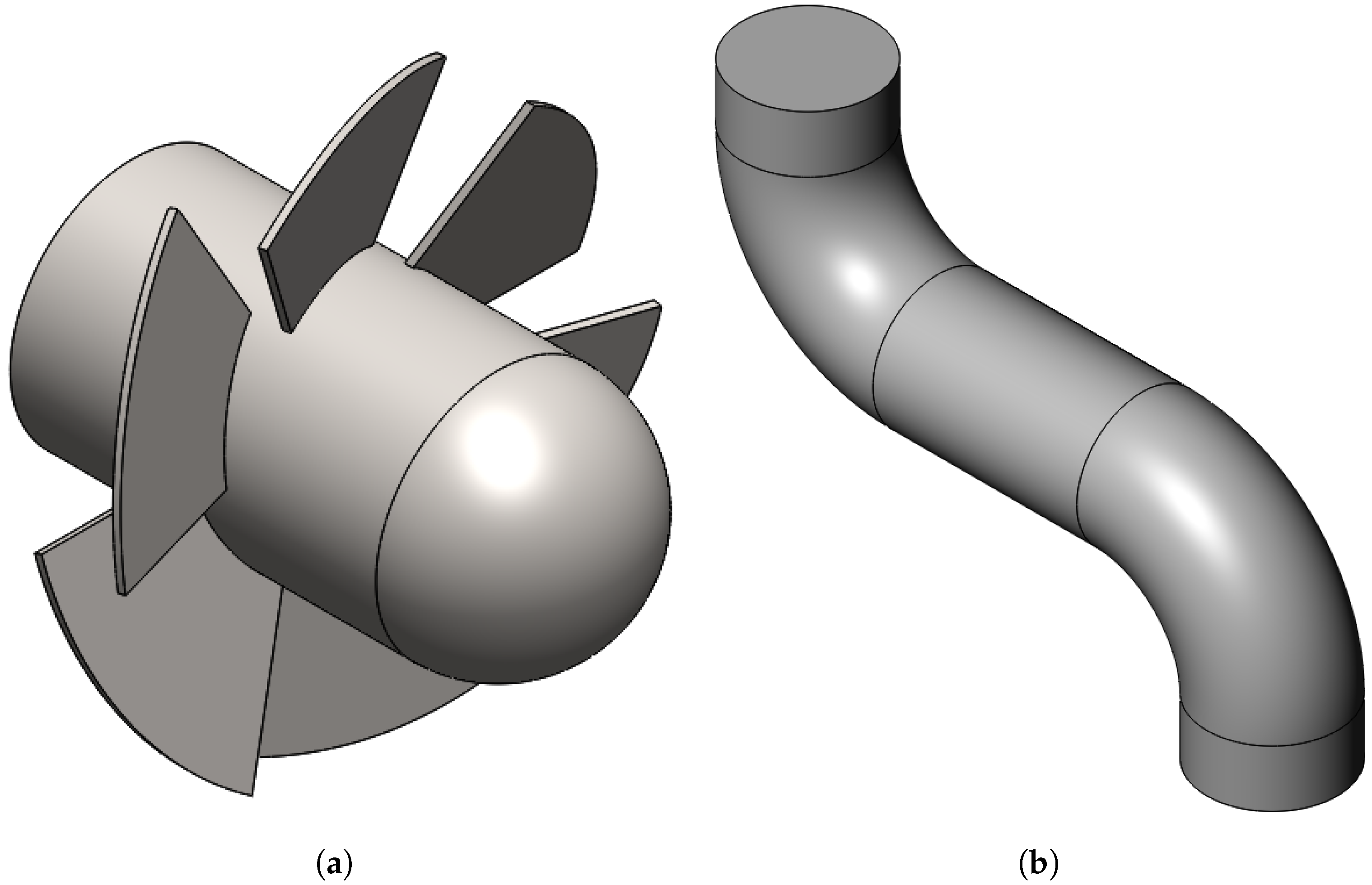
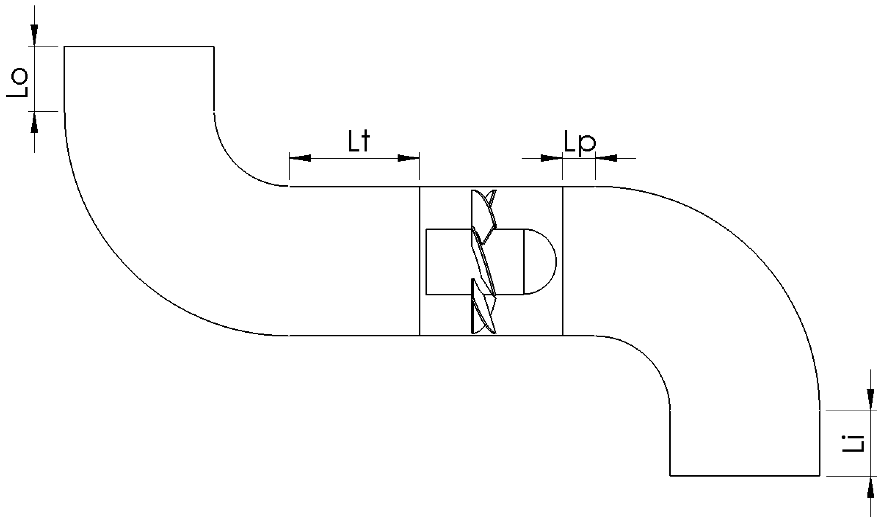
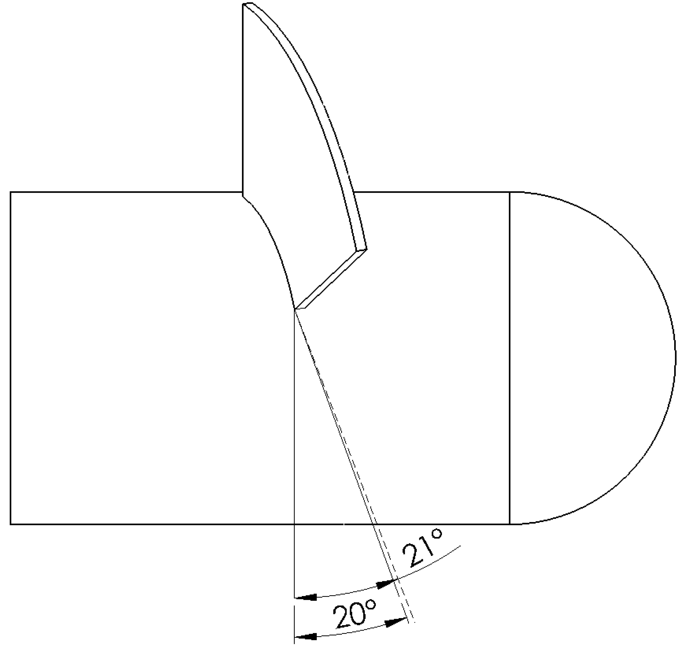
2.1. Research Object

The numerical study was carried out on an axial fan (see Figure 1) with a diameter of 220 mm and a rotational speed of 3000 revolutions per minute, installed in a pipe of a circular cross-section with a diameter of 230 mm. The rotor has six blades on a hub with a diameter of 100 mm and a length of 200 mm at an angle of 20${}^{\circ }$. For such an assumed rotational speed, the fan achieves a volume flow rate of 750 m${}^3·$h${}^{-1}$.

The numerical model was a computational grid consisting of 2,120,050 cells, in which the Navier–Stokes equations were solved using the finite volume method. The main fan parameters are shown in

Table 1. Parameters of the axial fan.

Parameter	Symbol	Unit	Value
Rotational speed	n	r·min${}^{-1}$	3000
Number of blade	z	-	6
Rotor diameter	D	mm	220
Hub diameter	$D_h$	mm	100
Hub length	$H_l$	mm	200
Inlet/outlet diameter	$D_i$/$D_o$	mm	230
Inlet/outlet length	$L_i/L_o$	mm	100
Blade angle	$\theta$	${}^{\circ }$	20

.

In the model, two characteristic zones can be identified: a rotating zone in which the rotor is located and a stationary zone representing a curved pipeline. The geometric model does not include the fan fixing elements inside the pipeline. To simplify the model, steering systems and airflow straightening elements were also omitted. Marked in Figure 2, distances $L_p$ and $L_t$ are equal to each other and are 70.16 mm. Inlet straight sections $L_i$ and outlet $L_o$ of the pipeline are equal and amount to 100 mm.

The geometric model of the rotor was made in SolidWorks and then adapted to the ICEM CFD environment. The ICEM CFD program was used to create a orthogonal computational mesh based on a multi-block structure grids topology. In the areas close to the leading and trailing edges, vortices were created due to the separation of the boundary layer, which is why the computational grid was appropriately compacted at these points in order to solve the flow with greater precision. In addition, a wall layer was modeled to provide a parameter $y^{+}<5$. In order to analyze the validity of the model performed, an analysis of the independence of the results from the calculation grid was performed. The mesh used (see Figure 3) allowed for results of sufficient accuracy to be obtained in a reasonable time.

2.2. Mathematical Model

The first and very important step in the simulation is to locate the sources that can be used to calculate the generated noise. This can be achieved using appropriate computational fluid dynamics techniques. In this field, the basic equations are based on the Navier–Stokes equations derived from the conservation of mass (continuity equation), conservation of momentum, and conservation of energy.

The continuity equation can be written for fluids as:

$$\rho \frac{\partial u_i}{\partial x_i}=0$$

(1)

where $\rho$ is the density of the fluid, t is the time, components of the velocity vector $\mathbf{u}$ in the coordinate system, and $x_i$ coordinates in the Cartesian system. The momentum equation is written as:

$$\rho \frac{\partial u_i}{\partial t}+\rho \frac{\partial u_i{u}_j}{\partial x_j}=-\frac{\partial p}{\partial x_i}+\frac{\partial {\tau }_{ij}}{\partial x_j},$$

(2)

where p is the pressure and ${\tau }_{ij}$ are viscous stresses. Equation (2) is derived by applying Newton’s second law of dynamics, which relates the forces acting on a fluid volume to its acceleration.

Turbulence model $k-\omega$ is one of the most popular models, which shows the phenomena of turbulent flow. It belongs to a family of models in which all turbulence effects are modeled. This is a two equation model. This means that the transport equations are solved to include phenomena, such as convection and turbulent energy dissipation. The variables considered in the equation are the turbulent kinetic energy k, representing the turbulence energy, and the specific turbulent dispersion coefficient $omega$, denoting the dispersion rate of the turbulence kinetic energy. Variable $\omega$ is also known as the turbulence scale. The standard $k-omega$ model works well for low Reynolds number flows where the boundary layer is appropriately sized and the viscous sublayer is well separated. Thus, the standard model $k-\omega$ is best suited for modelling the boundary layer. Other advantages include excellent performance in complex near-wall flows with adverse pressure gradients and separation, e.g., in rotating machinery. The model also predicts excessive and early vortex separations.

Model $k-\omega$ SST is a model that offers the strengths of the $k-ϵ$ proposed by Launder and Spalding [32] and model $k-\omega$ proposed by Wilcox [33], and provides an additional component to limit the overproduction of turbulent kinetic energy in areas of high pressure gradients (stagnation points, areas of separation vortex near wall layer). Menter [34] examining models $k-ϵ$ and $k-\omega$, and observed that the first handles turbulence well in free and shear layers and shows negligible sensitivity to inlet boundary conditions for quantities describing turbulent flow. This is a desirable quality because these quantities are often not exactly known in practical calculations. However, the $k-\omega$ model better models turbulent flow in the boundary layer but is more sensitive in free flow.

The sound pressure level (SPL) was determined using the FW-H analogy. This model is based on the Lighthill analogy and allows noise to be determined by equivalent acoustic sources. Ansys Fluent uses these equations to determine the sound pressure at a given distance from a sound source by an integral over the surface containing those sources. The FW-H equation is a non-homogeneous wave equation [7,35], which can be derived by combining the continuity and Navier–Stokes equations. It can be written as

$$\begin{array}{cc}\hfill \frac{1}{a_0^2}\frac{{\partial }^2{p}^{\prime }}{\partial t^2}-{\nabla }^2{p}^{\prime }& =\frac{{\partial }^2}{\partial x_i\partial x_j}\left\{T_{ij}H\left(f\right)\right\}\hfill \\ \hfill & -\frac{\partial }{\partial x_i}\left\{\left|P_{ij}{n}_j+\rho u_i\left(u_n-v_n\right)\right|\delta \left(f\right)\right\}\hfill \\ \hfill & +\frac{\partial }{\partial t}\left\{\left|{\rho }_0{v}_n+\rho \left(u_n-v_n\right)\right|\delta \left(f\right)\right\}\hfill \end{array}$$

(3)

where $u_i$—air velocity in the direction of $x_i$, $v_i$—surface velocity in the direction of $x_i$, $u_n$—air velocity normal to the surface $f=0$, $\delta \left(f\right)$—Dirac delta, $v_n$—velocity of the surface normal to the surface, $H\left(f\right)$—Heaviside function, $p^{\prime }$—sound pressure in the far field $(p^{\prime }-p_0)$, $n_i$—normal vector pointing to the external area $(f>0)$, $a_0$—speed of sound in the far field, $Pij$—compressive stress tensor, $T_{ij}$—Lighthill stress tensor.

To solve Equation (3), the Green’s function must be used to the open area. The complete solution involves the calculation of surface and volume integrals, the first representing monopole, dipole, and partially quadrupole acoustic sources, and the second representing quadrupole sources in the area outside of the source surface. The volume integral becomes negligible when the Mach number value of the flow is small and the source area covers the source area. In Ansys Fluent, choosing a source on a solid surface-like rotor, the volume integrals are neglected, then the equation takes the following form:

$$p^{\prime }=(\overrightarrow{x},t)=p_T^{\prime }(\overrightarrow{x},t)p_L^{\prime }(\overrightarrow{x},t)$$

(4)

$$\begin{array}{cc}\hfill 4\pi p_T^{\prime }(\overrightarrow{x},t)& ={\int }_{f=0}\left[\frac{{\rho }_0\left({\dot{U}}_n+U_{\dot{n}}\right)}{r{\left(1-M_r\right)}^2}\right]dS\hfill \\ \hfill & +{\int }_{f=0}\left[\frac{{\rho }_0{U}_n\left\{r{\dot{M}}_r+a_0\left(M_r-M^2\right)\right\}}{r^2{\left(1-M_r\right)}^3}\right]dS\hfill \end{array}$$

(5)

$$\begin{array}{cc}\hfill 4\pi p_L^{\prime }(\overrightarrow{x},t)& =\frac{1}{a_0}{\int }_{f=0}\left[\frac{{\dot{L}}_r}{r{\left(1-M_r\right)}^2}\right]dS\hfill \\ \hfill & +{\int }_{f=0}\left[\frac{L_r-L_M}{r^2{\left(1-M_r\right)}^2}\right]dS\hfill \\ \hfill & +\frac{1}{a_0}{\int }_{f=0}\left[\frac{L_r\left\{r{\dot{M}}_r+a_0\left(M_r-M^2\right)\right\}}{r^2{\left(1-M_r\right)}^3}\right]dS\hfill \end{array}$$

(6)

where

$$U_i=v_i+\frac{\rho }{{\rho }_0}\left(u_i-v_i\right)$$

(7)

$$L_i=P_{ij}{\widehat{n}}_j+\rho u_i\left(u_n-v_n\right)$$

(8)

The contribution of quadrupole terms (volume integrals) in the FW-H analogy is proportional to the square of the Mach number ($M^2$). In the analyzed system, the Mach number reaches values below 0.1, which means that the volume integrals can be omitted. Considering the time t and a distance to the observer r, the integral equation takes into account the delay due to the distance from the source to the receiver, according to the following formula:

$$\tau =t-\frac{r}{a_0}$$

(9)

$$\begin{array}{c}{M}_r=M_i{r}_i{\dot{M}}_r=\frac{\partial M_i}{\partial \tau }{r}_i\hfill \\ Q_n=Q_i{\widehat{n}}_i{\dot{Q}}_n=\frac{\partial Q_i}{\partial \tau }{\widehat{n}}_i{Q}_{\dot{n}}=Q_i\frac{\partial {\widehat{n}}_i}{\partial \tau }\hfill \\ L_i=L_{i}j{\widehat{n}}_i{\dot{L}}_r=\frac{\partial L_i}{\partial r}{\dot{r}}_i{L}_r=L_i{\widehat{r}}_i{L}_M=L_i{M}_i\hfill \end{array}$$

(10)

where $\overrightarrow{n},\overrightarrow{r}$—unit vectors of radiation and normal to the wall, M—Mach number of the surface source velocity component along the direction of the radiation vector.

2.3. Boundary Conditions and Solver Settings

The calculations started by simulating free flow, i.e., forced only by a rotating impeller at 3000 r·min${}^{-1}$ around the X axis. For this purpose, boundary conditions of 0 Pa corresponding to atmospheric pressure were applied at the inlet and outlet, respectively. To reduce calculation time, the strategy involves running the simulation at a steady state (MRF) for about 500 iterations until the solution converges below ${10}^{-4}$ and then take the results as initial conditions for the unsteady simulation (sliding mesh) with a time step of $5.5·{10}^{-5}$ s, which corresponds to 360 time steps per rotation of the rotor. Since the Mach number value was approximately 0.1, the flow was assumed to be incompressible, reducing the computational resources required and the computation time. The calculation used the FW-H equation implemented in Ansys Fluent based on Lighthill’s acoustic analogy. The rotor and the pipeline walls are indicated as sources of sound (control surface). As receivers, 510 points were selected and placed on a sphere with a radius of 3 m where the acoustic pressure was computed (Figure 4).

The resulting sound pressure obtained in the time domain was subjected to Fourier analysis. The boundary conditions are shown in

Table 2. Boundary Conditions.

Boundary Condition	Symbol	Unit	Value/Zone
Operating pressure	$P_{atm}$	Pa	101,325
Inlet pressure	$P_i$	Pa	0
Outlet pressure	$P_o$	Pa	0
Mesh motion	n	r·min${}^{-1}$	3000
Interface	-	-	rotor/duct contact area
Wall	-	-	rotor/duct walls
Time step	t	s	$5.5·{10}^{-5}$

.

To obtain the fan characteristics, calculations were performed for 20 various volume flow rate values in the range of $0.0997÷0.1994$ m${}^3·$s${}^{-1}$, of which the points marked $1÷4$ turned out to be a stall range, while the range $5÷20$ determined the operating range of the fan. In order to improve the readability of the presented graphs, we decided not to include characteristic points from the stall range on the graphs.

Table 3. Measurement points.

Nr	Volume Flow Rate (m${}^3$/s)	Percentage (%)	Nr	Volume Flow Rate (m${}^3$/s)	Percentage (%)
1	0.0997	50.00	11	0.1770	88.75
2	0.1097	55.00	12	0.1795	90.00
3	0.1196	60.00	13	0.1820	91.25
4	0.1246	62.50	14	0.1845	92.50
5	0.1595	80.00	15	0.1869	93.75
6	0.1645	82.50	16	0.1894	95.00
7	0.1670	83.75	17	0.1919	96.25
8	0.1695	85.00	18	0.1944	97.50
9	0.1720	86.25	19	0.1969	98.75
10	0.1744	87.50	20	0.1994	100.00

shows the calculation points and the corresponding percentage of unthrottled flow.

A pressure-based coupled algorithm was used to perform the calculations. The pressure-based solver uses an algorithm called the projection method, which solves the continuity and momentum equations [36]. The equation of momentum is calculated by the second-order upwind scheme [37].

3. Results

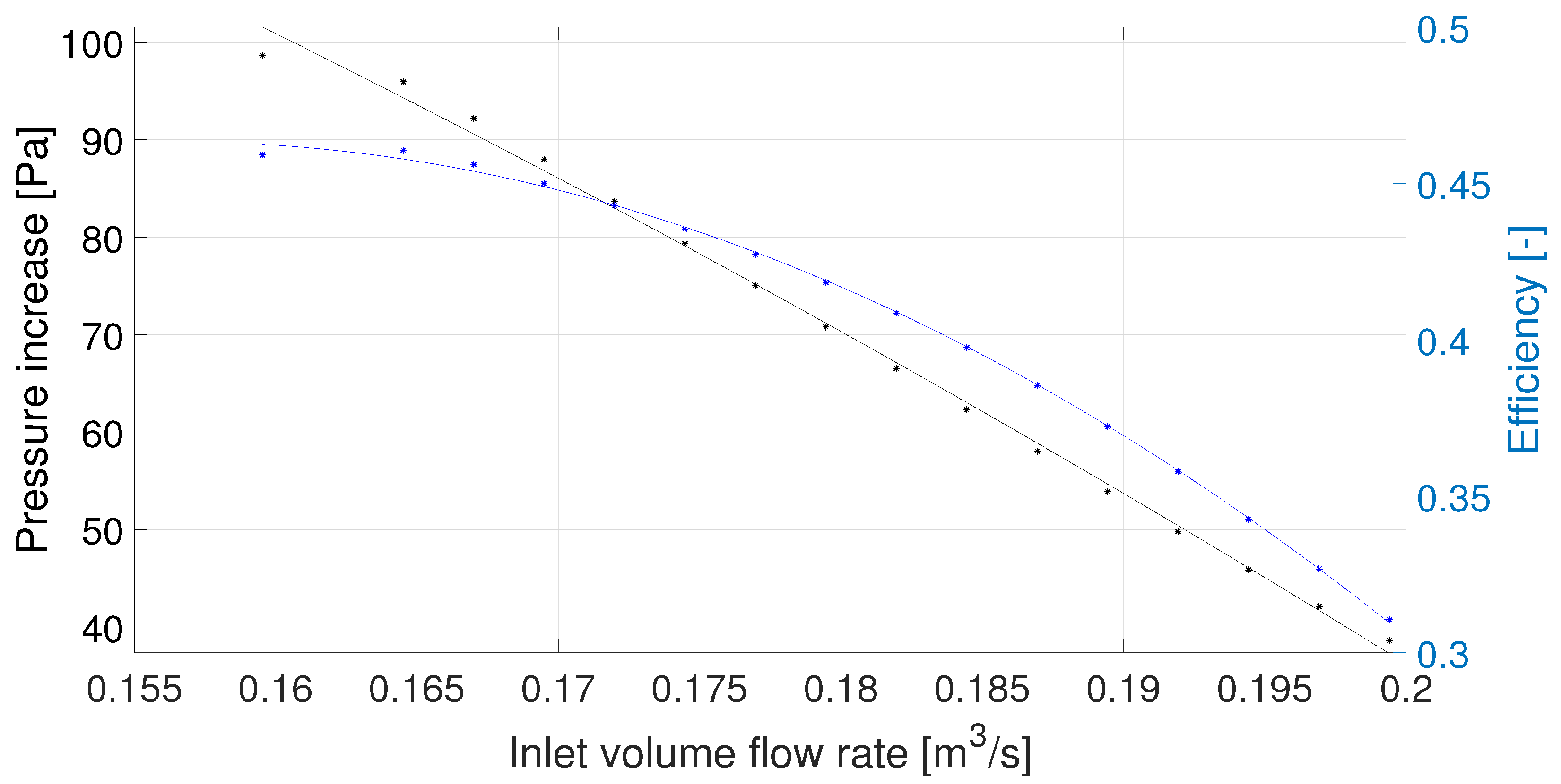
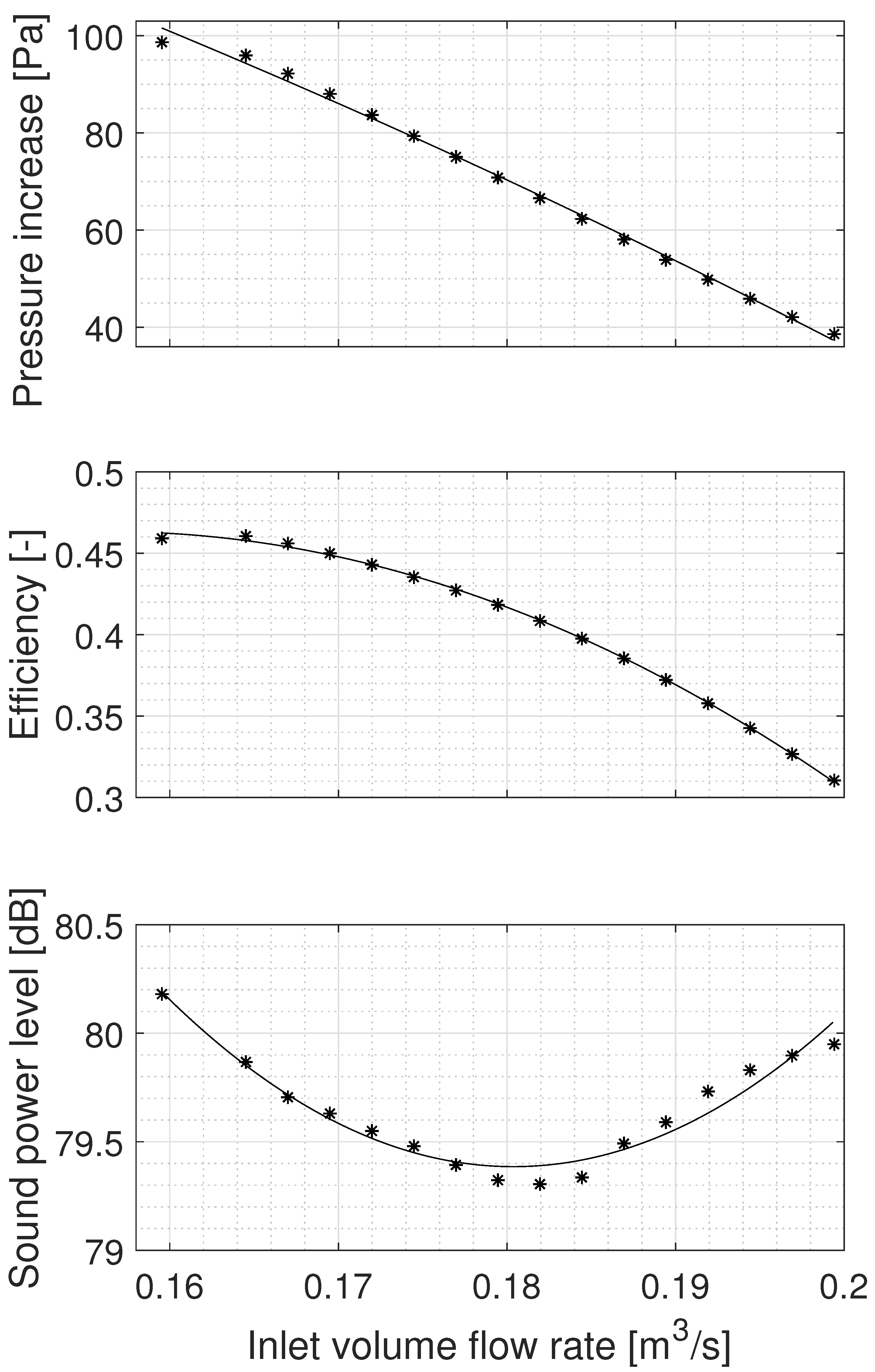
3.1. Fan Characteristics

The numerical calculations were completed after 7200 time steps, which corresponds to 20 rotations of the rotor. The flow is established after approximately 1000 steps. The total pressure increase $\Delta p$ was used as a criterion for flow stabilization. The velocity contours of the resolved flow are shown in Figure 5.

On the basis of the obtained results, the basic parameters of the fan were calculated to determine its characteristics. The formula was used to calculate the mechanical power

$$N_m=M\omega$$

(11)

where M is the torque on the rotor expressed in [Nm] and $\omega$ is the angular velocity expressed in [rad·s${}^{-1}$]. The effective power was calculated as

$$N_u=\Delta p\dot{V}$$

(12)

where $\Delta p$ is the pressure increase and $\dot{V}$ is the volume flow rate behind the rotor. Due to the low compression, the compressibility of the medium is not taken into account. The efficiency was calculated according to the equation

$$\eta =\frac{N_u}{N_m}$$

(13)

In Figure 6, it can be seen that points $1÷4$ present a pressure increase significantly different from the rest of the measurement points and reach $\Delta p=185.2÷215.7$ Pa and their amplitude is approximately approximately 20 Pa, while the amplitude at the points $5÷20$ is only 2 Pa. The results of the calculations of pressure increase and efficiency are shown in Figure 7.

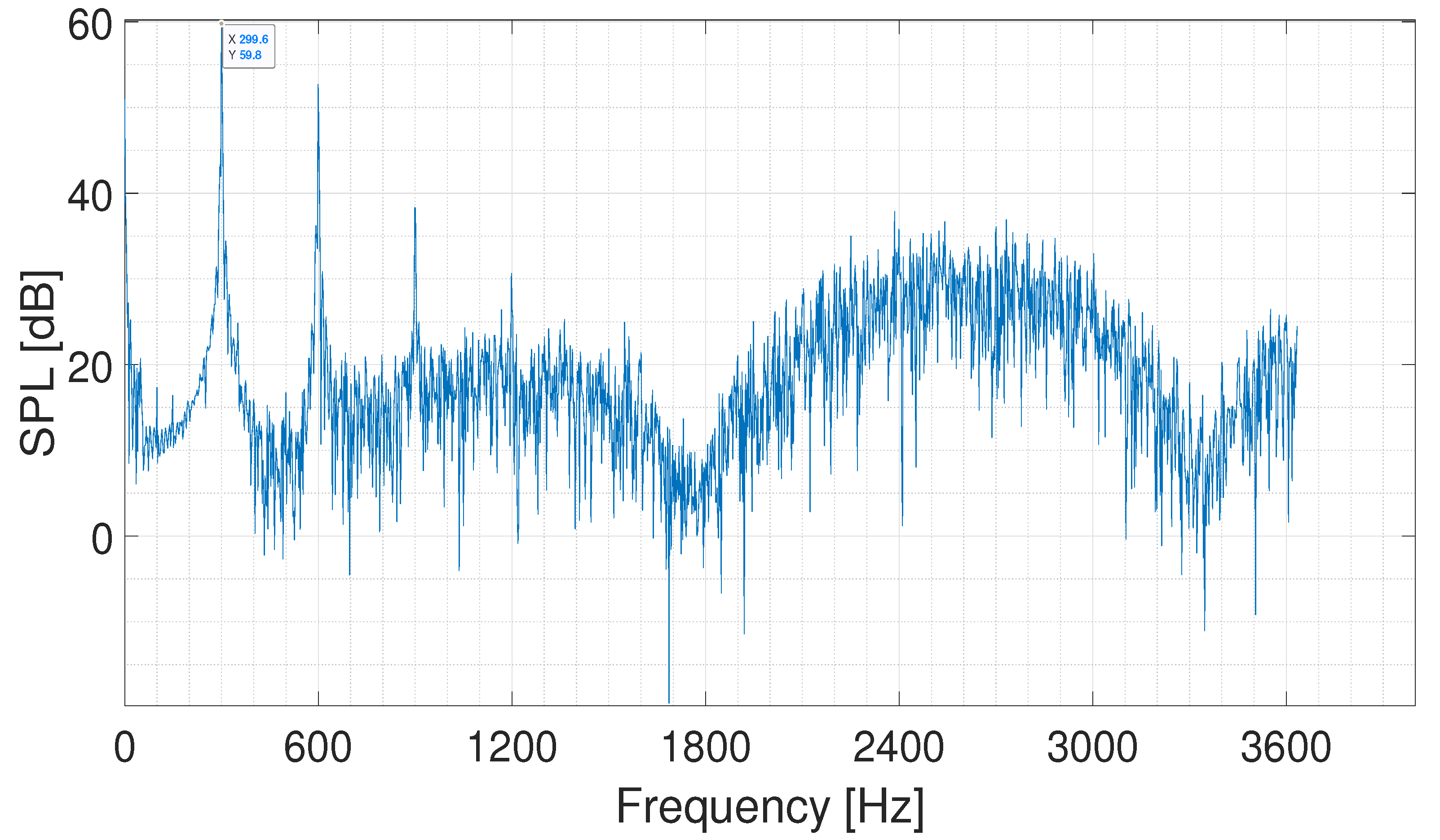
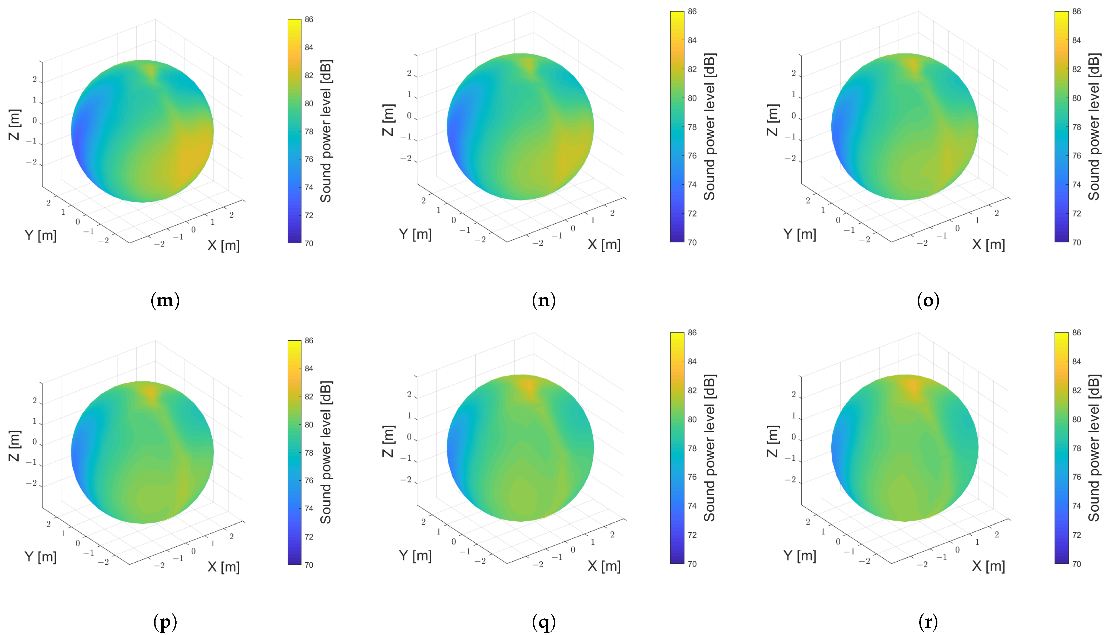
3.2. Aerodynamic Noise Characteristics

The acoustic power of the fan during its operational conditions was determined. Therefore, distributions of the fluid pressure and velocity around the fan in the duct in successive moments was calculated. Next, the FW-H analogy was used to determine the sound pressure values in points on the sphere around the fan. In this case, reflections from walls of the duct were not taken into account because the radiated power is a parameter of the acoustic source. At low sound pressures and the assumption of unidirectional coupling between the flow and the acoustic field, the reflections do not have much of an impact on the power of the source itself. The considerable size of the sphere was necessary to be able to treat the acoustic wave as locally plane in the receivers. Using the FW-H analogy, a time domain acoustic signal was obtained on the surface of a sphere of radius R = 3 m. On this area, 510 receivers were placed in which the acoustic signal was obtained. Sound pressures were determined at the measurement points, from which the sound intensity was calculated assuming that the wave was locally flat. The integral of the intensity along the surface of the sphere gives the sound power value. The acoustic pressure was determined in each of the receivers, and assuming a locally plane wave, on this basis the sound intensity was calculated. The receivers on the sphere were evenly distributed and each was assigned to a sphere surface element. Integration was performed using the rectangle rule (the value of the intensity in the receiver multiplied by the surface element assigned to a given node) [38]

$$SWL=10{\log }_{10}\left(\frac{P}{P_0}\right)$$

(14)

where $P_0$ is the reference power equal to ${10}^{-12}W$ and P is the power of sound expressed by the formula

$$P={\oint }_{A}IdA={\oint }_A\frac{p^2}{{\rho }_{0}c}dA\approx \frac{{\sum }_i{A}_i{p}_i^2}{{\rho }_{0}c}$$

(15)

where A is the surface area, $p_{rms}$ is the root mean square of the sound pressure, $\rho$ = 1.1225 kg/m${}^3$ is the density of air, $c=340$ m/s is the speed of sound. On the basis of the calculated values of the sound pressure, calculations were carried out to obtain the sound pressure level.

$$SPL=20{\log }_{10}\left(\frac{p_{rms}}{p_{ref}}\right)$$

(16)

In addition, a Fourier analysis was carried out to verify the blade pass frequency calculated from the relationship

$$BPF=\frac{RPM\times z}{60}$$

(17)

where $p_{ref}$ is the reference pressure equal to $2·{10}^{-5}$ Pa. The results are shown in Figure 8, showing the blade pass frequency of 300 Hz and its harmonics.

The results obtained are compared with the fan characteristics in Figure 9. From the results obtained, it can be concluded there is a significant increase in the sound power level in the stall area compared to the working area, which is up to 10 dB. In the operating area, the sound power level is in the range 79.3 ÷ 90.9 dB (see

Table 4. SWL results.

Nr	SWL [dB]	Nr	SWL [dB]
1	88.47	11	79.39
2	89.96	12	79.32
3	90.88	13	79.30
4	90.80	14	79.33
5	80.18	15	79.49
6	79.87	16	79.59
7	79.70	17	79.73
8	79.63	18	79.83
9	79.55	19	79.90
10	79.48	20	79.95

) and can be approximated by a parabola with a local minimum. In experimental work [39], a similar character of sound power level was obtained.

From the resulting sound pressure level distribution shown in Figure 10, it can be seen that there are negligible differences in cases 5–20. A common feature of all cases is a higher sound pressure level on the upstream side and around the X axis at the height of the blades. In cases 1–4, the sound pressure level is much higher than in the other cases, and it is related to greater pressure fluctuation in the stall area.

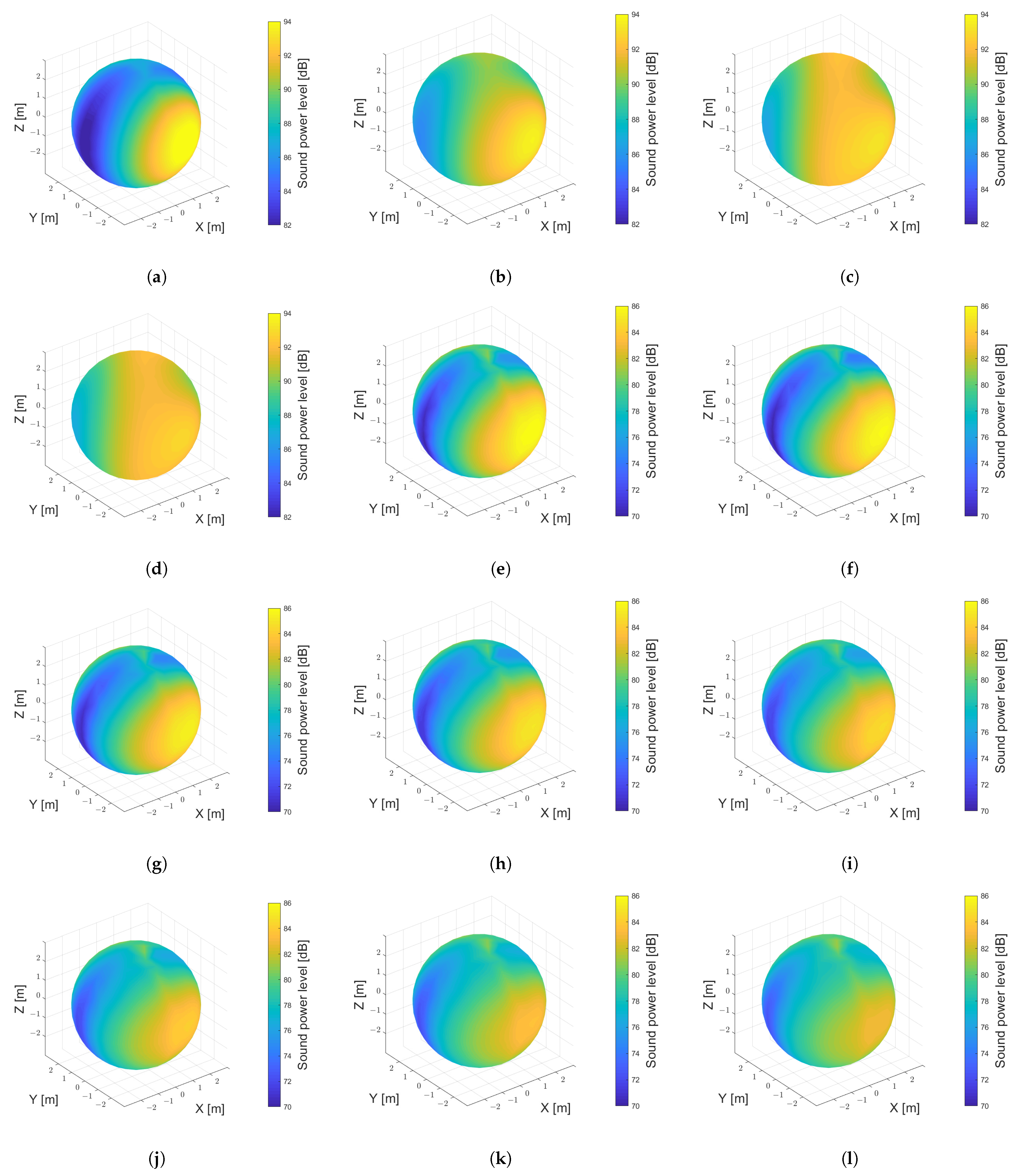
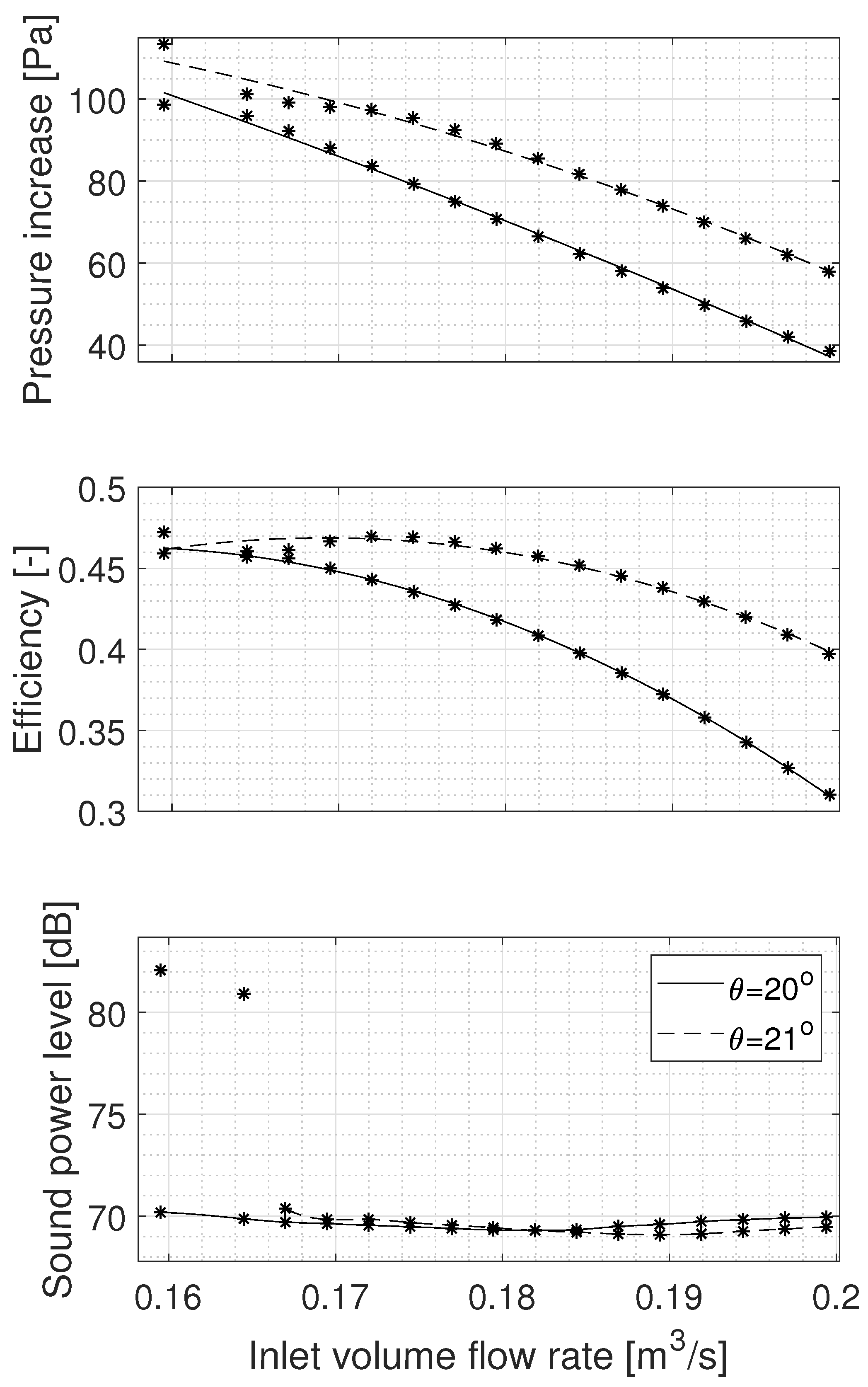
3.3. Sensitivity of the Fan Parameters to the Change of the Blade Angle

The study investigated the sensitivity of the fan characteristics to a change in the blade angle. For this purpose, we carried out additional numerical calculations for the blade angle $\theta ={21}^{\circ }$ (Figure 11).

The sensitivity of a characteristic function to changes in a design parameter can be defined as the partial derivative of the function describing that characteristic, with respect to that parameter. The sensitivity coefficients, in normalized form, can be found as

$$S_x^y=\frac{\partial y_i/y_i}{\partial x_j/x_j}$$

(18)

where $S_x^y$ is the normalized sensitivity coefficient, $y_i$ is model dependent variable and $x_j$ is input parameter.

$$S_{\theta }^{\Delta p}=\frac{\partial p/p}{\partial \theta /\theta }\approx \frac{\Delta p/p}{\Delta \theta /\theta }=0.2416$$

(19)

$$S_{\theta }^{\eta }=\frac{\partial \eta /\eta }{\partial \theta /\theta }\approx \frac{\Delta \eta /\eta }{\Delta \theta /\theta }=0.1042$$

(20)

$$S_{\theta }^{SWL}=\frac{\partial SWL/SWL}{\partial \theta /\theta }\approx \frac{\Delta SWL/SWL}{\Delta \theta /\theta }=-5.9558·{10}^{-5}$$

(21)

The values from points $8÷16$, which constitute the work area, were used for the calculations. Two single $(\ast )$ symbols define the beginning of a new stall zone (see Figure 12).

4. Conclusions

Computer simulations using CFD techniques were carried out to investigate the noise generated by the axial fan. The URANS time-averaging method and the FW-H analogy implemented in Ansys Fluent were used in the calculations. Using these methods, the sound pressure was calculated on a sphere with a radius of 3 m from the sound source, from which the acoustic characteristics were determined and an FFT analysis was performed. The analysis was carried out for twenty characteristic points for two different blade angles. The main conclusions of the numerical analysis are presented below.

On the basis of the torque and total pressure increase analysis, the stall area can be verified for the operating points $1÷4$ and normal work in points $5÷20$. In the stall region, the total pressure increase is $\Delta p=185.2÷215.7$ Pa, while in the normal operating area, it is $79.8÷99.8$ Pa.

Fourier analysis, calculated using the FW-H acoustic analogy of the acoustic pressure, made it possible to determine the blade pass frequency equal to 300 Hz and its harmonics, which allows to confirm the accuracy of the numerical simulations.

As expected, the determined characteristics show that the fan efficiency increases with increasing total pressure increase.

The difference in the indicated sound power level in the test area is just 1 dB. However, attention should be paid to the obtained characteristics of the sound power level, which in the studied area has a local minimum, which encourages additional considerations on determining the optimal operating point for which the emitted noise is the lowest.

The determined sound power level on a sphere with a radius of 3 m from the noise source indicates higher emission from the upstream, which may be caused by turbulent flow caused by the curved pipeline. The common feature of the presented results is a greater level of generated noise around the X axis at the height of the blades.

From the simulations carried out for a variable blade angle, it can be seen that, for angle $\theta ={21}^{\circ }$ at certain points of the characteristic curve, the fan efficiency increases from $2\%$ to $8\%$. A sound power level at an angle of $\theta ={21}^{\circ }$ emits 1 dB less at certain points than for angle $\theta ={20}^{\circ }$.

For blade angle $\theta ={21}^{\circ }$, the characteristic point that defines the stall zone has moved, and for this, the angle is located between the points $1÷6$.

The generated noise is influenced by many more design and operational parameters of the axial fan. The aim of the article was to show the change in the angle of the rotor blades in the entire exploitation area, i.e., with a variable flow rate. The calculations consist of examining more than 20 measurement points for one parameter change, which require a lot of computational time, but they are planned for the second part of the research. Further experiments on the real object will be aimed at verifying the numerical model and extending the research with parameters influencing the generated noise.

References

1. Czajka, I. Modeling of Acoustic Phenomena in Aerodynamic Flows; Volume 365, Dissertations, Monographs; AGH: Krakow, Poland, 2019. [Google Scholar]
2. Kissner, C.; Guérin, S.; Seeler, P.; Billson, M.; Chaitanya, P.; Carrasco Laraña, P.; de Laborderie, H.; François, B.; Lefarth, K.; Lewis, D.; et al. ACAT1 Benchmark of RANS-Informed Analytical Methods for Fan Broadband Noise Prediction—Part I—Influence of the RANS Simulation. Acoustics 2020, 2, 539–578. [Google Scholar] [CrossRef]
3. Lighthill, M.J. On sound generated aerodynamically I. General theory. Proc. R. Soc. Lond. Ser. A Math. Phys. Sci. 1952, 211, 564–587. [Google Scholar] [CrossRef]
4. Lighthill, M.J. On sound generated aerodynamically II. Turbulence as a source of sound. Proc. R. Soc. Lond. Ser. A Math. Phys. Sci. 1954, 222, 1–32. [Google Scholar] [CrossRef]
5. Lighthil, M.J. Jet Noise. AIAA J. 1963, 1, 1507–1517. [Google Scholar] [CrossRef]
6. Curle, N. The influence of solid boundaries upon aerodynamic sound. Proc. R. Soc. Lond. Ser. A Math. Phys. Sci. 1955, 231, 505–514. [Google Scholar] [CrossRef]
7. Williams, J.F.; Hawkings, D.L. Sound generation by turbulence and surfaces in arbitrary motion. Philos. Trans. R. Soc. Lond. Ser. A Math. Phys. Sci. 1969, 321–342. [Google Scholar] [CrossRef]
8. Williams, J.F.; Hawkings, D. Theory relating to the noise of rotating machinery. J. Sound Vib. 1969, 10, 10–21. [Google Scholar] [CrossRef]
9. Schmitz, F.; Yu, Y. Transonic Rotor Noise: Theoretical and Experimental Comparisons; National Aeroacoustics and Space Administration: Washington, DC, USA, 1982; pp. 319–330. [Google Scholar]
10. Brentner, K.S.; Farassat, F. Modeling aerodynamically generated sound of helicopter rotors. Prog. Aerosp. Sci. 2003, 39, 83–120. [Google Scholar] [CrossRef] [Green Version]
11. Konstantinov, M.; Wagner, C. Numerical Simulation of the Sound Generation and the Sound Propagation from Air Intakes in an Aircraft Cabin; New results in numerical and experimental fluid mechanics XI; Springer: Cham, Switzerland, 2018. [Google Scholar] [CrossRef] [Green Version]
12. Sundström, E.; Semlitsch, B.; Mihăescu, M. Acoustic signature of flow instabilities in radial compressors. J. Sound Vib. 2018, 434, 221–236. [Google Scholar] [CrossRef]
13. Al-Am, J.; Clair, V.; Giauque, A.; Boudet, J.; Gea-Aguilera, F. A Parametric Study on the LES Numerical Setup to Investigate Fan/OGV Broadband Noise. Int. J. Turbomach. Propuls. Power 2021, 6, 12. [Google Scholar] [CrossRef]
14. Guérin, S.; Kissner, C.; Seeler, P.; Blázquez, R.; Carrasco Laraña, P.; de Laborderie, H.; Lewis, D.; Chaitanya, P.; Polacsek, C.; Thisse, J. ACAT1 Benchmark of RANS-Informed Analytical Methods for Fan Broadband Noise Prediction: Part II—Influence of the Acoustic Models. Acoustics 2020, 2, 617–649. [Google Scholar] [CrossRef]
15. Biedermann, T.M.; Czeckay, P.; Hintzen, N.; Kameier, F.; Paschereit, C.O. Applicability of Aeroacoustic Scaling Laws of Leading Edge Serrations for Rotating Applications. Acoustics 2020, 2, 579–594. [Google Scholar] [CrossRef]
16. Zhang, X.; Zhang, Y.; Lu, C. Flow and Noise Characteristics of Centrifugal Fan in Low Pressure Environment. Processes 2020, 8, 985. [Google Scholar] [CrossRef]
17. Kholodov, P.; Moreau, S. Identification of Noise Sources in a Realistic Turbofan Rotor Using Large Eddy Simulation. Acoustics 2020, 2, 691–706. [Google Scholar] [CrossRef]
18. Zarri, A.; Christophe, J.; Moreau, S.; Schram, C. Influence of Swept Blades on Low-Order Acoustic Prediction for Axial Fans. Acoustics 2020, 2, 812–832. [Google Scholar] [CrossRef]
19. Zarri, A.; Christophe, J.; Schram, C.F. Low-Order Aeroacoustic Prediction of Low-Speed Axial Fan Noise. In Proceedings of the 25th AIAA/CEAS Aeroacoustics Conference, Delft, The Netherlands, 20–23 May 2019; p. 2760. [Google Scholar] [CrossRef]
20. Herold, G.; Zenger, F.; Sarradj, E. Influence of blade skew on axial fan component noise. Int. J. Aeroacoustics 2017, 16, 418–430. [Google Scholar] [CrossRef]
21. Sanjosé, M.; Moreau, S. Fast and accurate analytical modeling of broadband noise for a low-speed fan. J. Acoust. Soc. Am. 2018, 143, 3103–3113. [Google Scholar] [CrossRef] [PubMed]
22. Ding, H.; Chang, T.; Lin, F. The Influence of the Blade Outlet Angle on the Flow Field and Pressure Pulsation in a Centrifugal Fan. Processes 2020, 8, 1422. [Google Scholar] [CrossRef]
23. Mo, J.o.; Choi, J.h. Numerical Investigation of Unsteady Flow and Aerodynamic Noise Characteristics of an Automotive Axial Cooling Fan. Appl. Sci. 2020, 10, 5432. [Google Scholar] [CrossRef]
24. Zhang, L.; Yan, C.; He, R.; Li, K.; Zhang, Q. Numerical Study on the Acoustic Characteristics of an Axial Fan under Rotating Stall Condition. Energies 2017, 10, 1945. [Google Scholar] [CrossRef] [Green Version]
25. Chan, K.; Saltelli, A.; Scott, E.M. Sensitivity Analysis; Wiley: Chichester, UK, 2000. [Google Scholar]
26. Klieber, M.; Antunez, H.; Hien, T.; Kowalczyk, P. Parameter Sensitivity in Nonlinear Mechanics; Wiley: Chichester, UK, 1997. [Google Scholar]
27. MRÓZ, Z.; HAFTKA, R.T. Sensitivity of buckling loads and vibration frequencies of plates. Stud. Appl. Mech. 1988, 19, 255–266. [Google Scholar]
28. Zheng, C.; Zhao, W.; Gao, H.; Du, L.; Zhang, Y.; Bi, C. Sensitivity analysis of acoustic eigenfrequencies by using a boundary element method. J. Acoust. Soc. Am. 2021, 149, 2027–2039. [Google Scholar] [CrossRef] [PubMed]
29. Romik, D.; Czajka, I.; Suder-Dębska, K. Numerical Investigations of the Design Parameters’ Influence on the Noise of Radial Fan; Polish Acoustical Society, Department of Krakow: Krakow, Poland, 2019; pp. 133–149. [Google Scholar]
30. Romik, D.; Czajka, I. On the Modelling of the Aeroacoustics Phenomena Generated by Axial Fan; AGH: Krakow, Poland, 2019; pp. 122–131. [Google Scholar]
31. Romik, D.; Czajka, I. Influence of Turbulence Models on Numerical Investigation of Axial Fans Efficiency; Department of Power Systems and Environmental Protection Facilities, Faculty of Mechanical Engineering and Robotics, AGH: Krakow, Poland, 2019; pp. 71–79. [Google Scholar]
32. Launder, B.E.; Spalding, D.B. Lectures in Mathematical Models of Turbulence; Launder, B.E., Spalding, D.B., Eds.; Academic Press: London, UK; New York, NY, USA, 1972; p. 7. 169p. [Google Scholar]
33. Wilcox, D.C. Turbulence Modeling for CFD; DCW Industries La Canada: La Canada, CA, USA, 1998; Volume 2. [Google Scholar]
34. Menter, F.R. Two-equation eddy-viscosity turbulence models for engineering applications. AIAA J. 1994, 32, 1598–1605. [Google Scholar] [CrossRef] [Green Version]
35. Brentner, K.S.; Farassat, F. Analytical comparison of the acoustic analogy and Kirchhoff formulation for moving surfaces. AIAA J. 1998, 36, 1379–1386. [Google Scholar] [CrossRef] [Green Version]
36. Chima, R.; Liou, M. Comparison of the AUSM(+) and H-CUSP Schemes for Turbomachinery Applications. In Proceedings of the Computational Fluid Dynamics Conference, Orlando, FL, USA, 23–26 June 2003. [Google Scholar] [CrossRef] [Green Version]
37. Barth, T.; Jespersen, D. The design and application of upwind schemes on unstructured meshes. In Proceedings of the 27th Aerospace Sciences Meeting, Reno, NV, USA, 9–12 January 1989. [Google Scholar] [CrossRef]
38. McAlpine, A. Aeroacoustics of Low Mach Number Flows: Fundamentals, Analysis and Measurement S. Glegg and W. Devenport Academic Press, Elsevier, The Boulevard, Langford Lane, OX5 1GB, Kidlington, Oxford, UK. xiii; 537pp. 2017. Illustrated. £97. ISBN 978-0-12-809651-2. Aeronaut. J. 2018, 122, 2030–2032. [Google Scholar] [CrossRef] [Green Version]
39. Fortuna, S.; Czajka, I. Experimental Verification of Selected Equations Describing the Sound Power Level in Fans. Turbomachinery 2010, nr 138, 21–32. [Google Scholar]
Figure 1. Geometrical model of the fan: (a) rotor, (b) pipeline.
Energies 15 01357 g001
Figure 2. Diagram of built-in fan.
Energies 15 01357 g002
Figure 3. Fan computational grid: (a) rotor mesh, (b) pipeline mesh.
Energies 15 01357 g003
Figure 4. Receivers distribution.
Energies 15 01357 g004
Figure 5. Velocity contours of resolved flow.
Energies 15 01357 g005
Figure 6. Pressure increase.
Energies 15 01357 g006
Figure 7. Pressure increase and efficiency characteristics.
Energies 15 01357 g007
Figure 8. FFT of acoustic signal.
Energies 15 01357 g008
Figure 9. Pressure increase, efficiency, and sound power level characteristics.
Energies 15 01357 g009
Figure 10. Sound power level distribution: (ar) are the measurement points 1–18.
Energies 15 01357 g010aEnergies 15 01357 g010b
Figure 11. Geometry of the model with marked angles θ = 20 and θ = 21 .
Energies 15 01357 g011
Figure 12. Pressure increase, efficiency, and sound power level characteristics for blade angles 20 and 21 .
Energies 15 01357 g012