Yaw Stability Research of the Distributed Drive Electric Bus by Adaptive Fuzzy Sliding Mode Control

Abstract

The direct yaw moment control can effectively enhance the yaw stability of the vehicle under extreme conditions, which has become one of the essential technologies for the distributed driving electric bus. Due to the features of a large mass and high center of gravity of the bus, lateral instability is more likely to occur under extreme driving conditions. To reduce the uncertainty and interference in the yaw movement process of the bus, this paper targets the instability caused by the coupling problem between the sideslip angle and yaw rate. An adaptive fuzzy sliding mode control is proposed to execute direct yaw moment control. The weight coefficient of the sideslip angle and the yaw rate is adjusted via fuzzy control in real time. The optimal direct yaw moment is finally obtained. A distribution method based on the vertical load proportion is adopted for the allocation of four motors’ torque. Under three typical working conditions, a joint simulation test was carried out. The simulation results demonstrate that the raised method decreases the amplitude of the sideslip angle by 20.90%, 12.75%, and 23.67% and the yaw rate is 8.62%, 6.89%, and 9.28%, respectively. The chattering and sudden changes in the additional yaw moment are also lessened. The control strategy can realize the control target, which effectively strengthens the yaw stability of the bus.

1. Introduction

The distributed driving electric bus play a significant role in urban public transportation. Electric buses have the advantage of being environmentally friendly, and also shows a very good dynamic performance [1]. However, the bus has the features of a large quality and high center of mass, which is prone to a loss of stability under extreme conditions, such as emergency steering. If this instability cannot be effectively controlled, serious traffic accidents will occur. Therefore, automobile safety control technology is particularly important. Traditional safety control technology is no longer able to meet the realistic requirements of a distributed drive electric bus. Hence, as an active control method, the function of direct yaw moment control (DYC) of the yaw stability of a bus under extreme conditions has attracted increasingly more attention [2,3].

A significant number of studies have been conducted on the DYC of electric vehicles at home and abroad [4,5,6,7,8]. Direct yaw moment control will generate additional yaw moment. Through the torque distribution method, the calculated additional torque is applied to the wheels. Liu et al. proposed a model-based motion control algorithm designed to change the plane motion state of the vehicle by generating torque increments on each wheel. To solve the optimal torque increment vector, a real-time constrained quadratic programming problem is adopted. This method converts the constraints related to the wheel torque limit, tire friction limit, and wheel skid requirement into the upper and lower limits of the tire longitudinal force increments [9]. Initially, feedback control was often adapted as a way to calculate the direct yaw moment of the upper controller [10,11]. Nonetheless, a satisfactory result still cannot be achieved under complex conditions. For this reason, a joint control strategy was utilized. A neural network-based feedback control was proposed [12,13]. Although the stability of the electric vehicle has been improved to a certain extent, it still cannot meet the requirements in some extreme cases. Some nonlinear control algorithms are gradually being used in DYC to further solve this problem, for example, sliding mode control (SMC) [14], model predictive control [15,16,17], fuzzy control [18], etc.

The strong point of SMC is that it can conquer the instability of the system, and has strong robustness against disturbances. Especially for nonlinear systems, it shows a good control effect. Accordingly, SMC has gradually been widely used in recent years [19]. However, there is still the problem of idealization in the modeling process. The uncertainty caused by this problem requires that the larger switching gain is avoided. However, this would produce inevitable chattering [20]. Tota et al. proposed integral sliding mode control that can simultaneously consider the sideslip angle and yaw rate. This method perfected the tracking performance of the controller under transient conditions and decreased the occurrence of buffeting [21]. In the handling stability controller, Guo et al. proposed a unified yaw rate reference of a varying weight factor to ensure the handling and lateral stability of the vehicle at the same time. On this basis, a new integral triple-step method was proposed to calculate the appropriate direct yaw moment for the ideal vehicle motion. The results showed overall improvements in the vehicle handling, lateral stability, and energy performance [22]. Mousavinejad et al. proposed a vehicle dynamics integrated control algorithm that is coordinated by active steering control and direct yaw moment control. Through integral and non-singular terminal sliding mode control, this method is robust against uncertainty [23].

Fuzzy control is a nonlinear control method. There is no need to establish an accurate mathematical model for the controlled object, and the design can be carried out only according to the relevant control experience of the designer. It adopts language-based design rules. It has the advantages of simple design and easy understanding. Du et al. proposed a fuzzy-driven control strategy. Through the fusion of vehicle driving data, an early warning level model is established, and the fuzzy control method is used to obtain the appropriate torque command under the vehicle operating conditions. Torque optimization is carried out according to different vehicle following characteristics [24]. Zhang et al. proposed a spatiotemporal fuzzy graph convolutional network model based on dynamic feature encoding to achieve accurate traffic prediction. On this basis, a graph generation method based on fuzzy C-means clustering is designed to improve the expressive ability of the spatial correlation between stations in a transportation network [25]. Pu et al. developed a real-time method to estimate multimodal traffic speeds on road networks covered by Wi-Fi and Bluetooth passive sensors. Based on the received signal strength metrics of the Wi-Fi and Bluetooth signals, an algorithm is developed to correct for biased estimated traffic speeds, and a novel semi-supervised possibilistic fuzzy C-means clustering algorithm is proposed to identify the traffic modes of Wi-Fi and Bluetooth device owners [26]. Qi et al. proposed a control strategy that can not only meet the requirements of road conditions and the driver’s driving intention, but also consider the vehicle’s operating state. Using the fuzzy control algorithm, a fuzzy controller is designed, which takes the motor demand variable rate and battery charging state as the input and the motor demand torque compensation coefficient as the output [27].

Although these studies can reduce the occurrence of chattering and effectively improve the lateral stability of the vehicle, the problem of the constant switching gain coefficient, which causes bad system adaptability, has not yet been fully settled. To address this limitation, Sun et al. posed a new adaptive non-singular fast terminal sliding mode control method. The controller effectively lessened the occurrence of buffeting, and significantly decreased the peak values of the sideslip angle and yaw rate [28]. Asiabar et al. put forward a strategy that generated direct yaw moment by adaptive sliding mode control of unknown parameters. This method improved the handling stability of the vehicle [29]. Fu et al. used variable control gain coefficients to adjust to the changes in the sideslip angle, which enhanced the robustness of the vehicle to changes and uncertainties in the parameters [30]. Zhang et al. proposed a fuzzy algorithm to calculate the sliding mode gain coefficient so that it can adjust to the change in the motion state of the vehicle, and improve the adaptability of the system [31]. Even though these studies considered the instability problem caused by coupling between the sideslip angle and yaw rate, they did not take into account the weight between them under different motion situations. This led to the inability to obtain the optimal weighting coefficient of the sideslip angle and yaw rate.

In view of the above research, this paper combines the advantages of fuzzy control and SMC, and designs an adaptive fuzzy sliding mode control (AFSMC) method. This method resolves the buffeting problem produced by the traditional SMC and settles the instability problem caused by the coupling relation between the sideslip angle and yaw rate. On the premise of improving handling stability of bus, AFSMC changes the weight coefficients of the sideslip angle and yaw rate through a fuzzy algorithm. This can decrease the chattering and harmful sudden changes and reinforce the system adaptability. It offers a basis for actual engineering applications.

This article also has the following parts: Section 2 establishes the two degrees of freedom (2-DOF) and seven degrees of freedom (7-DOF) vehicle model. Section 3 describes how the controller is designed in detail and the torque distribution method. Then, joint simulation tests are implemented, and the simulation results are analyzed and discussed. Section 4 summarizes the research of this article.

2. Bus Dynamic Models

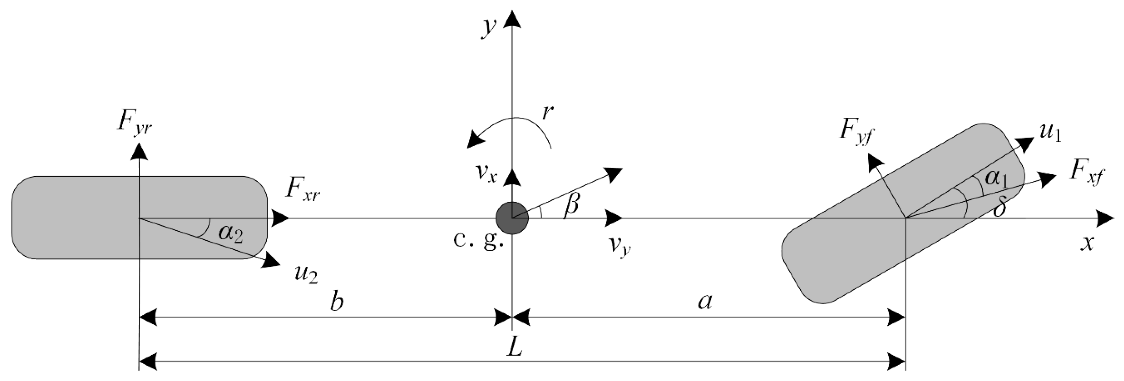
2.1. Two Degrees of Freedom Bus Model

To easily explain the characteristics of yaw motion of the vehicle, we construct a bus model to simplify the linear 2-DOF model. The values of the parameters derived from this model are used as reference values for subsequent controllers. The input to this model is the front wheel angle. These two degrees of freedom are lateral motion along the y-axis and yaw rotation around the z-axis, respectively.

The model has the following assumptions:

(1)

The vehicle only makes plane motion.

(2)

The roll angle, pitch angle, and vertical displacement are all zero.

(3)

The longitudinal speed is constant.

(4)

Only the lateral and yaw motions are considered, so the influence of the shift of the longitudinal axle load is ignored.

Figure 1 shows the force analysis. The dynamic equations of the vehicle motion are:

$$\{\begin{array}{c}\left(k_1+k_2\right)\beta +\frac{a{k}_1-b{k}_2}{v_x}r-k_1\delta =m\left({\dot{v}}_y+v_{x}r\right)\\ \left(a{k}_1-b{k}_2\right)\beta +\frac{a^2{k}_1+b^2{k}_2}{v_x}r-a{k}_1\delta =I_Z\dot{r}\end{array}$$

(1)

where ν_x is the longitudinal speed; ν_y is the lateral speed; r is the yaw rate; δ is the front steering wheel angle; and β is the sideslip angle of the center of mass.

Table 1. The basic parameters of the distributed drive electric bus.

Parameters	Symbols	Values
Bus mass	m	7620 kg
Distance from the center of mass to the front axle	a	3105 mm
Distance from the center of mass to the rear axle	b	1385 mm
Cornering stiffness of the front tire	k1	−140,550 N/rad
Cornering stiffness of the rear tire	k2	−140,550 N/rad
Yaw moment of inertia	IZ	30,782.4 kg·m2
Wheelbase	d	2030 mm
Height of the center of mass	hg	1200 mm
Wheel radius	Re	510 mm

shows the definitions and values of the other basic parameters of the distributed drive electric bus.

The model has a few virtues, for instance, low complexity, simple structure, and good real-time performance. It can commendably describe the relevance between the handling stability and yaw rate and sideslip angle of the vehicle. Therefore, it can be regarded as an ideal state of motion. The values of the parameters obtained from this model are used as the ideal values in the controller as a reference.

In the steady state, the desired sideslip angle and desired yaw rate are:

$$\{\begin{array}{c}{r}_d=\frac{v_x}{L\left(1+K{v}_x^2\right)}\delta \\ {\beta }_d=\frac{b+\frac{ma{v}_x^2}{k_{2}L}}{L\left(1+K{v}_x^2\right)}\delta \end{array}$$

(2)

where r_d is the desired yaw rate and β_d is the desired sideslip angle. K is the insufficient steering coefficient:

$$K=\frac{m}{L^2}\left(\frac{a}{k_2}-\frac{b}{k_1}\right)$$

(3)

Taking into account the nonlinear characteristics of tires, the desired value would be limited by the road adhesion coefficient. According to the empirical formula:

$$\{\begin{array}{l}{r}_{\max }=\frac{0.85}{v_x}\mu g\\ {\beta }_{\max }=\arctan \left(0.02\mu g\right)\end{array}$$

(4)

where r_max is the maximum of the yaw rate and β_max is the maximum of the sideslip angle. Finally, the desired yaw rate r_d and the desired sideslip angle β_d can be obtained:

$$\{\begin{array}{c}{r}_d=\min \left\{\left|r_d\right|,\left|r_{\max }\right|\right\}\mathrm{sgn}\left(r_d\right)\\ {\beta }_d=\min \left\{\left|{\beta }_d\right|,\left|{\beta }_{\max }\right|\right\}\mathrm{sgn}\left({\beta }_d\right)\end{array}$$

(5)

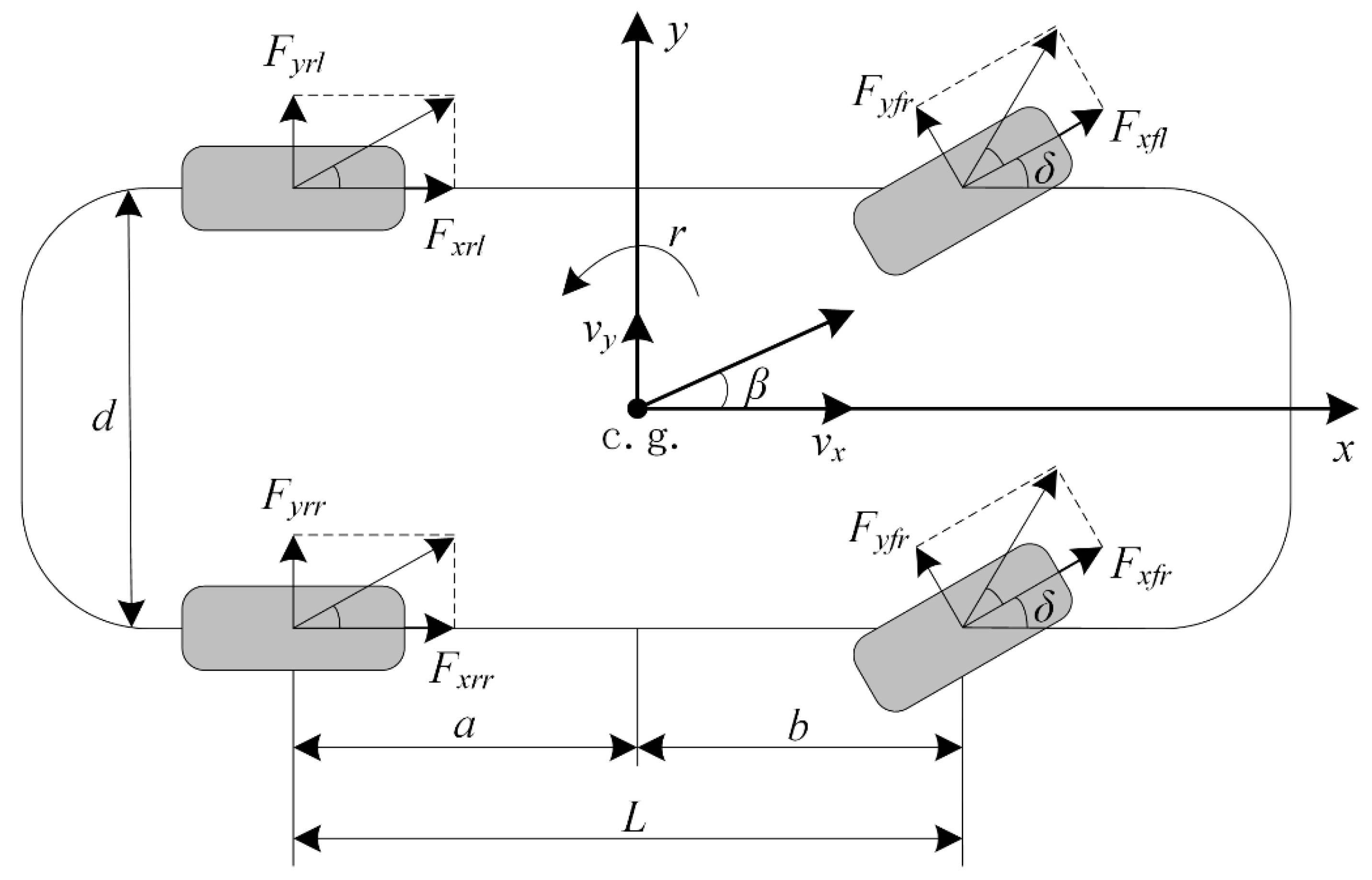
2.2. Seven Degrees of the Freedom Bus Model

Figure 2 is the coordinate system and force analysis of the vehicle. A nonlinear seven-DOF model is set up. The seven degrees of freedom include the movement along the x-axis, movement along the y-axis, rotation around the z-axis, and rotation of the four wheels around their respective axes.

For convenience in the design, this 7-DOF model requires some assumptions:

(1)

The front and rear tires are identical.

(2)

The front steering wheel angles of both sides are the same when the vehicle is turning.

(3)

The influence of elastic damping on the transmission system is not considered.

(4)

The influence of factors such as torsional vibration and shimmy vibration are not considered.

(5)

The influence of the road slope is not considered.

(6)

The road surface is flat and has no influence on the vertical movement of the wheels. The wheel movement caused by the dynamic load on the road surface is ignored.

The dynamic equation is as follows:

$$\left\{\begin{array}{c}m\left({\dot{v}}_x-v_{y}r\right)=\left(F_{xfl}+F_{xfr}\right)cos\delta -\left(F_{yfl}+F_{yfr}\right)sin\delta +F_{xrl}+F_{xrr}\\ m\left({\dot{v}}_y+v_{x}r\right)=\left(F_{xfl}+F_{xfr}\right)sin\delta +\left(F_{yfl}+F_{yfr}\right)cos\delta +F_{yrl}+F_{yrr}\\ I_Z\dot{r}=a\left(F_{xfl}+F_{xfr}\right)sin\delta +a\left(F_{yfl}+F_{yfr}\right)cos\delta -b\left(F_{yrl}+F_{yrr}\right)\\ -\frac{d}{2}\left(F_{xfl}-F_{xfr}\right)cos\delta +\frac{d}{2}\left(F_{yfl}-F_{yfr}\right)sin\delta -\frac{d}{2}\left(F_{xrl}-F_{xrr}\right)\end{array}\right.$$

(6)

where F_x* is the longitudinal force acting on each wheel and F_y* is the lateral force acting on each wheel.

This paper will utilize this model to design the yaw moment controller to calculate the additional yaw moment.

3. Controller Design

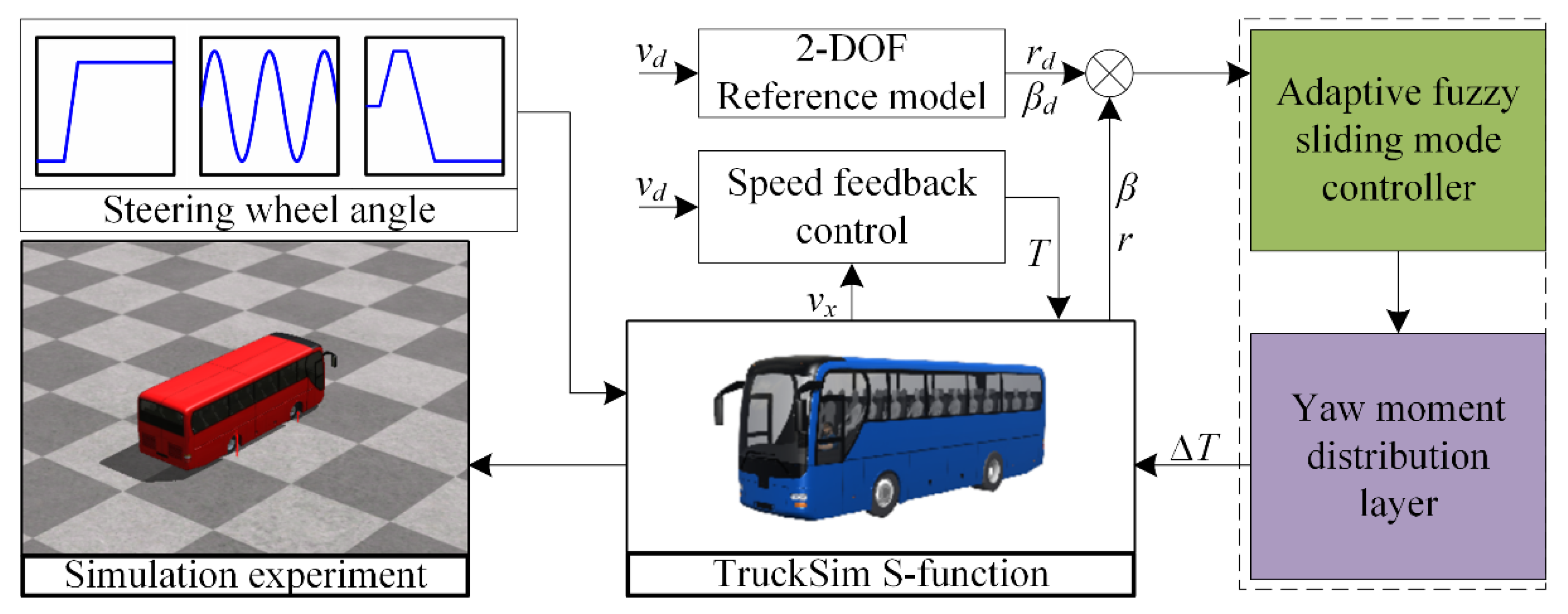
3.1. The Direct Yaw Control Structure of the Bus

Figure 3 displays the main components of the direct yaw control structure. The first is the upper controller that calculates the optimal additional yaw moment. The control method adopted by the upper controller must ensure that the motion state parameters of the bus can follow the ideal value of the reference model under high-speed sharp turns and other situations. The additional yaw moment obtained by the upper controller needs input to the lower controller. On this basis, the lower controller needs to utilize a reasonable method to distribute the additional torque to the four motors. At the same time, the speed feedback controller calculates the required drive torque of the vehicle. Vehicle models, tire models, and power transmission models all use the models in TruckSim. The 2-DOF vehicle reference model, adaptive fuzzy sliding mode controller, torque distribution controller, and other controller structures are designed with Simulink.

3.2. Adaptive Fuzzy Sliding Mode Controller

This article poses the AFSMC method to reduce the instability and disturbance of the steering stability control system of the bus. Usually, the coefficient of the sliding mode surface function cannot be changed after it is determined, and this means that the vehicle status parameters cannot follow the reference value well. Moreover, the traditional SMC does not consider the weight factor between the sideslip angle and the yaw angle in different situations in real time, which makes it difficult to meet the actual needs. Consequently, this paper applies the AFSMC method to change the weight coefficient of the coupling relationship between the sideslip angle and yaw rate adaptively to improve the performance of the dynamic control system.

3.2.1. Sliding Mode Controller

The first step in designing a sliding mode controller is to determine the sliding mode surface function. The choice of the sliding mode surface function is related to the accuracy of the control system. According to the actual needs, this paper designs the sliding mode surface function as:

$$s=k_{1}e+k_2\dot{e}$$

(7)

where k₁ and k₂ are positive constants, k₁ > 0, k₂ > 0. e is the linear sum of the sideslip angle error and yaw angle error, which is defined as the system tracking error:

$$\begin{array}{ll}e& =\lambda e_{\beta }+\left(1-\lambda \right)e_{\phi }\\ & =\lambda \left(\beta -{\beta }_d\right)+\left(1-\lambda \right)\left(\phi -{\phi }_d\right)\end{array}$$

(8)

where φ is the yaw angle and φ_d is the desired yaw angle. λ represents the control weight factor between the sideslip angle and yaw rate, 0 < λ < 1.

The first-order derivation and the second-order derivation of the system tracking error e are obtained:

$$\{\begin{array}{l}\dot{e}=\lambda \left(\dot{\beta }-{\dot{\beta }}_d\right)+\left(1-\lambda \right)\left(r-r_d\right)\\ \ddot{e}=\lambda \left(\ddot{\beta }-{\ddot{\beta }}_d\right)+\left(1-\lambda \right)\left(\dot{r}-{\dot{r}}_d\right)\end{array}$$

(9)

Thus, the derivative of the sliding mode surface function can be obtained as the following formula:

$$\begin{array}{ll}\dot{s}& =k_1\dot{e}+k_2\ddot{e}\\ & =k_1\dot{e}+k_2\left[\lambda \left(\ddot{\beta }-\ddot{\beta }\right)+\left(1-\lambda \right)\left(\dot{r}-{\dot{r}}_d\right)\right]\end{array}$$

(10)

Add the additional yaw moment M_zc to the balance equation of the yaw motion of Equation (6):

$$\dot{r}=\frac{1}{I_Z}\left[M_{zc}+P\right]$$

(11)

where P is expressed as:

$$\begin{array}{c}P=a\left(F_{xfl}+F_{xfr}\right)\sin \delta +a\left(F_{yfl}+F_{yfr}\right)\cos \delta -b\left(F_{yrl}+F_{yrr}\right)\\ -\frac{d}{2}\left(F_{xfl}-F_{xfr}\right)\cos \delta +\frac{d}{2}\left(F_{yfl}-F_{yfr}\right)\sin \delta -\frac{d}{2}\left(F_{xrl}-F_{xrr}\right)\end{array}$$

(12)

Substituting Equation (11) into Equation (10) and making Equation (10) equal to zero:

$$k_1\dot{e}+k_2\{\lambda (\ddot{\beta }-{\ddot{\beta }}_d)+(1-\lambda )[\frac{1}{I_Z}\left(M_{zc}+P\right)-{\dot{r}}_d]\}=0$$

(13)

To satisfy Equation (13), the equivalent control law of AFSMC is shown as:

$$M_{eq}=\frac{I_Z}{1-\lambda }[-\frac{k_1}{k_2}\dot{e}-\lambda (\ddot{\beta }-{\ddot{\beta }}_d)+\left(1-\lambda \right){\dot{r}}_d]-P$$

(14)

The selection principle of the approaching law is to make the system state points that ar far from the sliding mode surface have a larger approaching speed. As a result of this, the system can converge quickly. However, a too large approaching speed will cause the chattering problem in the system.

According to the empirical formula, the following formula is selected as the reaching law function:

$$M_{saw}=\frac{I_Z}{1-\lambda }\left[-\eta sgn\left(s\right)\right]$$

(15)

where η is thee positive constant, η > 0.

The final control law of AFSMC can be obtained:

$$M_{zc}=M_{eq}+M_{saw}=\frac{I_Z}{1-\lambda }\left[-\frac{k_1}{k_2}\dot{e}-\lambda \left(\ddot{\beta }-{\ddot{\beta }}_d\right)+\left(1-\lambda \right){\dot{r}}_d-\eta sgn\left(s\right)\right]-P$$

(16)

The process of proving the stability of the control system based on the Lyapunov stability theory is as follows. According to the definition of the Lyapunov function:

$$V=\frac{1}{2}{s}^2$$

(17)

The formula is obtained by deriving it with respect to time:

$$\dot{V}=s\dot{s}$$

(18)

Substituting Equation (10) into Equation (18) and then substituting Equation (11) into:

$$\dot{V}=s\{k_{1}e+k_2\{\lambda (\ddot{\beta }-{\ddot{\beta }}_d)+\left(1-\lambda \right)[\frac{1}{I_Z}\left(M_{zc}+P\right)-{\dot{r}}_d]\}\}$$

(19)

Substituting Equation (16) into Equation (19), finally the value is obtained:

$$\dot{V}=s\left[-\eta sgn\left(s\right)\right]=-\eta \left|s\right|\le 0$$

(20)

According to the above proof, the system state can eventually converge along the sliding mode surface, and the designed controller will eventually tend to be stable.

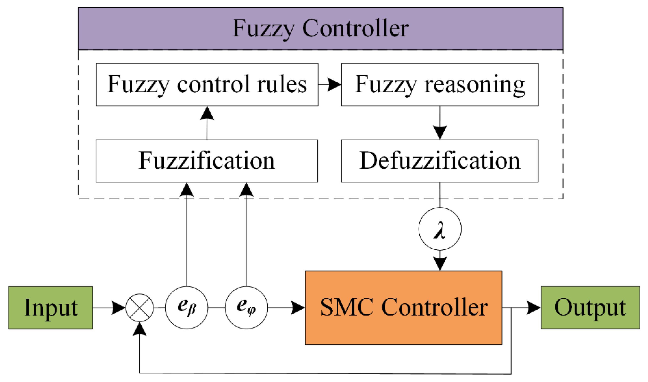
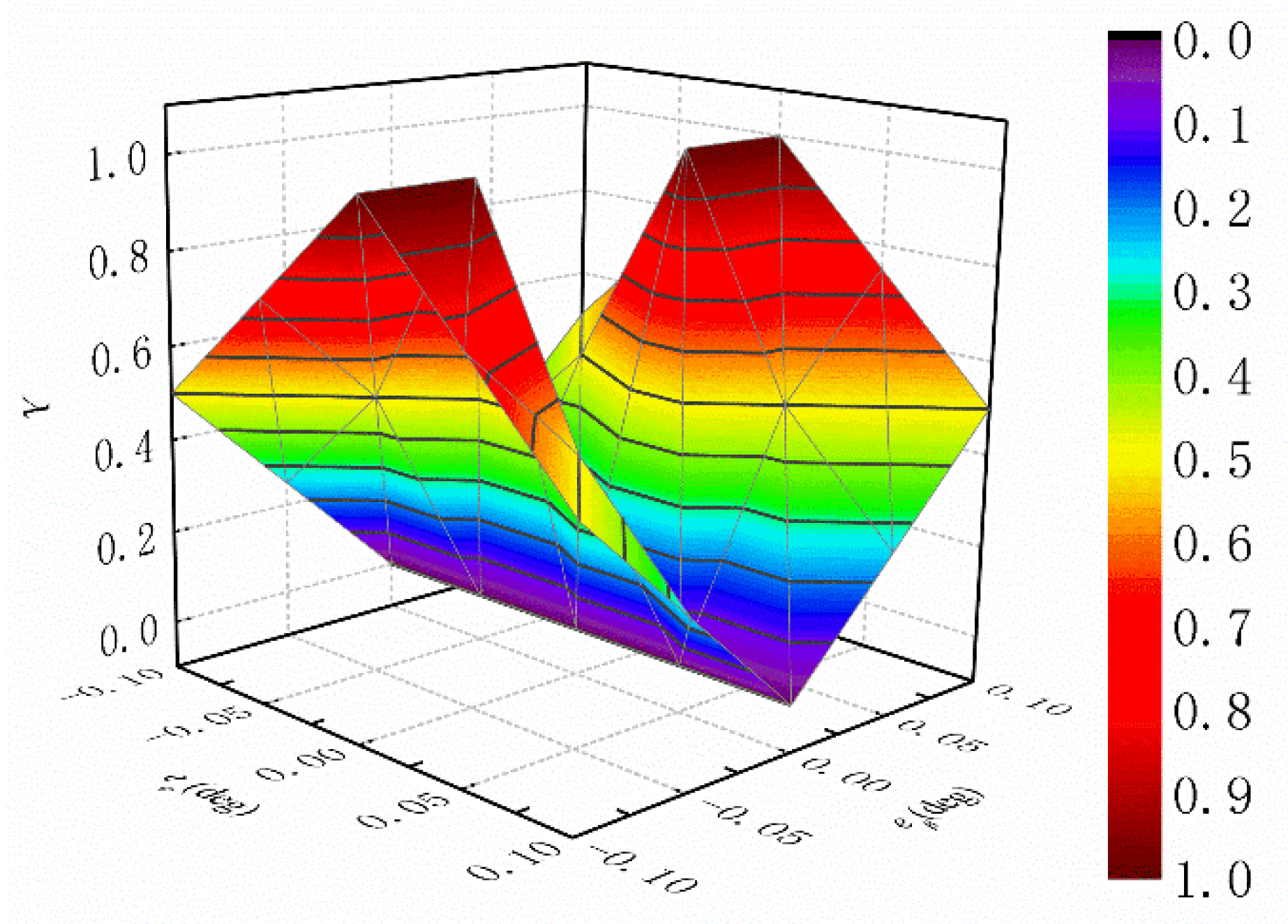
3.2.2. Fuzzy Controller

In this section, we utilize the designed sliding mode surface function to jointly control the sideslip angle and yaw rate. The weighting coefficients of e_β and e_φ are constant, which cannot meet the different requirements of the bus in the actual situation. The weight coefficient λ should be able to be adjusted adaptively according to the vehicle dynamics state. The sliding mode control system has high adaptability. Therefore, fuzzy control is adopted to adjust the weight coefficient λ.

Fuzzy control is a nonlinear control method without an accurate mathematical model. The fuzzy controller fuzzifies the input variables, and fuzzy reasoning is performed on the input variables after fuzzification through fuzzy control rules. Finally, the output variables are obtained after defuzzification processing. Figure 4 displays the structure diagram of the fuzzy controller.

This section designs a fuzzy controller that takes the tracking error of the yaw angle and sideslip angle as the input variables and the weight coefficient λ as the output variable, and sets up five linguistic variables to describe the fuzzification process. They are NB (negative big), NS (negative small), ZO (zero), PS (positive small), and PB (positive big). The designed corresponding fuzzy rules are shown in

Table 2. The fuzzy control rules.

λ	eβ
		NB	NS	ZO	PS	PB
eφ	NB	ZO	PS	PB	PS	ZO
	NS	NS	ZO	PB	ZO	NS
	ZO	NB	NB	NB	NB	NB
	PS	NS	ZO	PB	ZO	NS
	PB	ZO	PS	PB	PS	ZO

.

The quantitative domain of the input and output variables of the fuzzy control system are defined as follows:

(1)

The quantitative domain of the tracking error of the sideslip angle is e_β = {−0.1, −0.05, 0, 0.05, 0.1}.

(2)

The quantitative domain of the tracking error of the yaw angle is e_φ = {−0.1, −0.05, 0, 0.05, 0.1}.

(3)

The quantitative domain of the weight coefficient is λ = {0, 0.25, 0.5, 0.75, 1}.

The three-dimensional surface of the fuzzy control output variables λ is shown in Figure 5.

3.3. Torque Distribution Controller

The additional yaw moment calculated by the AFSMC controller requires a reasonable distribution method. There is dynamic load transfer based on the longitudinal and lateral acceleration when the bus is driving, especially during turning. The maximum longitudinal force on the tire is directly related to the road adhesion coefficient and vertical force.

Therefore, this paper proposes a torque distribution strategy based on the dynamic load proportion in the vertical direction of the wheel. Tire vertical forces are not equal, and the greater the vertical force, the greater the required torque applied to the wheels, and vice versa. The longitudinal force obtained from the AFSMC controller can be distributed in light of the vertical load proportion of each wheel. Under the circumstances, the longitudinal force of each wheel can be effectively utilized.

Based on the statements, it can suppose that:

$$\{\begin{array}{c}\frac{F_{xfl}}{F_{xrl}}=c_l\\ \frac{F_{xfr}}{F_{xrr}}=c_r\end{array}$$

(21)

where c_l and c_r are the ratio of the vertical load on the left and right wheel. Their definitions are as follows:

$$\{\begin{array}{c}{c}_l=\frac{F_{zfl}}{F_{zrl}}\\ c_r=\frac{F_{zfr}}{F_{zrr}}\end{array}$$

(22)

The direct yaw moment and total longitudinal force of the vehicle are:

$$\{\begin{array}{c}{M}_{zc}=\frac{d}{2}\left(F_{xfr}-F_{xfl}\right)\cos \delta +\frac{d}{2}\left(F_{xrr}-F_{xrl}\right)\\ F_x=F_{xfl}\cos \delta +F_{xfr}\cos \delta +F_{xrl}+F_{xrr}\end{array}$$

(23)

Combined with Equations (21) and (23), we can obtain the longitudinal force of each wheel:

$$\{\begin{array}{c}{F}_{xfl}=\frac{1}{\cos \delta +\frac{1}{c_l}}\left(\frac{F_x}{2}-\frac{M_{zc}}{d}\right)\\ F_{xfr}=\frac{1}{\cos \delta +\frac{1}{c_r}}\left(\frac{F_x}{2}+\frac{M_{zc}}{d}\right)\\ F_{xrl}=\frac{1}{c_l\cos \delta +1}\left(\frac{F_x}{2}-\frac{M_{zc}}{d}\right)\\ F_{xrr}=\frac{1}{c_r\cos \delta +1}\left(\frac{F_x}{2}+\frac{M_{zc}}{d}\right)\end{array}$$

(24)

Then, the additional torque of each wheel can be obtained multiplied by the wheel radius. Finally, the resulting values are imported into the TruckSim model.

4. Simulation Results and Discussions

In this section, joint simulation tests of TruckSim and Simulink are performed to verify the effectiveness of AFSMC under a variety of working conditions. Then, we compare the control effect of the AFSMC method with the traditional SMC method. The simulation conditions are: the bus is simulated and tested on flat land of 1 km², regardless of the influence of air resistance, slope resistance, etc., and only the road friction resistance is considered. The bus initial speed v_d is 80 km/h and the road adhesion coefficient μ is 0.85. The rolling resistance coefficient is 1. The simulation time is 10 s. The block diagram of the simulation test flow is shown in Figure 6.

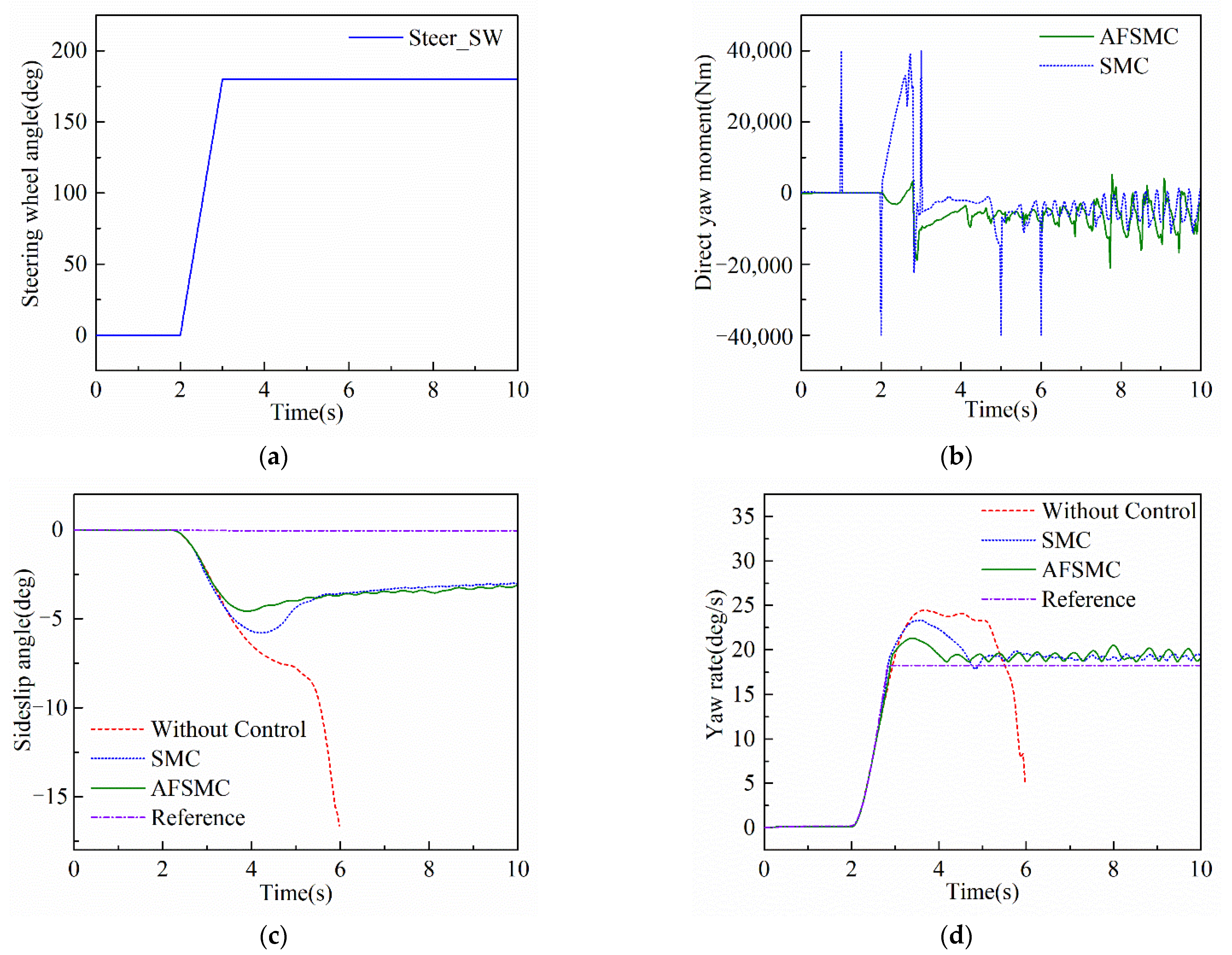
4.1. Step Response Test

The steering wheel angle is input in a step form at a certain vehicle speed. The response characteristics of the vehicle are evaluated with parameters, such as the yaw rate and sideslip angle of the center of mass.

Figure 7a shows that the steering wheel angle increases from 0 to 180 deg in 1 s. As shown in Figure 7b, the value of the traditional SMC method shows many sudden changes. The value of the yaw moment changes drastically from the 2nd second to 3rd second, increasing from 0 to around 40,000 Nm. This may be because the traditional SMC method is sensitive to disturbances before reaching the sliding surface. When the vehicle turns, a large transient abrupt change occurs. On the contrary, the AFSMC method does not have a sudden change. The change in the yaw moment is not so drastic and more stable from the second second to the third second. The AFSMC method is more conducive for the stability of the bus during the steering process.

The sideslip angle and yaw rate of the bus are shown in Figure 7c,d. Uncontrolled vehicles lose stability after the fifth second. The AFSMC method and the SMC method finally reach stability. The sideslip angle is maintained at about −3 deg, and the yaw rate is maintained at about 19 deg. The AFSMC method and SMC method achieve the control purpose. Compared with the SMC method, the AFSMC method has a faster response speed and achieves system stability earlier. The peak values of the yaw rate and sideslip angle are smaller. The peak values of the yaw rate and sideslip angle decreased by 8.62% and 20.90%, respectively, as shown in

Table 3. The peak valve of the sideslip angle and yaw rate under different simulation tests.

Parameter	Simulation Test	SMC	AFSMC	Reduce
Sideslip angle (deg)	Step	5.79	4.58	20.90%
	Sine wave	5.41	4.72	12.75%
	Fishhook	6.17	4.71	23.67%
Yaw rate (deg/s)	Step	23.33	21.32	8.62%
	Sine wave	22.51	20.96	6.89%
	Fishhook	23.61	21.42	9.28%

. They reflect the superiority of the proposed AFSMC method.

From the simulation results of the step response test, we conclude that the AFSMC method can improve the sudden change in the yaw moment during the steering process of the vehicle. It not only prevents the occurrence of dangerous situations, such as instability during vehicle steering, but also effectively reduces the peak value of the sideslip angle and yaw rate.

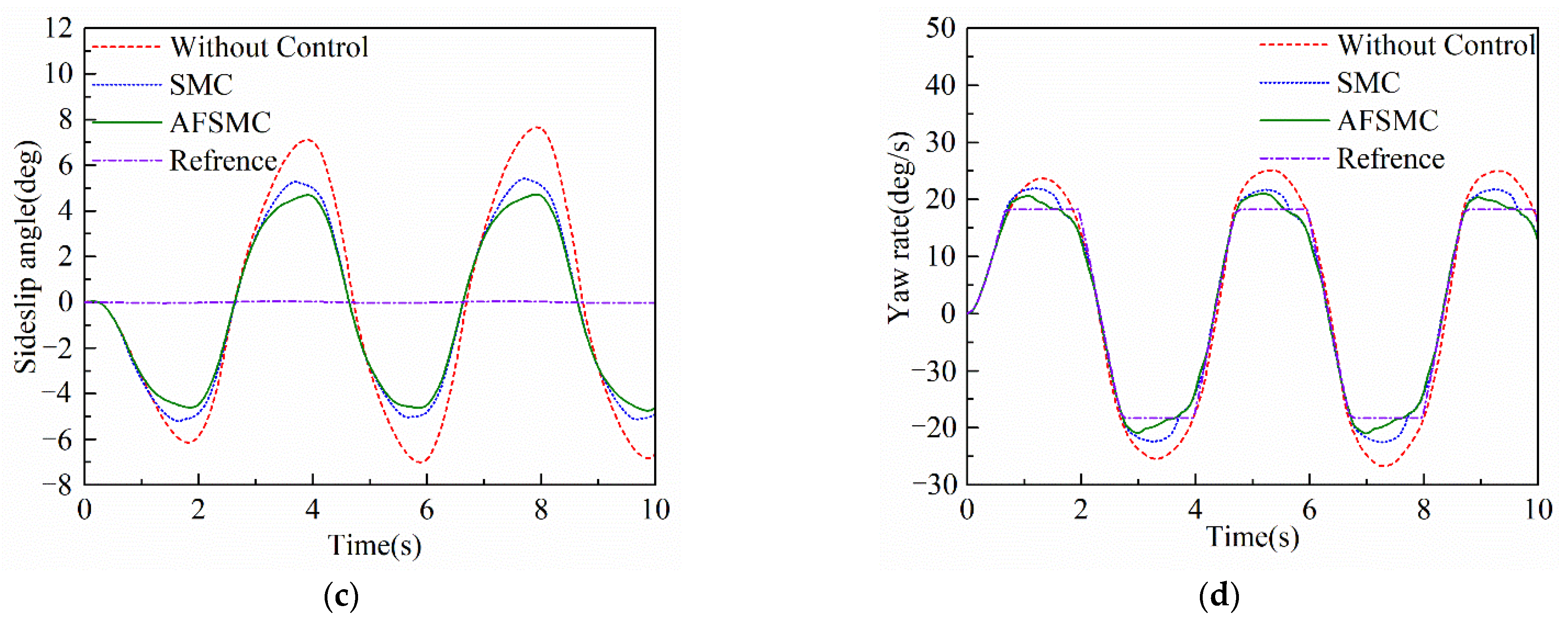
4.2. Sine Wave Response Test

The sine wave test is a commonly used test method to test the stability of the vehicle steering control system. As shown in Figure 8a, the steering wheel angle is the sine wave.

Comparing the additional yaw moment in Figure 8b, the SMC method has sudden changes in many places, for example, at the first second, third second, and fifth second. This may be because when the bus is turning, the motion state changes drastically. Once the traditional SMC is designed, the coefficient cannot be changed. The SMC method cannot adjust the switching gain in real time. It is very sensitive to changes, leading to multiple mutations. Although there is still a small amount of the chattering phenomenon of the additional yaw moment when the AFSMC method is adopted, the chattering amplitude is significantly reduced. Furthermore, the sudden change phenomenon basically disappears, and the yaw moment value changes more smoothly.

As shown in Figure 8c, a bus using the AFSMC method can control the sideslip angle between −4.75 and +4.72 deg. Compared with the uncontrolled bus and SMC method, the dynamic performance is greatly improved. Although the SMC method also has a control effect, the peak value of the sideslip angle controlled by AFSMC is 12.75% lower than SMC shown in Table 3. As shown in Figure 8d, AFSMC has a better response speed. Moreover, Table 3 demonstrates that the peak value of the yaw rate is 6.89% smaller than the SMC methods, which is closer to the ideal value. The AFSMC method has a better control effect than the SMC method.

It can be concluded from the sine wave response test that the AFSMC method can reduce the peak value of the sideslip angle and yaw rate, which can be controlled within a relatively small value during the entire steering process. The sudden changes in the value of the yaw moment are also improved, which can reduce the impact on the motor and is beneficial to prolonging the life of the motor.

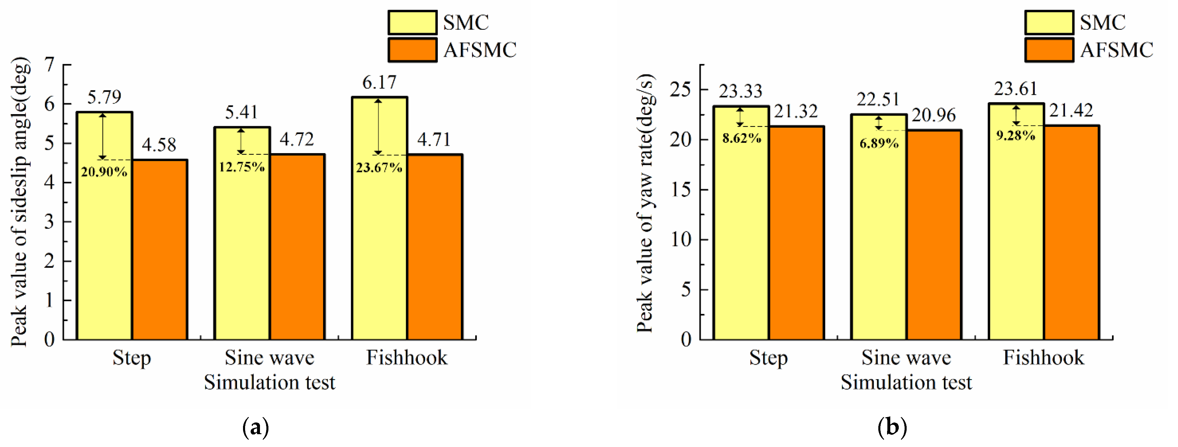
4.3. Fishhook Response Test

The fishhook response test is commonly used to test the stability of a vehicle. It is used to evaluate the safety in a rollover test. Figure 9a shows the steering wheel angle input.

The additional yaw moment obtained by the AFSMC and SMC methods is shown in Figure 9b. The SMC method has many numerical sudden changes. As opposed to this, the AFSMC method does not. Although the additional yaw moment utilizing the AFSMC method shows a chattering phenomenon from the 6th second to 10th second, the chattering amplitude of it is significantly reduced compared with the SMC method. The change in the additional yaw moment value of the AFSMC method is smoother from the beginning to the end. Since the system will adjust the weight coefficient according to the vehicle’s motion state, when the instability trend is large, the follow-up control can be completed by actively adjusting the coefficient.

Figure 9c shows that the sideslip angle of the bus can be limited between −4.71 and +3.51 deg using the AFSMC method. According to the curve in the figure, the uncontrolled vehicle lost stability and oversteered after the eighth second, causing the bus to deviate from the trajectory and even roll over. Although the SMC method also has a control effect, the peak value of the sideslip angle controlled by the AFSMC method decreased more significantly. As shown in Table 3, the peak value of the sideslip angle of the AFSMC method is 23.67% lower than that of the SMC method. We can conclude that the AFSM method has a better control effect than the SMC method in terms of the yaw rate in Figure 9d. Table 3 shows that the peak value of the yaw rate controlled by the AFSMC method is reduced by 9.28% compared to SMC. This method also has a better response speed compared to other methods.

It can be found from the fishhook response test that the proposed AFSMC strategy in this paper controls the value of the sideslip angle and yaw rate within a smaller range by applying a more appropriate yaw moment. The number of sudden changes in the yaw moment value is also significantly reduced. The AFSMC method not only prevents the bus from turning over, but also improves the stability of the bus during the steering process compared to the SMC method.

The peak value of the sideslip angle and yaw rate obtained by the step test, the sine wave test, and the fishhook test were analyzed. The analysis results are shown in Figure 10. Compared with the SMC method, the peak values of the sideslip angle controlled by the AFSMC method are reduced by 20.90%, 12.75%, and 23.67%, respectively, under the three different simulation tests. The peak values of the yaw rate are reduced by 8.62%, 6.89%, and 9.28%, respectively. The peak values are reduced under different operating conditions, which shows the effectiveness of the proposed AFSMC method.

5. Conclusions

This paper proposes an AFSMC method to perfect the driving stability of the bus, and the simulation results verified the effectiveness. The controller has a new sliding mode surface function, and adaptively controls its weight coefficients through the fuzzy algorithm. To distribute the additional yaw moment reasonably, the distribution method according to the vertical load proportion was adopted in this paper.

Through co-simulation analysis by TruckSim and Simulink, the simulation tests were implemented to verify the effectiveness of the proposed AFSMC method. The peak value of the sideslip angle controlled by the AFSMC method was 12.75~23.67% lower than that of the SMC method. The peak value of the yaw rate was 6.89~9.28% lower. At the same time, AFSMC also reduced the serious chattering problems that exist in traditional sliding mode control. Therefore, this method demonstrates a good control effect, which has considerable reference significance for the yaw stability control of a distributed drive electric bus.

The fuzzy rules and membership functions are completely based on experience. The accuracy of the system is not guaranteed. Hence, the weight coefficient of the sideslip angle and yaw rate is not accurate enough under extreme conditions, which is the key problem to be solved in the future work.

References

1. Lin, C.-L.; Hung, H.-C.; Li, J.-C. Active control of regenerative brake for electric vehicles. Actuators 2018, 7, 84. [Google Scholar] [CrossRef] [Green Version]
2. Sun, P.; Stensson Trigell, A.; Drugge, L.; Jerrelind, J. Energy-efficient direct yaw moment control for in-wheel motor electric vehicles utilising motor efficiency maps. Energies 2020, 13, 593. [Google Scholar] [CrossRef] [Green Version]
3. Wang, H.; Sun, Y.; Gao, Z.; Chen, L. Extension coordinated multi-objective adaptive cruise control integrated with direct yaw moment control. Actuators 2021, 10, 295. [Google Scholar] [CrossRef]
4. Ahmadian, N.; Khosravi, A.; Sarhadi, P. Driver assistant yaw stability control via integration of AFS and DYC. Veh. Syst. Dyn. 2021, 1–21. [Google Scholar] [CrossRef]
5. Chen, T.; Chen, L.; Xu, X.; Cai, Y.; Jiang, H.; Sun, X. Passive fault-tolerant path following control of autonomous distributed drive electric vehicle considering steering system fault. Mech. Syst. Signal Processing 2019, 123, 298–315. [Google Scholar] [CrossRef]
6. Chen, T.; Xu, X.; Chen, L.; Jiang, H.; Cai, Y.; Li, Y. Estimation of longitudinal force, lateral vehicle speed and yaw rate for four-wheel independent driven electric vehicles. Mech. Syst. Signal Processing 2018, 101, 377–388. [Google Scholar] [CrossRef]
7. Guo, J.; Luo, Y.; Li, K.; Dai, Y. Coordinated path-following and direct yaw-moment control of autonomous electric vehicles with sideslip angle estimation. Mech. Syst. Signal Processing 2018, 105, 183–199. [Google Scholar] [CrossRef]
8. Zhang, J.; Zhou, S.; Li, F.; Zhao, J. Integrated nonlinear robust adaptive control for active front steering and direct yaw moment control systems with uncertainty observer. Trans. Inst. Meas. Control. 2020, 42, 3267–3280. [Google Scholar] [CrossRef]
9. Liu, W.; Khajepour, A.; He, H.; Wang, H.; Huang, Y. Integrated torque vectoring control for a three-axle electric bus based on holistic cornering control method. IEEE Trans. Veh. Technol. 2018, 67, 2921–2933. [Google Scholar] [CrossRef]
10. Zhu, H.; Li, L.; Jin, M.; Li, H.; Song, J. Real-time yaw rate prediction based on a non-linear model and feedback compensation for vehicle dynamics control. Proc. Inst. Mech. Eng. Part D J. Automob. Eng. 2013, 227, 1431–1445. [Google Scholar] [CrossRef]
11. Yu, Z.; Leng, B.; Xiong, L.; Feng, Y.; Shi, F. Direct yaw moment control for distributed drive electric vehicle handling performance improvement. Chin. J. Mech. Eng. 2016, 29, 486–497. [Google Scholar] [CrossRef]
12. Huang, W.; Wong, P.K.; Wong, K.I.; Vong, C.M.; Zhao, J. Adaptive neural control of vehicle yaw stability with active front steering using an improved random projection neural network. Veh. Syst. Dyn. 2019, 59, 396–414. [Google Scholar] [CrossRef]
13. Swain, S.K.; Rath, J.J.; Veluvolu, K.C. Neural network based robust lateral control for an autonomous vehicle. Electronics 2021, 10, 510. [Google Scholar] [CrossRef]
14. Li, B.; Du, H.; Li, W.; Zhang, B. Non-linear tyre model–based non-singular terminal sliding mode observer for vehicle velocity and side-slip angle estimation. Proc. Inst. Mech. Eng. Part D J. Automob. Eng. 2018, 233, 38–54. [Google Scholar] [CrossRef] [Green Version]
15. Li, Z.; Wang, P.; Liu, H.; Hu, Y.; Chen, H. Coordinated longitudinal and lateral vehicle stability control based on the combined-slip tire model in the MPC framework. Mech. Syst. Signal Processing 2021, 161, 107947. [Google Scholar] [CrossRef]
16. Liu, H.; Yan, S.; Shen, Y.; Li, C.; Zhang, Y.; Hussain, F. Model predictive control system based on direct yaw moment control for 4WID self-steering agriculture vehicle. Int. J. Agric. Biol. Eng. 2021, 14, 175–181. [Google Scholar] [CrossRef]
17. Shi, K.; Yuan, X.; Huang, G.; He, Q. MPC-based compensation control system for the yaw stability of distributed drive electric vehicle. Int. J. Syst. Sci. 2018, 49, 1795–1808. [Google Scholar] [CrossRef]
18. Hou, R.; Zhai, L.; Sun, T.; Hou, Y.; Hu, G. Steering stability control of a four in-wheel motor drive electric vehicle on a road with varying adhesion coefficient. IEEE Access 2019, 7, 32617–32627. [Google Scholar] [CrossRef]
19. Kim, J.; Park, C.; Hwang, S.; Hori, Y.; Kim, H. Control algorithm for an independent motor-drive vehicle. IEEE Trans. Veh. Technol. 2010, 59, 3213–3222. [Google Scholar] [CrossRef]
20. Ding, S.; Liu, L.; Zheng, W.X. Sliding mode direct yaw-moment control design for in-wheel electric vehicles. IEEE Trans. Ind. Electron. 2017, 64, 6752–6762. [Google Scholar] [CrossRef]
21. Tota, A.; Lenzo, B.; Lu, Q. On the experimental analysis of integral sliding modes for yaw rate and sideslip control of an electric vehicle with multiple motors. Int. J. Automot. Technol. 2018, 19, 811–823. [Google Scholar] [CrossRef]
22. Guo, N.; Zhang, X.; Zou, Y.; Lenzo, B.; Du, G.; Zhang, T. A supervisory control strategy of distributed drive electric vehicles for coordinating handling, lateral stability, and energy efficiency. IEEE Trans. Transp. Electrif. 2021, 7, 2488–2504. [Google Scholar] [CrossRef]
23. Mousavinejad, E.; Han, Q.-L.; Yang, F.; Zhu, Y.; Vlacic, L. Integrated control of ground vehicles dynamics via advanced terminal sliding mode control. Veh. Syst. Dyn. 2016, 55, 268–294. [Google Scholar] [CrossRef]
24. Du, L.; Ji, J.; Zhang, D.; Zheng, H.; Chen, W. A fuzzy drive strategy for an intelligent vehicle controller unit integrated with connected data. Machines 2021, 9, 215. [Google Scholar] [CrossRef]
25. Zhang, S.; Chen, Y.; Zhang, W. Spatiotemporal fuzzy-graph convolutional network model with dynamic feature encoding for traffic forecasting. Knowl. Based Syst. 2021, 231, 107403. [Google Scholar] [CrossRef]
26. Pu, Z.; Cui, Z.; Tang, J.; Wang, S.; Wang, Y. Multi-modal traffic speed monitoring: A real-time system based on passive Wi-Fi and bluetooth sensing technology. IEEE Internet Things J. 2021, 1-1. [Google Scholar] [CrossRef]
27. Qi, W.; Maseleno, A.; Yuan, X.; Balas, V.E. Fuzzy control strategy of pure electric vehicle based on driving intention recognition. J. Intell. Fuzzy Syst. 2020, 39, 5131–5139. [Google Scholar] [CrossRef]
28. Sun, X.; Wang, Y.; Cai, Y.; Wong, P.K.; Chen, L. An adaptive nonsingular fast terminal sliding mode control for yaw stability control of bus based on STI tire model. Chin. J. Mech. Eng. 2021, 34, 1–14. [Google Scholar] [CrossRef]
29. Asiabar, A.N.; Kazemi, R. A direct yaw moment controller for a four in-wheel motor drive electric vehicle using adaptive sliding mode control. Proc. Inst. Mech. Eng. Part K J. Multi-Body Dyn. 2019, 233, 549–567. [Google Scholar] [CrossRef]
30. Fu, C.; Hoseinnezhad, R.; Li, K.; Hu, M. A novel adaptive sliding mode control approach for electric vehicle direct yaw-moment control. Adv. Mech. Eng. 2018, 10, 1–12. [Google Scholar] [CrossRef] [Green Version]
31. Zhang, H.; Liang, J.; Jiang, H.; Cai, Y.; Xu, X. Stability research of distributed drive electric vehicle by adaptive direct yaw moment control. IEEE Access 2019, 7, 106225–106237. [Google Scholar] [CrossRef]
Figure 1. The 2-DOF distributed drive electric bus model.
Energies 15 01280 g001
Figure 2. The 7-DOF distributed drive electric bus model.
Energies 15 01280 g002
Figure 3. The control structure of the direct yaw moment.
Energies 15 01280 g003
Figure 4. The structure diagram of the fuzzy controller.
Energies 15 01280 g004
Figure 5. The three-dimensional surface of the weight coefficient λ.
Energies 15 01280 g005
Figure 6. The block diagram of the simulation test flow.
Energies 15 01280 g006
Figure 7. The simulation results of the step response test. (a) Steering wheel angle; (b) direct yaw moment; (c) sideslip angle; (d) yaw rate.
Energies 15 01280 g007
Figure 8. The simulation results of the sine wave response test. (a) Steering wheel angle; (b) direct yaw moment; (c) sideslip angle; (d) yaw rate.
Energies 15 01280 g008aEnergies 15 01280 g008b
Figure 9. The simulation results of the fishhook response test. (a) Steering wheel angle; (b) direct yaw moment; (c) sideslip angle; (d) yaw rate.
Energies 15 01280 g009
Figure 10. The peak values under different simulation tests. (a) Sideslip angle; (b) yaw rate.
Energies 15 01280 g010