Influence of Coil Current and Oil Film Thickness on Hopf Bifurcation of MLDSB

Abstract

Magnetic-liquid double-suspension bearing (MLDSB) is composed of an electromagnetic supporting system and a hydrostatic supporting system. Due to its greater supporting capacity and stiffness, it is appropriate for middle-speed applications, overloading, and frequent starting. However, because it contains two sets of systems, its structure and rotor support system are more complex. It contains strong nonlinear links. When the parameters of the system change, the bearing rotor may feature Hopf bifurcation, resulting in system flutter and reducing the operational stability of the magnetic fluid double-suspension bearing rotor, which has become one of the key problems restricting its development and application. As key parameters of MLDSB, the coil current and oil film thickness exert a major impact on Hopf bifurcation. Therefore, the mathematical model of MLDSB is established in this paper, and the border and direction of Hopf bifurcation, period, and amplitude of limit cycle are analyzed. The calculation, simulation, and experimental results show that when the coil current and oil film thickness of the bearing system are greater than the boundary value of the Hopf bifurcation, Hopf bifurcation will occur, resulting in the vibration of the bearing rotor and affecting the stability of the system. In addition, when analyzing the combined effects of coil current and oil film thickness on the Hopf bifurcation of the system, it was found that the boundary value of Hopf bifurcation in the system is reduced compared with when it is are affected solely due to the coupling of the two parameters. The period, amplitude and vibration speed of limit cycle increase with increases in the coil current and oil film thickness. Hopf bifurcation experiment was conducted on MLDSB testing system. The results show that Hopf bifurcation does not occur when i₀ < 0.5 A, the bearing rotor operates stably in the balanced position, i₀ > 1.0 A, Hopf bifurcation occurs in the system, and the bearing rotor vibrates with equal amplitude, which reduces the stability of operation. The research in this paper can provide a theoretical reference for the Hopf bifurcation analysis of MLDSB.

1. Introduction

As a novel supporting system, MLDSB is dominated by electromagnetic suspension and supplemented by hydrostatic support. It offers plenty of advantages, such as a lack of mechanical contact, strong carrying capacity, high stiffness, and so on, which make it appropriate for deep-sea exploration, hydroelectric power generation, and other fields, especially for working in conditions of middle speed, overloading, and frequent starting [1].

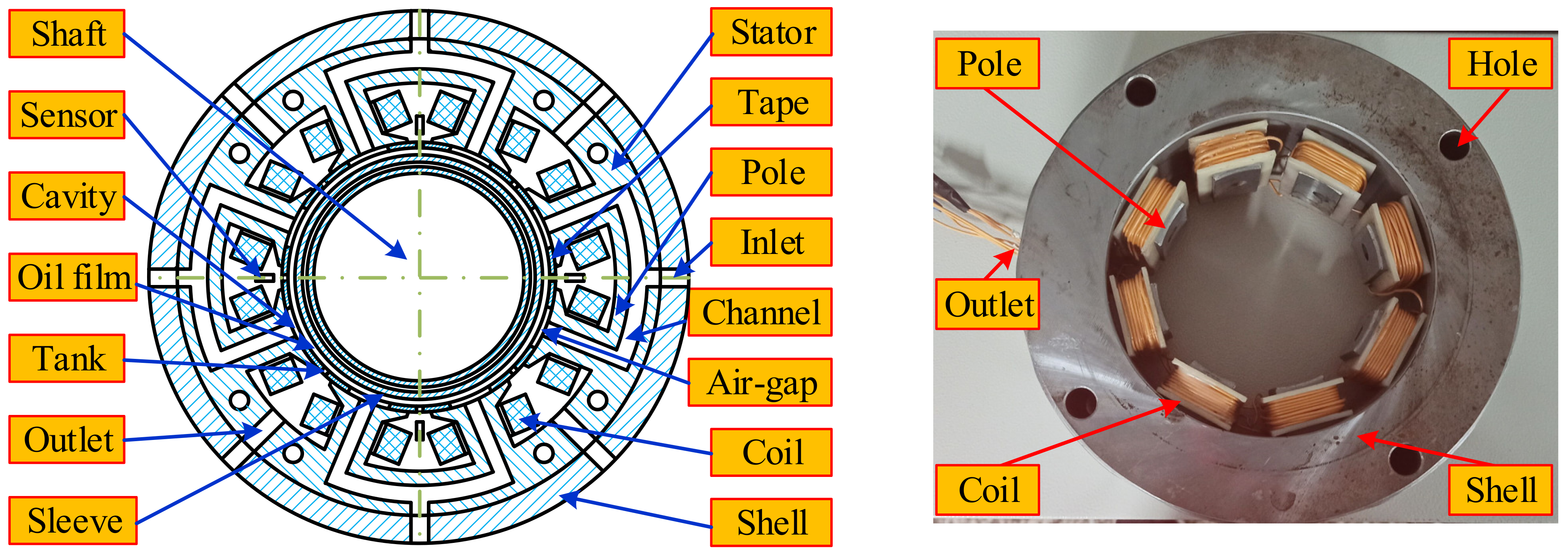
MLDSB includes a bracket, a variable speed motor, coupling, a stepped shaft, journal bearing, axial bearing, an axial loading motor, and a journal motor, as shown in Figure 1.

The radial unit of MLDSB is composed a of step shaft, a magnetic guide sleeve, a supporting cavity, a magnetic pole, an inlet pipe, a shell, a coil, and an outlet, as shown in Figure 2.

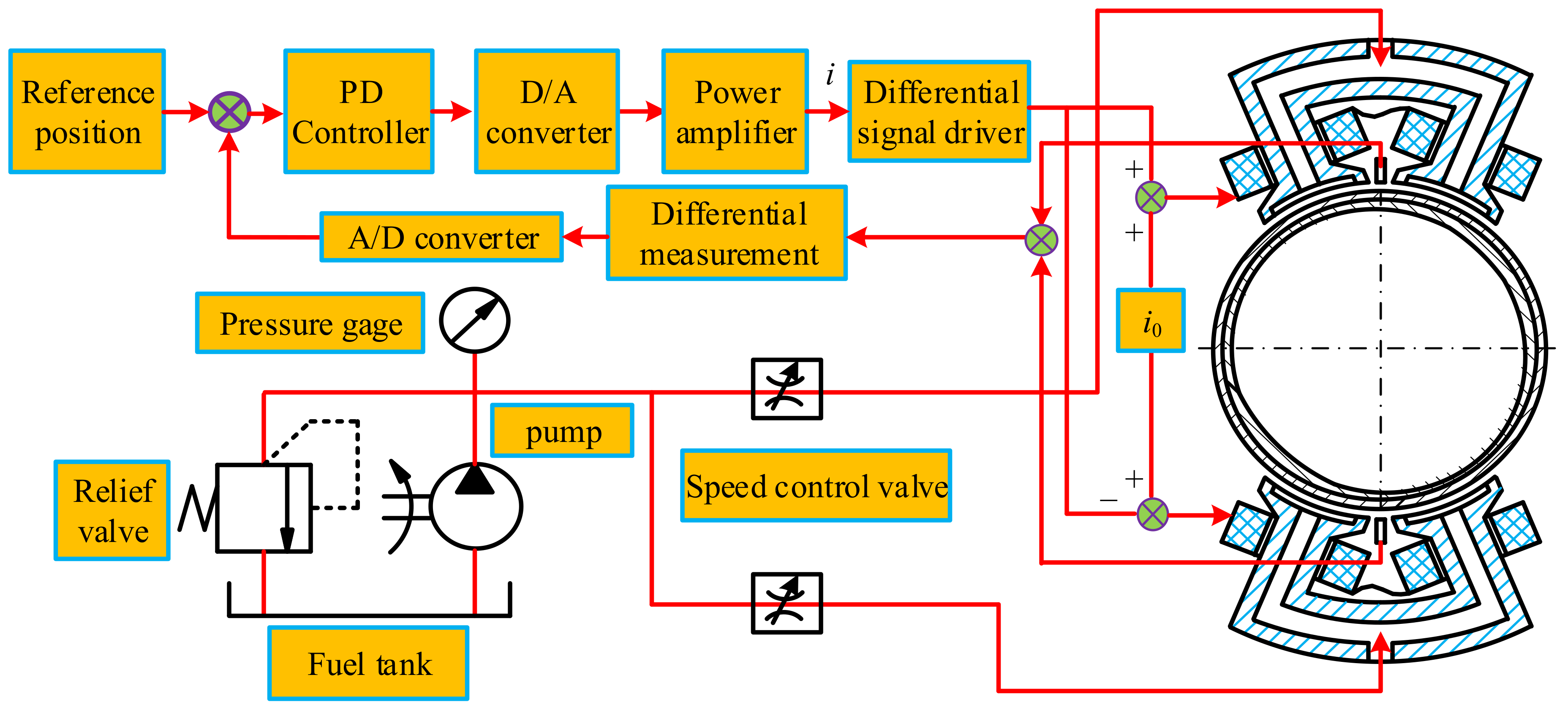
The regulation principle of MLDSB is shown as Figure 3 [2]. Due to its strong nonlinear characteristics and complicated damping characteristics, it features mutual coupling between its two supporting systems, and Hopf bifurcation phenomenon occurs easily; consequently, the reliability and operational stability of MLDSB are reduced.

In recent years, many scholars have studied the Hopf bifurcation behavior of electromagnetic bearings and achieved fruitful results. Hopf bifurcation is a relatively simple and important bifurcation problem in nonlinear dynamic systems. It belongs to local dynamic bifurcation. Specifically, it refers to the phenomenon whereby the system suddenly bifurcates from the equilibrium point to the limit cycle at the non-hyperbolic equilibrium point in response to changes in the bifurcation parameters. It is widely used in the study of the dynamic characteristics of various complex nonlinear dynamic systems. The inherent nonlinear dynamic essence of the system is revealed through Hopf bifurcation, and a corresponding control strategy and optimization method are proposed.

Due to the introduction of hydrostatic force, the rotor force of MLDSB is more complex than that of traditional electromagnetic bearing, so it is difficult to analyze Hopf bifurcation behavior.

As the key parameters in the supporting characteristics of MLDSB, oil film thickness and coil current exert a major impact on Hopf bifurcation behavior. Therefore, this paper intends to establish a mathematical model of the magneto-hydraulic coupling force of MLDSB and to explore the internal influence laws governing the influence oil film thickness and coil current on the Hopf bifurcation boundary, limit cycle period, and phase trajectory of a single-DOF supporting system, so as to provide a theoretical basis for the design and stable operation of MLDSB.

2. Dynamics Model of Single-DOF Supporting System

The dynamics equation for a single-DOF supporting system in MLDSB is as follows [2]:

$$\left\{\begin{array}{l}\dot{x}=y\\ y=-\frac{1}{m}f\left(x,\dot{x}\right)-\frac{1}{m}g\left(x,\dot{x}\right)\end{array}\right.$$

(1)

where $f\left(x,\dot{x}\right)=F_{l0}\dot{x}\left[\frac{1}{{\left(1+\overline{x}\cos \theta \right)}^3}-\frac{1}{{\left(1-\overline{x}\cos \theta \right)}^3}\right]$;

$g\left(x,\dot{x}\right)=F_{e0}\left[{\left(\frac{1-{\overline{i}}_c}{1+\overline{x}\cos \theta }\right)}^2-{\left(\frac{1+{\overline{i}}_c}{1-\overline{x}\cos \theta }\right)}^2\right]-F_{l0}\left[\frac{1}{{\left(1+\overline{x}\cos \theta \right)}^3}-\frac{1}{{\left(1-\overline{x}\cos \theta \right)}^3}\right]$;

${\overline{i}}_c=i_c/i_0$; $\overline{x}=x/h_0$; x is the displacement, y is the velocity, g is the acceleration of gravity, i_c is rthe egulation current, and θ is the included angle of magnetic poles.

The design parameters of MLDSB are shown in

Table 1. Design parameters of MLDSB.

Symbol	Variable	Value
A	Length of Supporting Cavity	0.1 m
A1	Magnetic Area	1000 mm2
Ab	Extrusion area	1056 mm2
Ae	Supporting Area	1504 mm2
B	Width of Supporting Cavity	0.02 m
$\overline{B}$	Flow coefficient	4.3611
Kd	Differential Coefficient	0.05
Kp	Scale Coefficient	−70
N	Turns of Coil	60
a	Length of Sealing Tape	0.006 m
h0	Oil Film Thickness	30 μm
i0	Initial current	2 A
k	Electromagnetic coefficient	2.38 × 10−5
m	Rotor Mass	100 kg
q0	Supporting Cavity Flow	3.2622 L/min
μ	Viscosity	1.307 × 10−3 Pa.s
b	Width of Sealing Tape	0.004 m
μ0	Air Permeability	4π × 10−7 H/m

[3]. The range of coil current i₀ is (0.5, 1.2) A. $\overline{x}$ is the displacement after dimensionless treatment, F_e0 is the initial electromagnetic force, and F_l0 is the initial hydraulic pressure.

3. Influence of Coil Current and Oil Film Thickness on Hopf Bifurcation of MLDSB

3.1. Influence of Coil Current on Hopf Bifurcation of MLDSB

3.1.1. Hopf Bifurcation Boundary

According to Hopf bifurcation theory [4,5,6], the Jacobian matrix of Equation (1) is obtained as follows:

$$\mathit{A}=\left(\begin{array}{cc}0& 1\\ a_{21}& a_{22}\end{array}\right)$$

(2)

$${\lambda }^2-a_{22}\lambda -a_{21}=0$$

(3)

$${\lambda }_{1,2}=\frac{{\alpha }_1}{2}\pm \frac{1}{2}\sqrt{{\alpha }_1^2+4{\beta }_1}$$

(4)

where $a_{21}=\frac{8i_0^{2}k{\cos }^2\theta }{m{h}_0^3}-\frac{6{\delta }_1\cos \theta }{m{h}_0^4}+\frac{1200K_{p}k{i}_0\cos \theta }{m{h}_0^2}$;

$a_{22}=\frac{-2{\delta }_2}{m{h}_0^3}+\frac{1200K_d{i}_{0}k\cos \theta }{m{h}_0^2}$; ${\delta }_1=\frac{2\mu q_0{A}_e\cos \theta }{\overline{B}}$; ${\delta }_2=\frac{2\mu A_e{A}_b{\cos }^2\theta }{\overline{B}}$;

${\alpha }_1=693.31i_0-597.17$; ${\beta }_1=2.83\times {10}^6{i}_0^2-9.71\times {10}^5{i}_0-3.07\times {10}^6$.

According to Equations (2)–(4), the Hopf bifurcation boundary of a single-DOF supporting system is i₀ = 0.86 A. When i₀ > 0.86 A, Hopf bifurcation occurs in the bearing system, resulting in the vibration of the bearing rotor and affecting the stability of operation.

3.1.2. Hopf Bifurcation Direction

Take the partial derivative of both sides of Equation (3) with respect to i₀.

$$\frac{\mathrm{d}\lambda }{\mathrm{d}{i}_0}=\frac{{\epsilon }_1}{{\phi }_1}$$

(5)

where ${\epsilon }_1=\frac{16k\cos \theta i_0}{m{h}_0^3}+\frac{1200k\cos \theta }{m{h}_0^2}\left(K_p+K_d\lambda \right)$;

${\phi }_1=2\lambda +\frac{4\mu A_e{A}_b{\cos }^2\theta }{m\overline{B}{h}_0^3}-\frac{1200K_d{i}_{0}k\cos \theta }{m{h}_0^2}$${\lambda }_{1,2}=-0.46\pm 1.35\times {10}^{3}i$ when i₀ = 0.86 A, and the cross-sectional coefficient can be obtained as follows.

$${\sigma }^{\prime }\left(i_0\right)=Re\left(\frac{d\lambda }{d{i}_0}\left|\begin{array}{c}\\ \\ i_0=0.86\end{array}\right.\right)=346.67$$

(6)

According to Equation (6), supercritical Hopf bifurcation occurs when the cross-sectional coefficient is greater than zero. In other words, when i₀ < 0.86 A, the single-DOF supporting system achieves a stable balance state without Hopf bifurcation. When i₀ > 0.86 A, the phase trajectory is a stable limit cycle and the Hopf bifurcation phenomenon occurs.

3.1.3. Influence of Coil Current on Limit Cycle Period

According to Hopf bifurcation theory, the period of the limit cycle is shown as follows.

$$T=\frac{4\mathsf{\pi }}{\sqrt{-\left({\eta }_1^2+4{\gamma }_1\right)}}$$

(7)

where ${\eta }_1=693.31i_0-597.17$; ${\gamma }_1=2.83\times {10}^6{i}_0^2-9.71\times {10}^5{i}_0-3.07\times {10}^6$.

Substituting the data in Table 1 into Equation (7), the period T of limit cycle can be obtained as shown in Figure 4.

According to Figure 4, the period of the limit cycle increases with the increase in current i₀. When i₀ < 1.1 A, it creates little impact on the period of the limit cycle. When i₀ > 1.1 A, the limit cycle period is greatly affected.

3.2. Influence of Oil Film Thickness on Hopf Bifurcation of MLDSB

3.2.1. Hopf Bifurcation Boundary

Set i₀ = 1.2 A, the root of characteristic equation of Jacobian matrix can be obtained as follows:

$$\frac{{\alpha }_2}{2}\pm \frac{1}{2}\sqrt{{\alpha }_2^2+4{\beta }_2}$$

(8)

where ${\alpha }_2=\frac{7.49\times {10}^{-7}}{h_0^2}-\frac{1.61\times {10}^{-11}}{h_0^3}$; ${\beta }_2=\frac{1.10\times {10}^{-7}}{h_0^3}-\frac{2.49\times {10}^{-12}}{h_0^4}-\frac{1.05\times {10}^{-3}}{h_0^2}$.

According to Equation (8), the bifurcation boundary is h₀ = 2.5 × 10⁻⁵ m.

3.2.2. Hopf Bifurcation Direction

The derivative of bifurcation parameter h₀ on both sides of Equation (3) is obtained as follows.

$$\frac{\mathrm{d}\lambda }{\mathrm{d}{h}_0}=\frac{{\epsilon }_{2,1}+{\epsilon }_{2,2}}{{\phi }_2}$$

(9)

where ${\epsilon }_{2,1}=\frac{{\cos }^2\theta }{m}\left(\frac{-24k{i}_0^2}{h_0^4}+\frac{48\mu q_0{A}_e}{\overline{B}{h}_0^5}-\frac{2400K_{p}k{i}_0}{h_0^3\cos \theta }\right)$; ${\lambda }_{1,2}=84\pm 1003.7i$.

${\epsilon }_{2,2}=\left(\frac{12\mu A_e{A}_b{\cos }^2\theta }{m\overline{B}{h}_0^4}-\frac{2400K_{d}k{i}_0\cos \theta }{m{h}_0^3}\right)\lambda$; ${\phi }_2=2\lambda +\frac{4\mu A_e{A}_b{\cos }^2\theta }{m\overline{B}{h}_0^3}-\frac{1200K_d{i}_{0}k\cos \theta }{m{h}_0^2}$.

When h₀ = 2.5 × 10⁻⁵ m, the cross-sectional coefficient can be obtained as follows.

$${\sigma }^{\prime }\left(h_0\right)=\mathrm{Re}\left({\left.\frac{\mathrm{d}\lambda }{\mathrm{d}{h}_0}\right|}_{h_0=2.5\times {10}^{-5}}\right)=1.34\times {10}^7$$

(10)

According to Equation (10), supercritical Hopf bifurcation occurs when the cross-cutting coefficient is greater than zero. In other words, when h₀ < 2.5 × 10⁻⁵ m, the single-DOF supporting system achieves a stable balance state without Hopf bifurcation. When h₀ > 2.5 × 10⁻⁵ m, the phase trajectory is the stable limit cycle and Hopf bifurcation occurs.

3.2.3. Effect of Oil Film Thickness on Limit Cycle Period

According to Hopf bifurcation theory, the limit cycle period is obtained as follows:

$$T=\frac{4\pi }{\sqrt{-\left({\eta }_2^2+4{\gamma }_2\right)}}$$

(11)

where ${\eta }_2=\frac{7.49\times {10}^{-7}}{h_0^2}-\frac{1.61\times {10}^{-11}}{h_0^3}$; ${\gamma }_2=\frac{1.10\times {10}^{-7}}{h_0^3}-\frac{1.05\times {10}^{-3}}{h_0^2}-\frac{2.49\times {10}^{-12}}{h_0^4}$.

Substituting the data in Table 1 into Equation (11), the period T of limit cycle is obtained, as shown as Figure 5.

According to Figure 5, the period of limit cycle increases with the increase in oil film thickness. When h₀ < 2.8 × 10⁻⁵ m, the oil film thickness exerts little effect on the limit cycle period. When h₀ > 2.8 × 10⁻⁵ m, the limit cycle period is greatly affected.

3.3. Compound Effect of Coil Current and Oil Film Thickness on Hopf Bifurcation of MLDSB

3.3.1. Hopf Bifurcation Boundary

Setting i₀ and h₀ as the variables, the roots of characteristic equation of Jacobian matrix can be obtained as follows.

$$\frac{{\alpha }_3}{2}\pm \frac{1}{2}\sqrt{{\alpha }_3^2+4{\beta }_3}$$

(12)

where ${\alpha }_3=\frac{6.24\times {10}^{-7}{i}_0}{h_0^2}-\frac{1.61\times {10}^{-11}}{h_0^3}$;

${\beta }_3=\frac{7.65\times {10}^{-8}{i}_0^2}{h_0^3}-\frac{2.49\times {10}^{-12}}{h_0^4}-\frac{8.74\times {10}^{-4}{i}_0}{h_0^2}$.

According to Equation (12), the bifurcation boundary curve is obtained as follows.

$$i_0=\frac{h_0^3+1.61\times {10}^{-4}}{6.24h_0}$$

(13)

3.3.2. Hopf Bifurcation Direction

According to Equations (6) and (10), the cross-sectional coefficient is greater than zero; consequently, the Hopf bifurcation direction can be inferred as shown in Figure 6.

According to Figure 6, when the parameters are on the left side of the boundary line, the single-DOF supporting system achieves stable balance without Hopf bifurcation. When the parameters are on the right side (the shaded region), the phase trajectory is the stable limit cycle and Hopf bifurcation phenomenon occurs. When one parameter is small, the stability region of another parameter can be effectively expanded.

3.3.3. Limit Cycle Period

According to Hopf bifurcation theory, the limit cycle period is obtained.

$$T=\frac{4\pi }{\sqrt{-\left({\eta }_3^2+4{\gamma }_3\right)}}$$

(14)

where ${\eta }_3=\frac{6.24\times {10}^{-7}{i}_0}{h_0^2}-\frac{1.61\times {10}^{-11}}{h_0^3}$;

${\gamma }_3=\frac{7.65\times {10}^{-8}{i}_0^2}{h_0^3}-\frac{2.49\times {10}^{-12}}{h_0^4}-\frac{8.74\times {10}^{-4}{i}_0}{h_0^2}$.

Substituting the data in Table 1 into Equation (14), the period T of limit cycle is obtained as follows.

According to Figure 7, the period of limit cycle increases with the increase in coil current and oil film thickness. The oil film thickness exerts little effect on the limit cycle period when the coil current and oil film thickness are small, and the limit cycle period is greatly affected while larger.

4. Simulation and Experiment

When the phase trajectory becomes a limit cycle, Hopf bifurcation occurs; subsequently, the oscillation degree can be reflected by the amplitude and maximum vibration velocity of the limit cycle. Therefore, the phase trajectory and x-t diagram under different circumstances were simulated.

4.1. Simulation of Phase Trajectories and X-T Diagrams

4.1.1. Phase Trajectories and X-T Diagrams under The Influence of Coil Current

The initial displacement x₀ and velocity v₀ were selected, and the phase trajectory and x-t diagram were simulated, as shown in Figure 8.

According to Figure 8, when i₀ increases from 0.9 A to 1.2 A, the vibration amplitude increases from 8.0 × 10⁻⁶ m to 1.75 × 10⁻⁵ m, and the maximum vibration velocity increases from 0.011 m/s to 0.023 m/s. The larger i₀ is, the more serious the constant-amplitude oscillation phenomenon will be and the weaker the stability will be.

4.1.2. Phase Trajectories and X-T Diagrams under The Influence of Oil Film Thickness

The initial displacement x₀ and velocity v₀ were selected, and the phase trajectory and x-t diagram were simulated, as shown in Figure 9.

According to Figure 9, when h₀ increases from 2.6 × 10⁻⁵ m to 3.2 × 10⁻⁵ m, vibration amplitude increases from 1.2 × 10⁻⁵ m to 2.0 × 10⁻⁵ m and the maximum vibration velocity increases from 0.017 m/s to 0.025 m/s. The larger h₀ is, the more serious constant-amplitude oscillation and the weaker the stability will be.

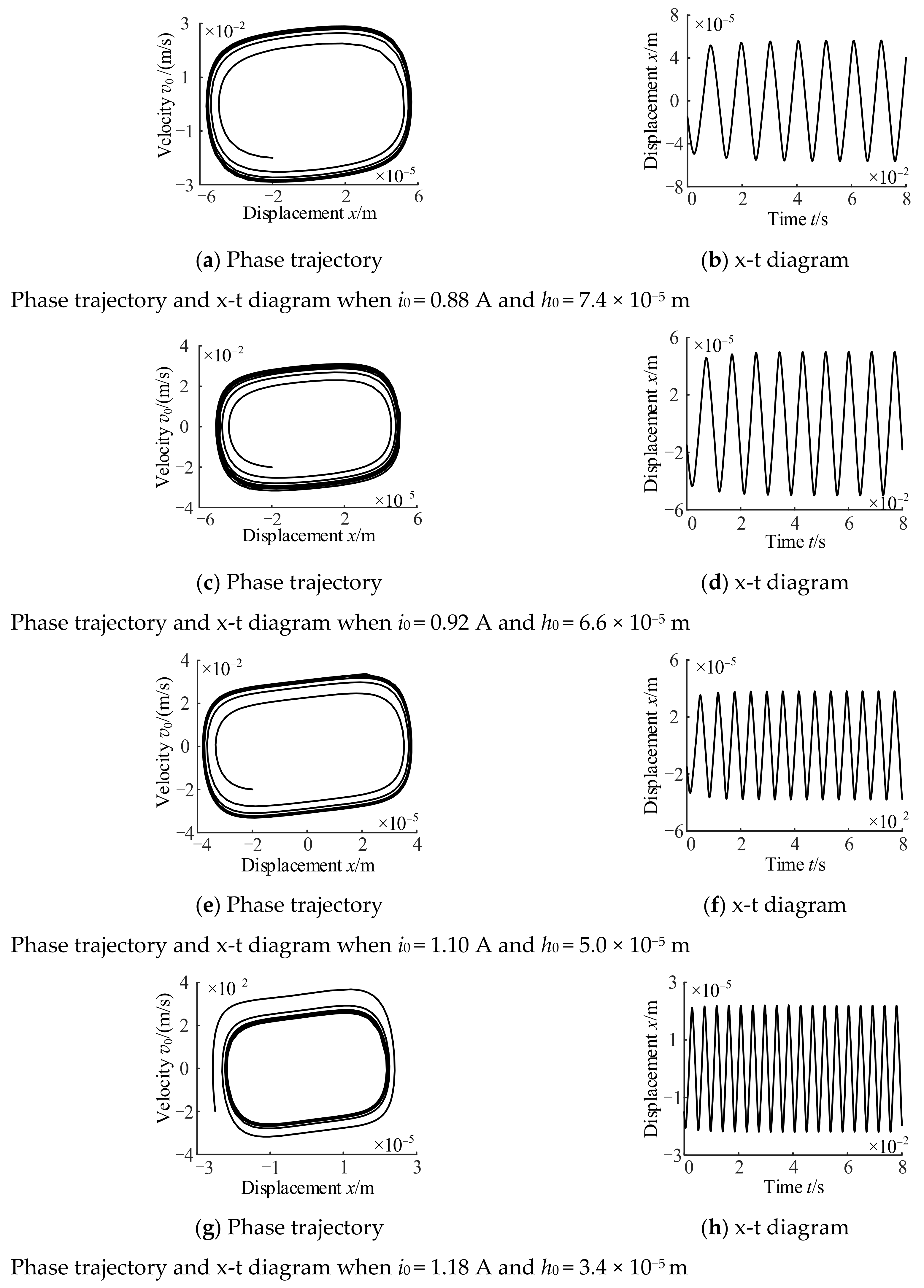
4.1.3. Phase Trajectory and X-T Diagram under The Combined Influence of Coil Current and Oil Film Thickness

The initial displacement x₀ and velocity v₀ were randomly selected, and the phase trajectory and x-t diagram were simulated as shown as Figure 10.

According to Figure 10, when i₀ increases from 0.88 A to 1.22 A and h₀ decreases from 7.4 × 10⁻⁵ m to 2.6 × 10⁻⁵ m, the vibration amplitude decrease from 5.6 × 10⁻⁵ m to 1.2 × 10⁻⁵ m. The maximum vibration velocity increases from 0.029 m/s to 0.033 m/s and then decreases to 0.018 m/s. Compared with i₀, the influence of h₀ on vibration amplitude is more obvious; accordingly, the maximum vibration velocity increases first and then decreases.

4.2. Experimental Result of Decoupling

4.2.1. Brief Introduction to MLDSB Testing System

The MLDSB testing system is composed of an electronic control system, a hydrostatic system, and a bearing body, as shown in Figure 11.

A hydrostatic system is a constant-pressure supporting model, and its flow is adjusted by needle valve. An electronic control system is a closed-loop position control system, and its current is adjusted by PD controller.

The parameters of the MLDSB testing system are as follows.

(1)

Hydraulic pump, model TGPVL4-200SH, pressure 14 MPa, flow 16 L/min, rotate speed 1450 r/min.

(2)

Relief valve, model DBD-H-6-P-10-B-NG10, pressure 10 MPa, size 6 mm.

(3)

Nozzle valve, model A7-2-KL2-0KL20-PTFE, size 6 mm.

(4)

Flow gauge, model LWGY-S, pressure 2 MPa, flow 120–2400 mL/min, and accuracy 2%.

(5)

Pressure gauge, model HSTL-802, pressure 10 MPa, accuracy 0.25%.

(6)

Displacement gauge, model VB-Z9900, range for 4 mm, accuracy 1.5%.

(7)

Coil, materials for Cu, diameter 1.0 mm, electrical resistivity 0.02240 Ω/m, length 25 m.

(8)

PC, model IPC-610L, mainboard AIMB-705BG, CPU I5-6500.

(9)

Output card, model NI6723, 8 channel output.

(10)

Input card, model PCI1716, 16 channel input,

(11)

12V Power, model S1500-12, voltage 12V, current 125 A, power 1500 W.

(12)

Power amplifier, model AQMD3620NS-A2, power 400 w, input voltage 36 V, current 16 A.

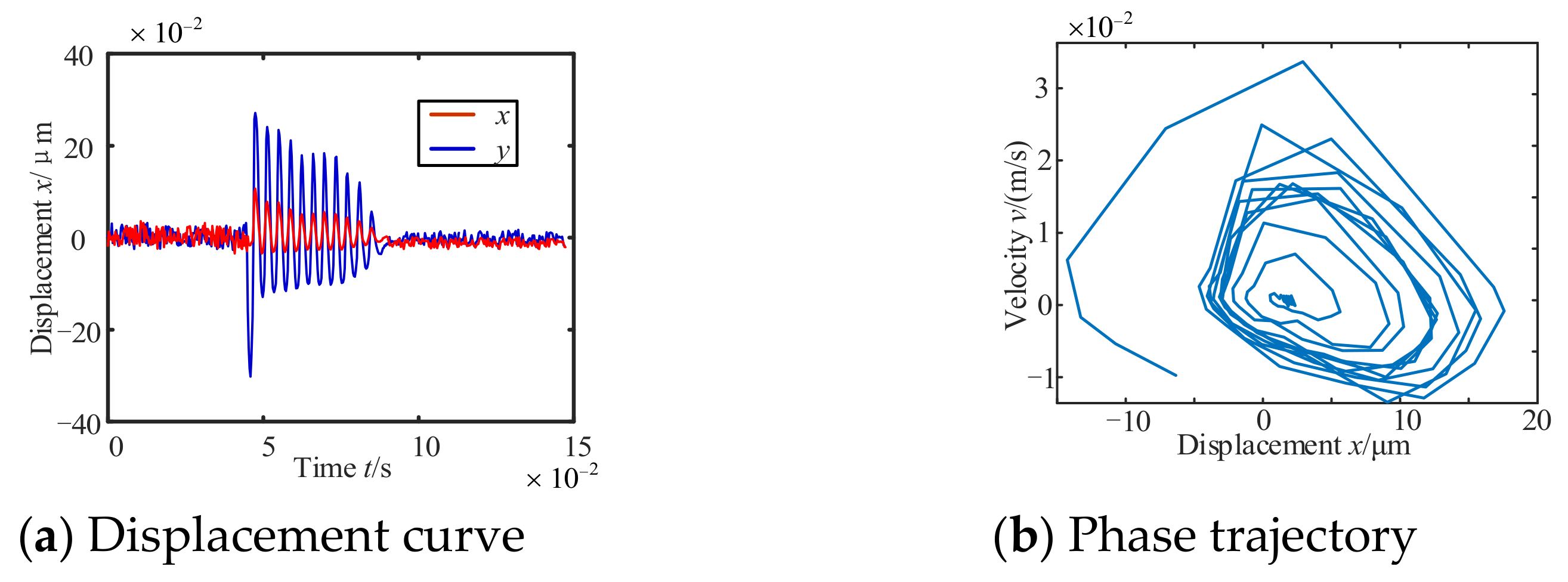
4.2.2. Analysis of Experimental Results

The displacement curves when i₀ = 0.5 A, 1.0 A, and 1.2 A are shown in Figure 12, Figure 13 and Figure 14.

It can be seen from the experimental results that the rotor can return to the original position and Hopf bifurcation does not occur at this time after the external interference disappears, when i₀ is 0.5 A. When i₀ is 1.0 A, the rotor gradually approaches equal amplitude oscillation and Hopf bifurcation occurs. When i₀ is 1.2 A, the rotor also gradually approaches equal amplitude oscillation. Compared with the case in which i₀ is 1.0 A, the oscillation amplitude increases, the adjustment time decreases, the maximum vibration speed increases, the oscillation phenomenon is more serious, and the stability of MLDSB becomes weaker.

5. Conclusions

(1)

The stable limit cycle and Hopf bifurcation occur when the coil current and oil film thickness are greater than the threshold; at this point, the bearing rotor features constant amplitude vibration and its motion loses stability. Therefore, in order to ensure the stable operation of the bearing rotor, the values of the coil current and oil film thickness should be set below the threshold, or the threshold should be avoided by adjusting other control parameters.

(2)

Under the combined influence of the coil current and oil film thickness, the boundary value of the Hopf bifurcation of the bearing system decreases, and the amplitude of the Hopf bifurcation’s out-of-limit cycle increases with the increase in the coil current and oil film thickness. In addition, compared with the coil current, the oil film thickness creates a greater impact on the vibration amplitude of the limit cycle. Therefore, in order to ensure the stable operation of the bearing rotor, we should try our best to ensure that the values of the coil current and oil film thickness are less than the boundary value of the Hopf bifurcation.

(3)

The Hopf bifurcation results obtained using the MLDSB Testing System show that Hopf bifurcation does not occur when i₀ < 0.5A, although it occurs when i₀ > 1.0A. Therefore, in order to ensure the stable operation of the bearing system, the coil current should be controlled below 1A as far as possible.

References

- Zhao, J.; Yan, W.; Wang, Z.; Gao, D.; Du, G. Study on Clearance-Rubbing Dynamic Behavior of 2-DOF Supporting System of Magnetic-Liquid Double Suspension Bearing. Processes 2020, 8, 973. [Google Scholar] [CrossRef]
- Zhao, J.; Wu, X.; Han, F.; Ma, X.; Yan, W.; Liang, Y.; Gao, D.; Du, G. Influence of Design Parameters on Static Bifurcation Behavior of Magnetic Liquid Double Suspension Bearing. Int. J. Aerosp. Eng. 2021, 2021, 6646235. [Google Scholar] [CrossRef]
- Zhang, B. Research on Decoupling Control of Magnetic-Fluid Double Suspension Bearing System. Master’s Thesis, Yanshan University, Qinhuangdao, China, 2018. [Google Scholar]
- Guo, W.; Yang, J.; Wang, M. Stability Analysis of Hydro-turbine Governing System of Hydropower Station with Inclined Ceiling Tailrace Based on Hopf Bifurcation. J. Hydraul. Eng. 2016, 47, 189–199. [Google Scholar]
- Wei, D.; Li, L.; Ke, X.; Ning, P.; Pan, Z. Lateral Stability and Hopf Bifurcation Characteristics of 4WS Vehicle Considering Body Roll. Trans. China Soc. Agric. Mach. 2015, 46, 343–363. [Google Scholar]
- Ding, J.; Ding, W.C.; De-Yang, L.I. Numerical Computation of Hopf Bifurcation and Limit Cycles for Nonlinear Conveyor Belt System. Mach. Des. Manuf. 2019, 2, 107–113. [Google Scholar]