
A Novel Emergency Gas-to-Power System Based on an Efficient and Long-Lasting Solid-State Hydride Storage System: Modeling and Experimental Validation

 ,
,  , ,
, ,  , ,
, , 


Abstract
:
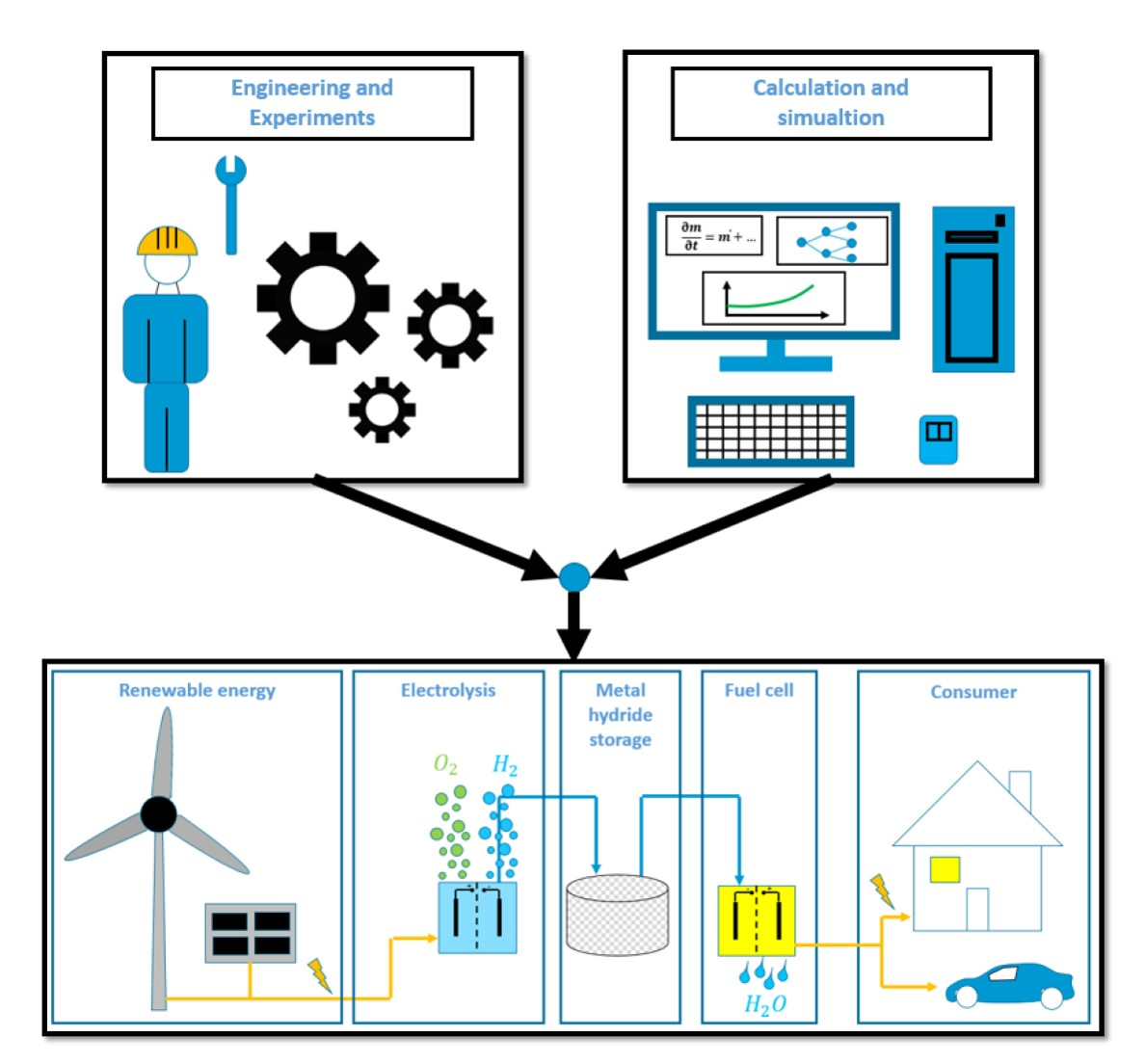
1. Introduction
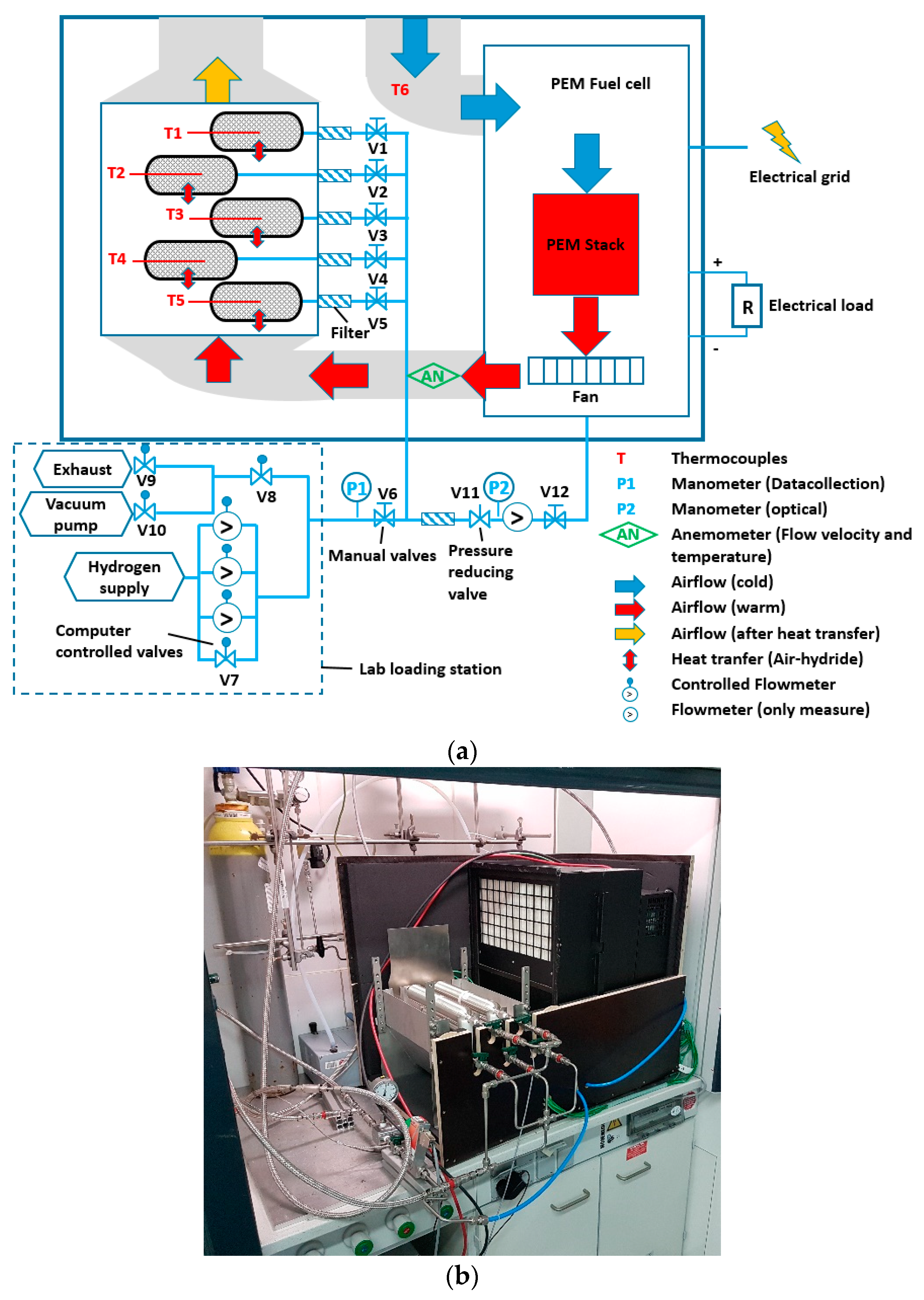
2. The Experimental Setup
2.1. Description of the Experimental Setup
2.2. Operating Scenarios and Test Parameters: MH2-Powerbank System
2.2.1. Operating Scenarios
2.2.2. Experimental Parameters
3. Mathematical Model
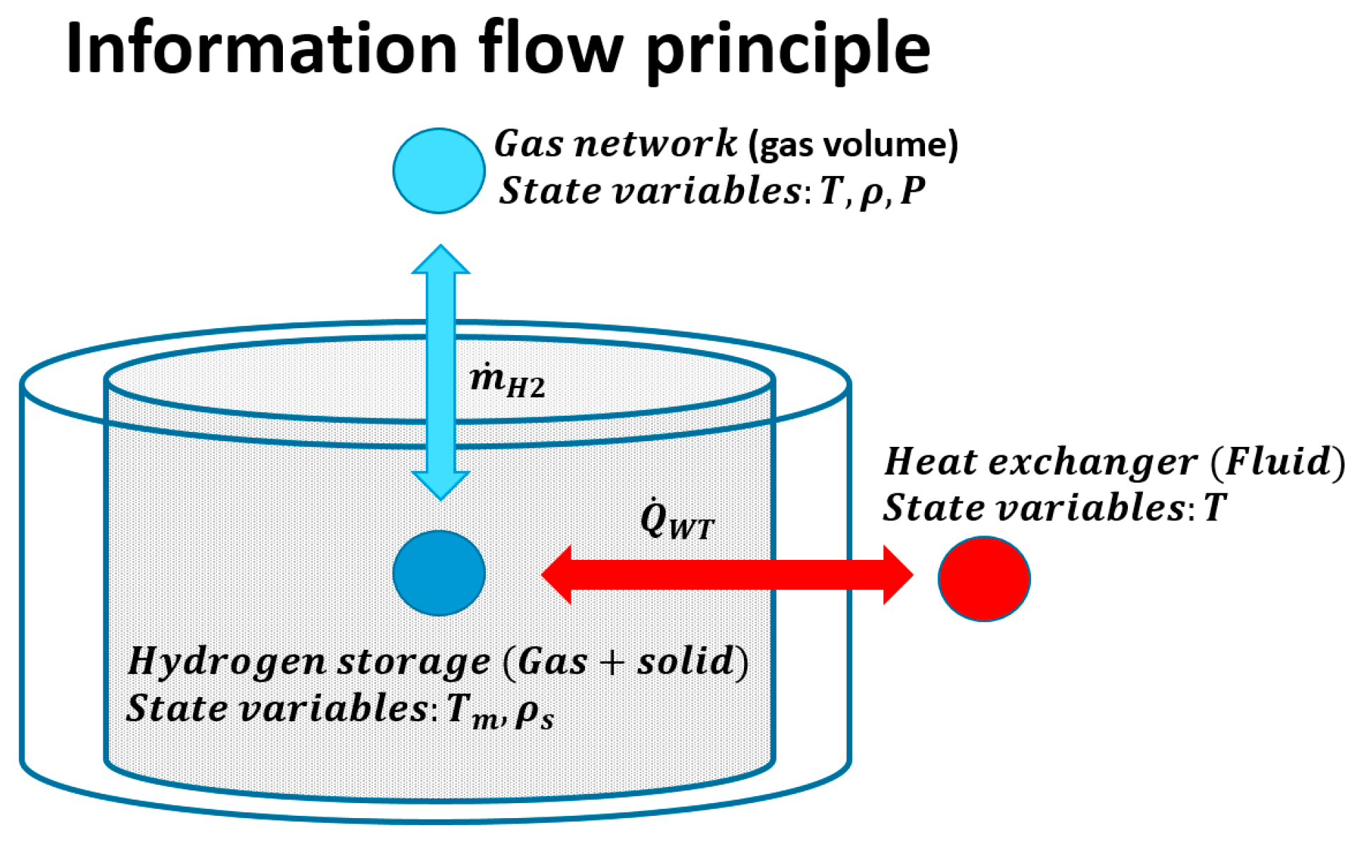
3.1. MH-Tanks and the Connections with the Network: Description of the 0D Model
- The hydrogen transport inside the porous medium’s free volume is neglected due to the fast hydrogen velocity.
- The local thermal equilibrium is assumed: temperatures in both fluid (hydrogen) and solid phases (alloy-hydride) are equal.
- Hydrogen is considered an ideal gas due to the low working pressures.
- The mass exchange caused by the chemical reaction occurs directly between the hydride-forming alloy and the connected gas network.
- The heat exchange between the gas network and the hydride material is neglected.
- The gas pressure in the porous bed (alloy-hydride) is assumed to be equal to that of the connected gas network. Therefore, the mass flow of hydrogen during the reaction occurs as part of the gas network.
- The temperature change of the gas phase due to gas transport between the gas phase and the solid hydride is neglected.
3.1.1. Thermodynamics of the Metal Hydride: Determination of the Equilibrium Pressure through Pressure-Composition-Isotherms (PCIs) Modeling
3.1.2. Kinetics of the Metal Hydride: Reaction Kinetic Model
3.1.3. Heat Exchange Modeling: Dehydrogenation of MH-Tanks by Utilizing the Fuel Cell Waste Heat
3.1.4. Model Implementations in Simscape
3.1.5. Boundary Conditions
3.1.6. Initial Condition and Simulation Parameters
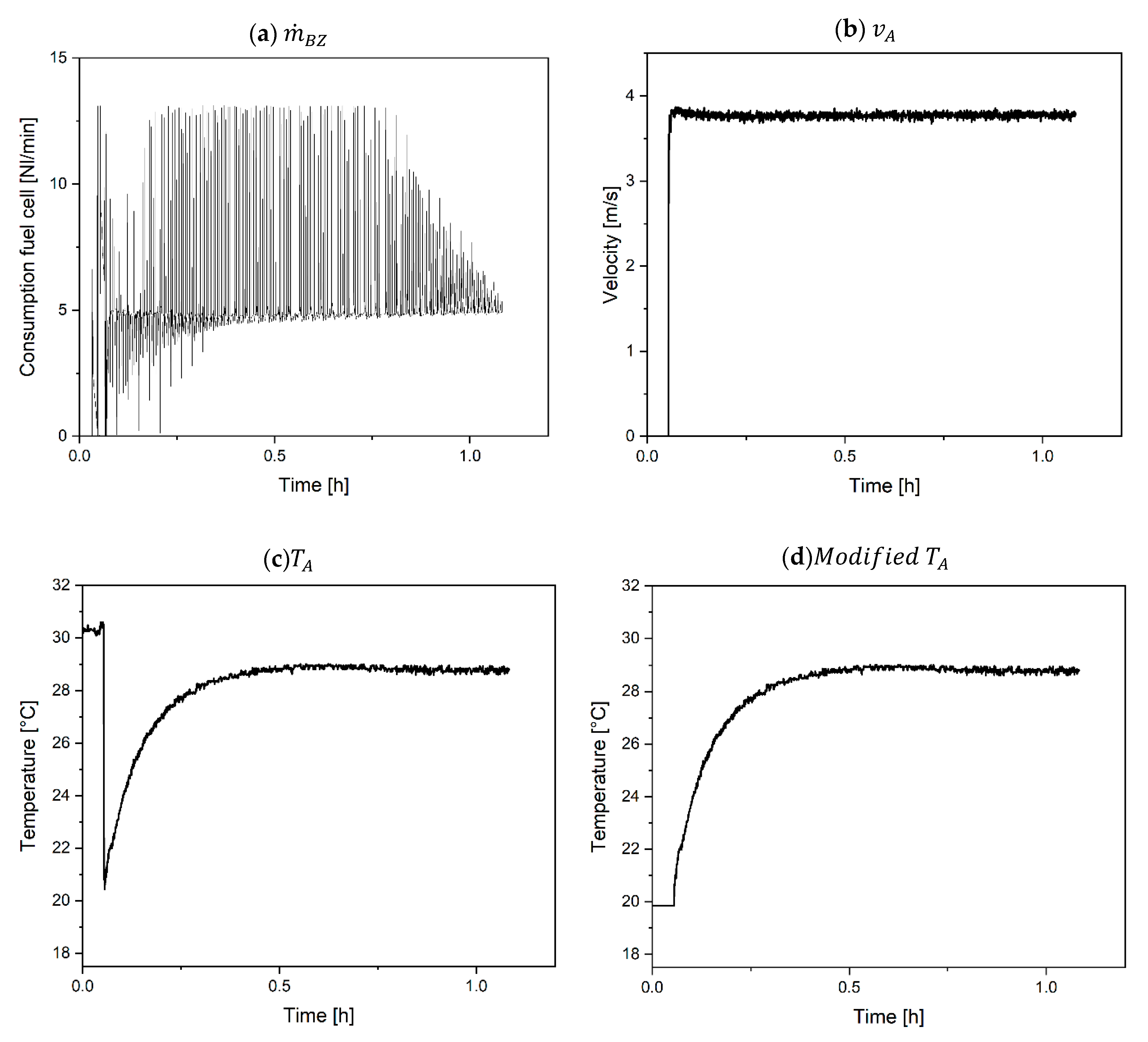
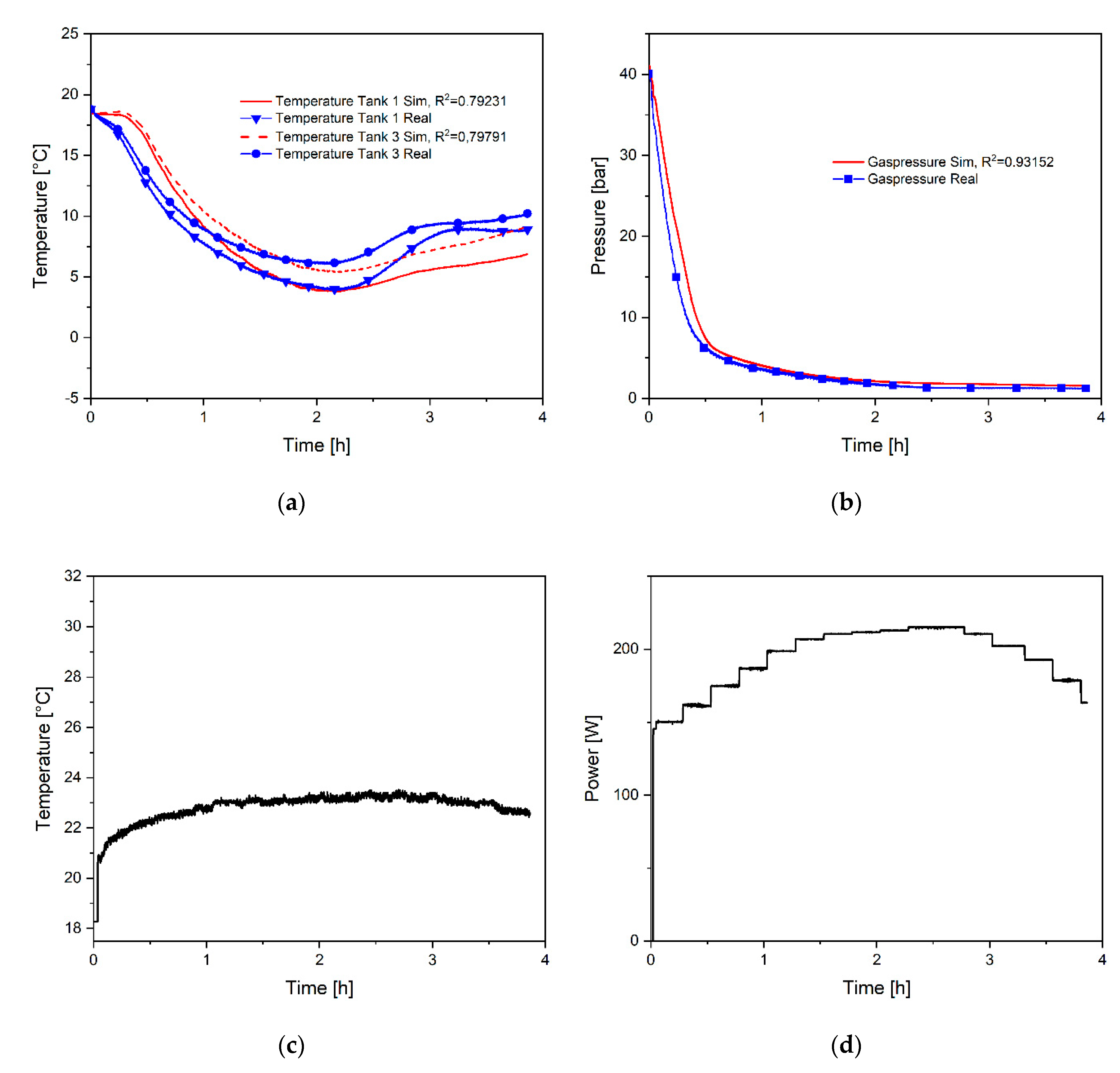
4. Model Validation and Discussion of the Results
5. Conclusions
Supplementary Materials
Author Contributions
Funding
Data Availability Statement
Acknowledgments
Conflicts of Interest
References
- Forest, G.; Markova, A. The Road to Carbon-Free Society; Climate Change Energy and Environment; Friedrich Ebert Stiftung: London, UK, 2021; Available online: http://library.fes.de/pdf-files/bueros/london/18473.pdf (accessed on 22 December 2021).
- Chitanava, M.; Janashia, N.; Samkhardze, I.; Vardosanidze, K. The Impact of Climate Change Mitigation Policy on Employment; Climate Basics; Friedrich Ebert Stiftung: Zagreb, Croatia, 2021; Available online: http://library.fes.de/pdf-files/bueros/georgien/17558.pdf (accessed on 22 December 2021).
- Munta, M. The European Green Deal; Climate Change Energiy and Environment; Friedrich Ebert Stiftung: Zagreb, Croatia, 2020; Available online: http://library.fes.de/pdf-files/bueros/kroatien/17217.pdf (accessed on 22 December 2021).
- Strunz, S.; Gawel, E.; Lehmann, P. The political economy of renewable energy policies in Germany and the EU. Util. Policy 2016, 42, 33–41. [Google Scholar] [CrossRef] [Green Version]
- Egeland-Eriksen, T.; Hajizadeh, A.; Sartori, S. Hydrogen-based systems for integration of renewable energy in power systems: Achievements and perspectives. Int. J. Hydrogen Energy 2021, 46, 31963–31983. [Google Scholar] [CrossRef]
- Gielen, D.; Boshell, F.; Saygin, D.; Bazilian, M.D.; Wagner, N.; Gorini, R. The role of renewable energy in the global energy transformation. Energy Strategy Rev. 2019, 24, 38–50. [Google Scholar] [CrossRef]
- Yue, M.; Lambert, H.; Pahon, E.; Roche, R.; Jemei, S.; Hissel, D. Hydrogen energy systems: A critical review of technologies, applications, trends and challenges. Renew. Sustain. Energy Rev. 2021, 146, 111180. [Google Scholar] [CrossRef]
- Muthukumar, P.; Groll, M. Metal hydride based heating and cooling systems: A review. Int. J. Hydrogen Energy 2010, 35, 3817–3831. [Google Scholar] [CrossRef]
- Rusman, N.A.A.; Dahari, M. A review on the current progress of metal hydrides material for solid-state hydrogen storage applications. Int. J. Hydrogen Energy 2016, 41, 12108–12126. [Google Scholar] [CrossRef]
- Bellosta von Colbe, J.; Ares, J.-R.; Barale, J.; Baricco, M.; Buckley, C.; Capurso, G.; Gallandat, N.; Grant, D.M.; Guzik, M.N.; Jacob, I.; et al. Application of hydrides in hydrogen storage and compression: Achievements, outlook and perspectives. Int. J. Energy Res. 2019, 44, 7780–7808. [Google Scholar] [CrossRef]
- Aldas, K.; Mat, M.D.; Kaplan, Y. A three-dimensional mathematical model for absorption in a metal hydride bed. Int. J. Hydrogen Energy 2002, 27, 1049–1056. [Google Scholar] [CrossRef]
- Lexcellent, C.; Gay, G.; Chapelle, D. Thermomechanics of a Metal Hydride Tank. Contiuum Mech. Thermodyn. 2014, 27, 379–397. [Google Scholar] [CrossRef]
- Muthukumar, P.; Ramana, S.V. Numerical simulation of coupled heat and mass transfer in metal hydride-based hydrogen storage reactor. J. Alloys Compd. 2009, 472, 466–472. [Google Scholar] [CrossRef]
- Kaplan, Y.; Veziroglu, T.N. Mathematical modelling of hydrogen storage in a LaNi5 hydride bed. Int. J. Energy Res. 2003, 27, 1027–1038. [Google Scholar] [CrossRef]
- Lahmer, K.; Bessaih, R. Impact of kinetic reaction models on hydrogen absorption in metal hydride tank modeling. Int. J. Hydrogen Energy 2015, 40, 13718–13724. [Google Scholar] [CrossRef]
- Mohammadshahi, S.; Gray, E.; Webb, C. A review of mathematical modelling of metal-hydride systems for hydrogen storage applications. Int. J. Hydrogen Energy 2016, 41, 3470–3484. [Google Scholar] [CrossRef]
- Lozano, G.A.; Na Ranong, C.; Von Colbe, J.M.B.; Bormann, R.; Fieg, G.; Hapke, J.; Dornheim, M. Empirical kinetic model of sodium alanate reacting system (II). Hydrogen desorption. Int. J. Hydrogen Energy 2010, 35, 7539–7546. [Google Scholar] [CrossRef] [Green Version]
- Lozano, G.A.; Na Ranong, C.; von Colbe, J.M.B.; Bormann, R.; Hapke, J.; Fieg, G.; Klassen, T.; Dornheim, M. Optimization of hydrogen storage tubular tanks based on light weight hydrides. Int. J. Hydrogen Energy 2012, 37, 2825–2834. [Google Scholar] [CrossRef]
- Jana, S.; Muthukumar, P. Design and Performance Prediction of a Compact MmNi4.6Al0.4 based Hydrogen Storage System. J. Energy Storage 2021, 39, 102612. [Google Scholar]
- Stark, M.; Krost, G. Neural network based modeling of metal-hydride bed storages for small selfsustaining energy supply systems. In Proceedings of the 2011 IEEE Trondheim PowerTech, Trondheim, Norway, 19–23 June 2011. [Google Scholar]
- Bedrunka, M.; Bornemann, N.; Steinebach, G.; Reith, D. Reaction behavior modeling of metal hydride based on FeTiMn using numerical simulations. 2021. submitted. [Google Scholar]
- Nasrallah, S.; Jemni, A. Heat and mass transfer models in metal-hydrogen reactor. Int. J. Hydrogen Energy 1997, 22, 67–76. [Google Scholar] [CrossRef]
- Steinebach, G.; Dreistadt, D.M. Water and Hydrogen Flow in Networks: Modelling and Numerical Solution by ROW Methods. In Rosenbrock—Wanner–Type Methods; Springer: Cham, Switzerland, 2021; pp. 19–47. [Google Scholar]
- Steinebach, G.; Dreistadt, D.; Hausmann, P.; Jax, T. Setup of Simulation Model and Calibration. In Decision Support Systems for Water Supply Systems; European Mathematical Society Publishing House: Berlin, Germany, 2020; pp. 129–149. [Google Scholar]
- Dematteis, E.M.; Dreistadt, D.M.; Capurso, G.; Jepsen, J.; Cuevas, F.; Latroche, M. Fundamental hydrogen storage properties of TiFe-alloy with partial substitution of Fe by Ti and Mn. J. Alloys Compd. 2021, 874, 159925. [Google Scholar] [CrossRef]
- HyCare. Hydrogen CArrier for Renewable Energy Storage. Available online: https://hycare-project.eu/ (accessed on 22 December 2021).
- Fünfgeld, C. Repräsentatives Profil “Haushalt”. 1999. Available online: https://www.bdew.de/energie/standardlastprofile-strom/ (accessed on 22 December 2021).
- The MathWorks Inc. Simscape Modellieren und Simulieren von Physikalischen Mehrdomänen Systemen. Available online: https://de.mathworks.com/products/simscape.html (accessed on 22 December 2021).
- The MathWorks Inc. Constant Volume Chamber (G). Available online: https://de.mathworks.com/help/physmod/simscape/ref/constantvolumechamberg.html (accessed on 22 December 2021).
- Feng, F.; Geng, M.; Northwood, D. Mathematical model for the plateau region of P–C-isotherms of hydrogen-absorbing alloys using hydrogen reaction kinetics. Comput. Mater. Sci. 2002, 23, 291–299. [Google Scholar] [CrossRef]
- Schwarz, R.B.; Khachaturyan, A.G. Thermodynamics of open two-phase systems with coherent interfaces. Phys. Rev. Lett. 1995, 74, 2523–2526. [Google Scholar] [CrossRef] [PubMed]
- Schwarz, R.; Khachaturyan, A. Thermodynamics of open two-phase systems with coherent interfaces: Application to metal–hydrogen systems. Acta Mater. 2006, 54, 313–323. [Google Scholar] [CrossRef]
- Buchner, H. Energiespeicherung in Metallhydriden; Springer: New York, NY, USA, 1982. [Google Scholar]
- Herbrig, K.; Röntzsch, L.; Pohlmann, C.; Weißgärber, T.; Kieback, B. Hydrogen storage systems based on hydride–graphite composites: Computer simulation and experimental validation. Int. J. Hydrogen Energy 2013, 38, 7026–7036. [Google Scholar] [CrossRef]
- Liebig, C.D.D. Systemsimulation und Versuchsdurchführung eines auf PEM Brennstoffzellen Basierten Gas-to-Power-Systems mit Integrierten Metallhydridspeichern. Master’s Thesis, Helmut-Schmidt-Universität Universität der Bundeswehr Hamburg, Hamburg, Germany, 2021. [Google Scholar]
- Gnielinski, V. G6 Querumströmte Einzelne Rohre, Drähte und Profilzylinder. In VDI-Wärmeatlas; Verein Deutscher Ingenieure: Düsseldorf, Germany, 2013; pp. 817–822. [Google Scholar]
- The MathWorks Inc. Pipe (G). Available online: https://de.mathworks.com/help/physmod/simscape/ref/pipeg.html (accessed on 22 December 2021).
- Covarrubias Guarneros, M. Modeling and Parameterization of a PEM Fuel Cell Stack for System Integration into a Metal Hydride Based Hydrogen Storage System. Master’s Thesis, Hamburg University of Applied Sciences, Hamburg, Germany, 2021. [Google Scholar]
- Kümmel, W. Technische Strömungsmechanik: Theorie und Praxis; Vieweg+Teubner Verlag: Wiesbaden, Germany, 2004. [Google Scholar]
- Gambini, M.; Manno, M.; Vellini, M. Numerical analysis and performance assessment of metal hydride-based hydrogen storage systems. Int. J. Hydrogen Energy 2008, 33, 6178–6187. [Google Scholar] [CrossRef]
- Muthukumar, P.; Maiya, M.P.; Murthy, S.S. Experiments on a metal hydride-based hydrogen storage device. Int. J. Hydrogen Energy 2005, 30, 1569–1581. [Google Scholar] [CrossRef]
- Capurso, G.; Schiavo, B.; Jepsen, J.; Lozano, G.A.; Metz, O.; Klassen, T.; Dornheim, M. Metal Hydride-Based Hydrogen Storage Tank Coupled with an Urban Concept Fuel Cell Vehicle: Off Board Tests. Adv. Sustain. Syst. 2018, 2, 1800004. [Google Scholar] [CrossRef]


| Experiment | Resistance [Ohm] | Duration [h] | Power [W] |
|---|---|---|---|
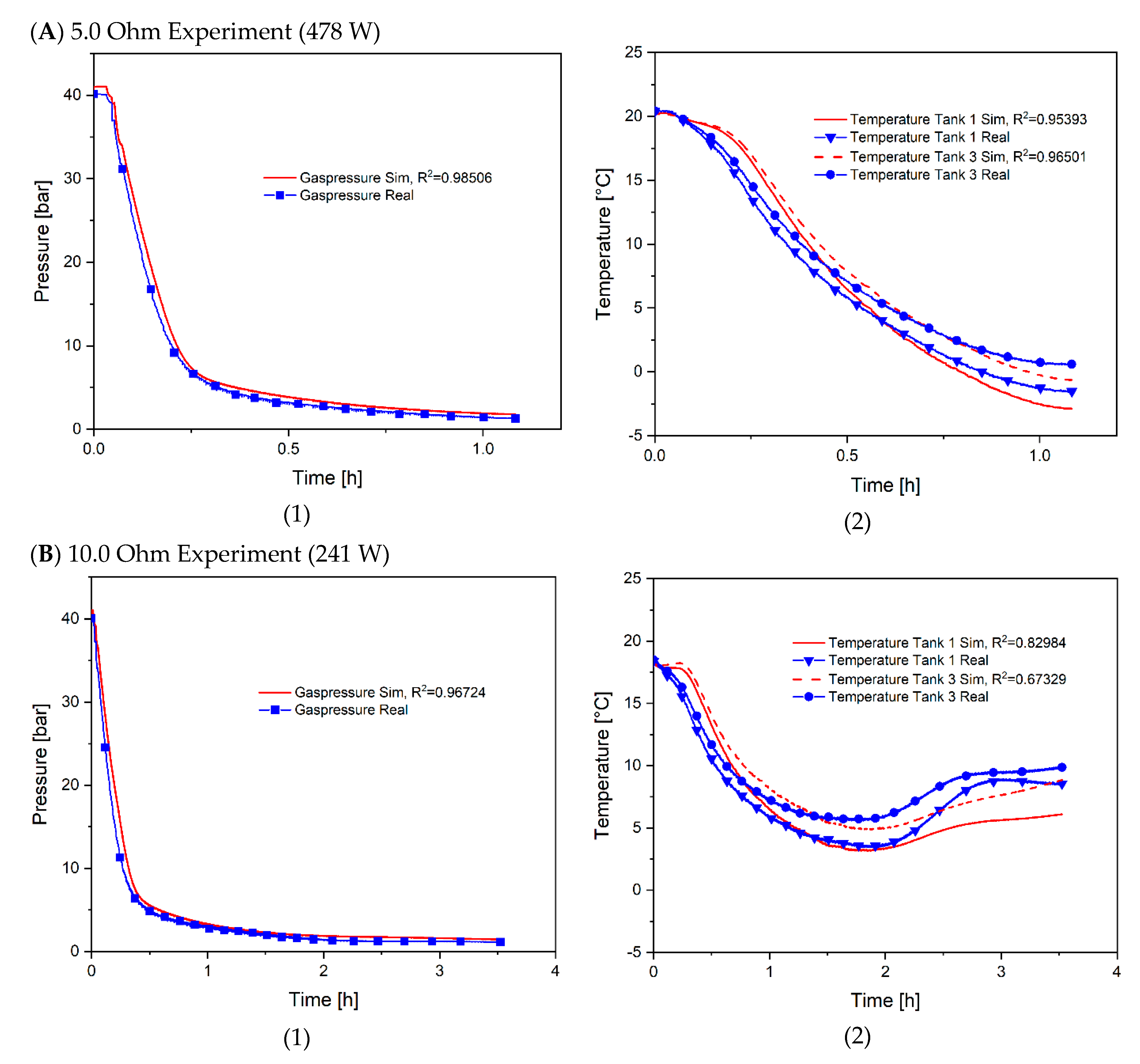
| 1 | 5.0 | 1.13 | 478 |
| 2 | 7.5 | 1.91 | 319 |
| 3 | 10.0 | 3.55 | 241 |
| 4 | 20.0 | 6.5 | 120 |
| 5 | Large variations of power consumption | 2.01 | 149–596 |
| 6 | Representative of the daily profile | 3.88 | 152–213 |
| Coefficients | Absorption | Desorption | Coefficients | Absorption | Desorption |
|---|---|---|---|---|---|
| Parameter | Value | Unit | Description |
|---|---|---|---|
| From 17 to 21 | °C | Range of initial measured temperature for the tanks | |
| 3250.04 | Initial crystalline density full load (considering the experimental gravimetric capacity: 1.54 wt.%) | ||
| 40 | bar | Initial gas pressure under hydrogenated state. |
| Parameter | Value | Unit | Description | Parameter | Value | Unit | Description |
|---|---|---|---|---|---|---|---|
| 2.6536 | Reaction kinetic constant of abs. | From −33,638 to−28,211 | Enthalpy of abs. in the range of 0.2–1.3 wt.% | ||||
| 0.8852 | Reaction kinetic constant of des. | From −34,917 to −29,969 | Enthalpy of des. in the range of 0.2–1.3 wt.% | ||||
| 17,500 | Activation energy of abs. | 3200 | Minimal bulk density | ||||
| 13,750 | Activation energy of des. | 3250.04 | Maximal bulk density | ||||
| 682.4 | Heat capacity | 0.5 | Porosity | ||||
| 5–6.2 | Thermal conductivity solid | 0.163–0.227 | Thermal conductivity gas [39] |
Publisher’s Note: MDPI stays neutral with regard to jurisdictional claims in published maps and institutional affiliations. |
© 2022 by the authors. Licensee MDPI, Basel, Switzerland. This article is an open access article distributed under the terms and conditions of the Creative Commons Attribution (CC BY) license (https://creativecommons.org/licenses/by/4.0/).
Share and Cite
Dreistadt, D.M.; Puszkiel, J.; Bellosta von Colbe, J.M.; Capurso, G.; Steinebach, G.; Meilinger, S.; Le, T.-T.; Covarrubias Guarneros, M.; Klassen, T.; Jepsen, J. A Novel Emergency Gas-to-Power System Based on an Efficient and Long-Lasting Solid-State Hydride Storage System: Modeling and Experimental Validation. Energies 2022, 15, 844. https://doi.org/10.3390/en15030844
Dreistadt DM, Puszkiel J, Bellosta von Colbe JM, Capurso G, Steinebach G, Meilinger S, Le T-T, Covarrubias Guarneros M, Klassen T, Jepsen J. A Novel Emergency Gas-to-Power System Based on an Efficient and Long-Lasting Solid-State Hydride Storage System: Modeling and Experimental Validation. Energies. 2022; 15(3):844. https://doi.org/10.3390/en15030844
Chicago/Turabian StyleDreistadt, David Michael, Julián Puszkiel, José Maria Bellosta von Colbe, Giovanni Capurso, Gerd Steinebach, Stefanie Meilinger, Thi-Thu Le, Myriam Covarrubias Guarneros, Thomas Klassen, and Julian Jepsen. 2022. "A Novel Emergency Gas-to-Power System Based on an Efficient and Long-Lasting Solid-State Hydride Storage System: Modeling and Experimental Validation" Energies 15, no. 3: 844. https://doi.org/10.3390/en15030844
APA StyleDreistadt, D. M., Puszkiel, J., Bellosta von Colbe, J. M., Capurso, G., Steinebach, G., Meilinger, S., Le, T.-T., Covarrubias Guarneros, M., Klassen, T., & Jepsen, J. (2022). A Novel Emergency Gas-to-Power System Based on an Efficient and Long-Lasting Solid-State Hydride Storage System: Modeling and Experimental Validation. Energies, 15(3), 844. https://doi.org/10.3390/en15030844