Numerical Simulations of Air Flow and Traffic–Related Air Pollution Distribution in a Real Urban Area

Abstract

With increasing urbanization, urban air pollutants are becoming more and more relevant to human health. Here, combined with meteorological observation data, a numerical simulation of typical urban blocks in Shanghai was carried out to understand the spread of air pollutants caused by road traffic sources (ground–level and viaduct–level). Firstly, we analyzed the wind environment characteristics. Then, we quantitatively analyzed the pollutant distribution profiles and the contributions of two pollutant sources (PSV). Finally, we analyzed seven urban morphological parameters based on ventilation efficiency indices. Results revealed the following. (1) Ventilation patterns within the architectural complex are determined by local geometry; (2) Pollutants released at ground level were dominant when the Z–plane < 8 m high, and pollutants released from the viaduct source were 0.8–6.1% higher when the Z–plane ≥ 8 m high; (3) From ground level to a height of 60 m, the spatially–averaged normalized concentration (C*) tended to decrease gradually with distance from the source. C* increased irregularly with an increase in distance between 60 m and 86 m. Above 86 m, C* tended to increase linearly; (4) Vertical profiles of C* around buildings were building–specific, and their rate of change was inconsistent with height increases. In general, the correlations between C* and VR_w, and between C* and KE_turb were larger on the windward side of PSV upstream buildings than on the leeward side. Buildings downstream of the PSV showed the opposite situation; (5) At pedestrian level, the seven urban morphological parameters had no significant correlation with VR_w, C_ir*, and C_zs*.

1. Introduction

In 2018, around 55% of the world’s population lived in urban areas [1]. By 2030, this percentage will rise to 60%, and an estimated one–third of the global population will be living in cities with at least half a million inhabitants [2]. More and more high–rise buildings are being constructed worldwide. Taking Shanghai, a representative city in China, as an example, the number of buildings above eight stories increased from 121 in 1980 to 49,352 in 2019 [3]. Urbanization has thus caused continuing increases in the pervasiveness of street canyons in cities. In addition, air quality is deteriorating in many countries around the world that are undergoing rapid urbanization [4,5]. Urban air pollutants (such as nitrogen oxides, fine particulate matter (PM_2.5), and so on) greatly deteriorate air quality and have become a serious threat to public health [6,7]. Road traffic is considered a major source of PM_2.5 and NO₂ [8,9]. Xin et al. [10] found that during the COVID-19 lockdown in 2020, road traffic in Beijing decreased by 46.9%, while PM_2.5 and NO₂ concentrations decreased by 5.6% and 29.2%, respectively, compared with the same period in 2019. Therefore, it is important to study the distribution of traffic–related air pollutants in urban street canyons and the correlation between the morphological characteristics of different residential areas. This has been investigated through field measurements, wind tunnel experiments, and CFD simulations.

For the field measurement approach, spatial statistics were used to figure out the influence of the built–up environment on PM_2.5 concentrations. Yuan et al. [11] studied the urban morphological characteristics affecting the PM_2.5 concentration in Wuhan and found that building density (BD) and floor area ratio (FAR) were the most significant parameters. In past decades, traditional field measurements were frequently utilized in urban air pollutant studies. Based on data obtained from air quality monitoring stations (AQMS), a lot of research has focused on time–series analyses on horizontal scales near urban and regional surfaces [12,13,14]. Edussuriya et al. [15] investigated urban form variables for different city blocks by using field monitoring data. However, the spatial representativeness of urban AQMS was small [16]. Hence, other methodologies were based on unmanned aerial vehicles or the use of buildings and towers as observation platforms [17,18,19], which can further uncover the exchange mechanism in the atmosphere. Fan et al. [20] studied the physical formation mechanism of high concentrations of PM_2.5 pollution episodes by using a 325 m tower in Beijing. With the help of unmanned aerial vehicles, Peng et al. [21] found that PM_2.5 concentrations decreased as height increased, except when an air temperature inversion layer appeared. In addition to field measurements, wind tunnel and water channel experiments were employed to investigate pollutant dispersion [22,23,24]. Murakami et al. [25] analyzed the mechanism of wind acceleration at ground level by wind tunnel experiments. In their study, they found that changes to the basic shape of a building typically tended to produce an extensive deterioration of local wind conditions compared to the reference building. Tominaga et al. [26] investigated the impact of high–rise buildings on the pedestrian wind environment using wind tunnel tests. They found that a high–rise building significantly enlarged the static pressure difference between the windward and leeward walls below the street canyon level. However, in the above studies, measurements focused only on idealized neighborhoods. Moreover, the pollutant diffusion mechanism is being studied more and more by using computational fluid dynamics (CFD).

CFD technology has been successfully applied to the study of the wind environment and air pollutant dispersion in urban areas. Tominaga et al. [26] studied practical applications of CFD to pedestrian wind environments around buildings. A large number of CFD simulations have been carried out to study the characteristics of pedestrian–level wind around buildings [27,28,29]. In addition, a number of studies have investigated pollutant transport in a two–dimensional (2D) street canyon [30,31,32,33,34]. Hang et al. [35] investigated the effects of a viaduct on pollutant dispersion in 2D street canyons. They found that a viaduct significantly reduces overall spatial mean indoor concentrations of gaseous pollutants. Researchers have used CFD to simulate pollutant spread in three–dimensional (3D) idealized urban block models [36,37,38,39,40,41]. Hu et al. [38] used CFD to simulate an idealized urban block model of pollutant diffusion and found that low building density (BD) resulted in higher ventilation efficiency. Jiang et al. [42] investigated two residential neighborhoods with different BD and FAR by CFD and found that five key urban form parameters (BD, average building height (AH), building height standard deviation (SDH), average building volume (MBV), and enclosure degree (DE)) significantly affected the diffusion and distribution of pollutants in the neighborhood. Silva et al. [36] evaluated pollutant dispersion phenomena and found that the local ventilation performance strongly depends on block typology. Hang et al. [43] investigated the effect of building height variability on pollutant dispersion and pedestrian ventilation in idealized high–rise urban areas. Their results showed that larger height variations produce better pedestrian ventilation and lowering aspect ratios or increasing street lengths may strengthen the contribution of turbulent diffusions in removing pollutants for arrays with uniform building heights. Zhang et al. [44] numerically simulated the impact of a viaduct on flow within urban street canyons. They concluded that viaducts might reduce pollution levels in a street canyon. In addition, the impacts of viaduct settings and street aspect ratios on personal intake fraction in urban–like geometries were also studied [45]. Various influential factors on pollutant dispersion, such as different L/H (ratio of building length L to building height H) [46], canyon geometry [47], roof shapes of upwind and downwind buildings [48], and a number of vortices [49] were examined by CFD technology. Numerical results revealed that the distribution of pollutants in street canyons can be largely explained in terms of vortex circulation, and ventilation rate can be greatly improved when small building coverage ratios and large passage widths are maintained. Thus, it is important to optimize the layout design of community buildings to reduce pollutant levels.

As discussed above, for field measurements, the sparsity of observation stations makes it difficult to study high–resolution air pollutant concentration distributions. For numerical simulation, most studies have focused on pedestrian–level wind environments considering ground–level pollution or viaduct–level pollution using idealized urban block models and inlet profiles. In actual urban blocks, more and more high–rise buildings and complex traffic road networks make it necessary to consider both ground–level and elevated road pollution sources. In addition to pedestrian height in study areas, it is also necessary to consider the area surrounding the building because people spend most of their time indoors working and living. Air pollutant concentrations around buildings are closely related to indoor control quality.

Therefore, in this study, a real block model and statistical data from nearby weather stations were utilized to perform numerical simulation calculations. Both ground and elevated pollution sources were considered. Pollutant diffusion with distance at different heights was studied. The characteristics of vertical and horizontal concentration distribution were also studied, and the reason for the abnormal vertical distribution of concentration is explained. A total of 29 urban morphological parameters of ventilation efficiency indices were analyzed.

2. Outline of Numerical Simulations

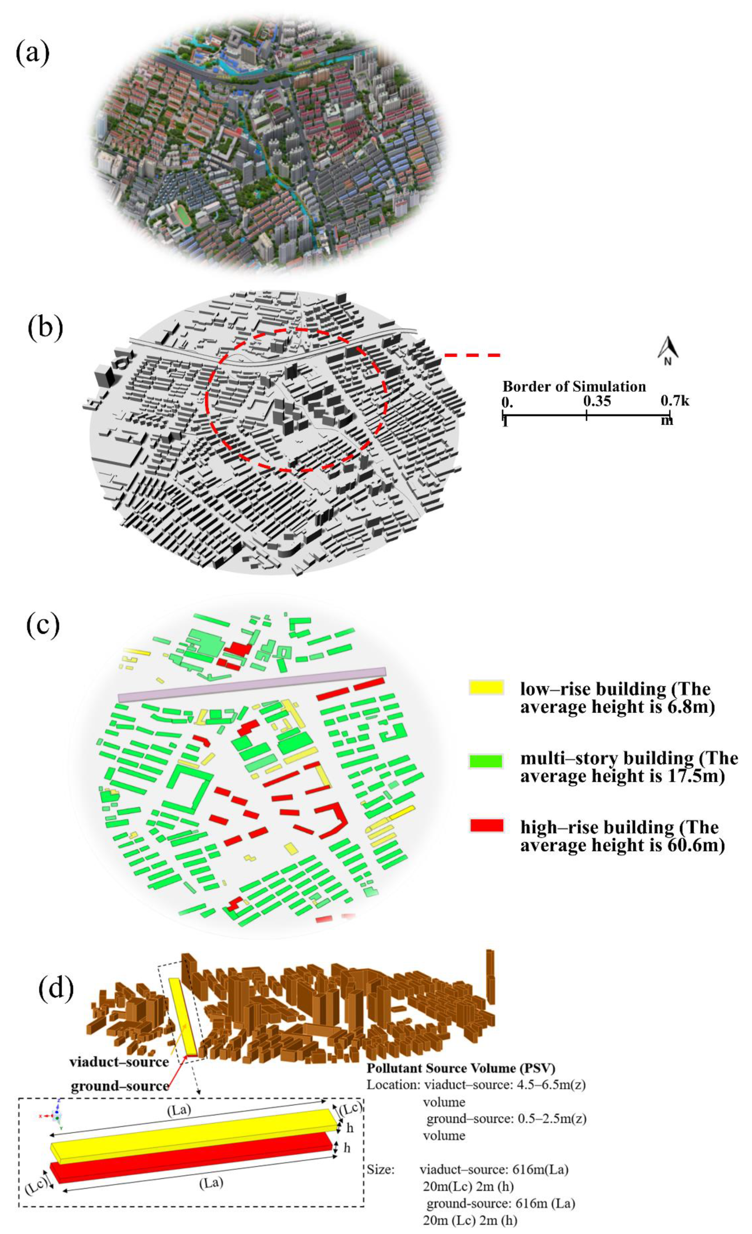
2.1. Urban Model

We take typical residential areas (Figure 1a) in Shanghai, China as the research area, which covers an area of approximately 4900 square meters. This area was chosen because similar urban arrangements can be seen in many regions of rapidly urbanizing China. Figure 1a,b shows a schematic diagram of the study area. In the CFD simulation, a 1:1 full–scale model of the urban area is established. The main research domains have dimensions of 700 m × 700 m in the east–west (x) and north–south (y) directions (red circle in Figure 1b). The computational domain contained 237 buildings and 2 roads (ground–level and viaduct–level). The 237 buildings were divided into 3 types: low–rise (average height 6.8 m), multi–story (average height 17.5 m), and high–rise buildings (average height 60.6 m) (Figure 1c) according to “Concrete Structure Technical Regulations for High–rise Buildings.”

2.2. Numerical Model

ANSYS Fluent 2020 was employed for the simulation. The finite volume method was used to discretize the control equation, and the SIMPLE algorithm was adopted for the velocity–pressure calculation. The Schmidt number was set to 0.9. The standard $k$–$\epsilon$ turbulence model was shown to accurately replicate the field measurements [50,51,52,53]. Thus, it was used to calculate the airflow. This model can also significantly save computational resources [51]. The QUICK scheme was applied to the convection terms of momentum, turbulent kinetic energy, and turbulent dissipation rate (Supplementary Materials Table S1).

The mass, momentum conservation Equations (1)–(4) and the transport equations for turbulent kinetic energy $k$ and turbulence dissipation rate $\epsilon$ Equations (5) and (6) are as follows:

$$\frac{\partial U_i}{\partial x_i}=0$$

(1)

$$U_j\frac{\partial U_j}{\partial x_j}=-\frac{1}{\rho }\frac{\partial P}{\partial x_i}+\frac{\partial }{\partial x_j}(v\frac{\partial U_i}{\partial x_j}-\overline{u_i{u}_j})$$

(2)

where:

$$\overline{u_i{u}_j}=\frac{2}{3}k{\delta }_i{}_j-v_t(\frac{\partial U_i}{\partial x_j}+\frac{\partial U_j}{\partial x_j})$$

(3)

and

$$v_t{=\mathrm{C}}_{\mu }\frac{k^2}{\epsilon }$$

(4)

$$U_j\frac{\partial k}{\partial x_j}=\frac{\partial }{\partial x_j}(\frac{v_t}{{\sigma }_k}·\frac{\partial k}{\partial x_j})+v_t(\frac{\partial U_i}{\partial x_j}+\frac{\partial U_j}{\partial x_i})\frac{\partial U_i}{\partial x_j}-\epsilon$$

(5)

$$U_j\frac{\partial \epsilon }{\partial x_j}=\frac{\partial }{\partial x_j}(\frac{v_t}{{\sigma }_{\epsilon }}·\frac{\partial \epsilon }{\partial x_j})+C_{\epsilon }{}_1\frac{\epsilon }{k}{v}_t((\frac{\partial U_i}{\partial x_j}+\frac{\partial U_j}{\partial x_i})\frac{\partial U_i}{\partial x_j})-C_{\epsilon }{}_2\frac{{\epsilon }^2}{k}$$

(6)

where $P$ is the mean pressure, $\overline{u_i{u}_j}$ is the Reynolds stress tensor, $k$ is the turbulent kinetic energy, $\epsilon$ denotes the turbulent dissipation rate, ${\delta }_i{}_j$ is the Kronecker delta, $v_t$ is the turbulent viscosity. The five empirical modelling constants are used as follows: ${\sigma }_k$ = 1.0, ${\sigma }_{\epsilon }$ = 1.3, $C_{\epsilon }{}_1$ = 1.44, $C_{\epsilon }{}_2$ = 1.92, $C_{\mu }$ = 0.09 [53].

In this study, two passive scalar transport equations were solved simultaneously to simulate the pollutant dispersion from ground–level and viaduct as follows (7):

$$\frac{\partial \rho {\phi }_k}{\partial t}+\frac{\partial }{\partial x_i}(\rho U_i{\phi }_k-\Gamma { }_k\frac{\partial {\phi }_k}{\partial x_i})=S{\phi }_k$$

(7)

where ${\Gamma }_k$ and $S{\phi }_k$ are the diffusion coefficient and source term for each of the scalar equations.

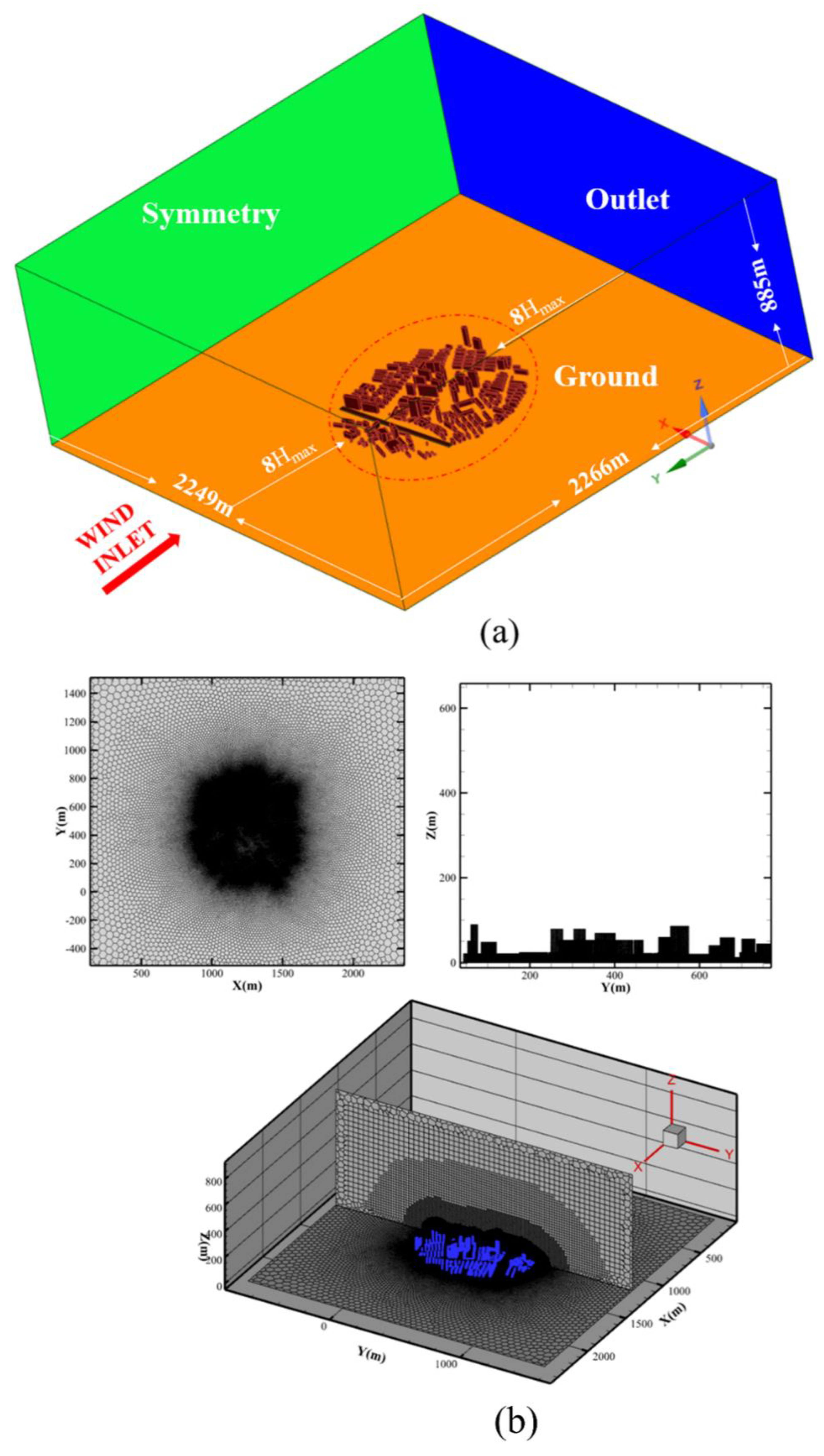
2.3. Meshing and Boundary Conditions

Figure 2b shows the total of 6,734,290 meshing grid cells. An unstructured polyhedral mesh was adopted in the computational domain because of its flexibility with the complex building geometry and because it alleviated computational load [54]. The meshes were refined on the building surface, and five prism layer meshes were used on the ground near the wall (the prism layer cell sizes adjacent to the building surface were 0.4 m, and the cell growth rate was uniform). Overall mesh quality was 0.732.

A 3D city model (Figure 2a) was designed using the Rhino and Arcmap software. The boundary conditions were set according to AIJ guidelines [26,55] (Figure 2a). The overall dimensions of the domain in the x, y, and z directions were 2249 m, 2266 m, and 885 m, respectively.

Considering the different prevailing wind directions in each season, the pollutant distributions have seasonal characteristics [56]. A power law was employed for the inlet velocity profile u (

Table 1. Calculation conditions.

Code	Fluent 2020 R2
Tubulence	Standard $k$–$\epsilon$ model
Inlet	u = Uref (z/zref) α, α = 0.27, zref = 79 m, Uref = 4.64 m/s $k$ = (I(z)u(z))2, I(z) = 0.1(z/zG)−α−0.05, zG = 550 m $\mathsf{\epsilon }=\mathrm{C}{}_u^{1/2}$$k$$\left(\mathrm{z}\right)\frac{d(u(z))}{dz}$, Cu = 0.09
Outlet	Outflow
Upper and side surface	Symmetry
Building surface and ground	Wall function
Overall Summary (grid)	6,734,290

). The U_ref, z_ref, and wind directions were chosen based on the data from field weather stations monitoring in winter, as shown in Figure 3.

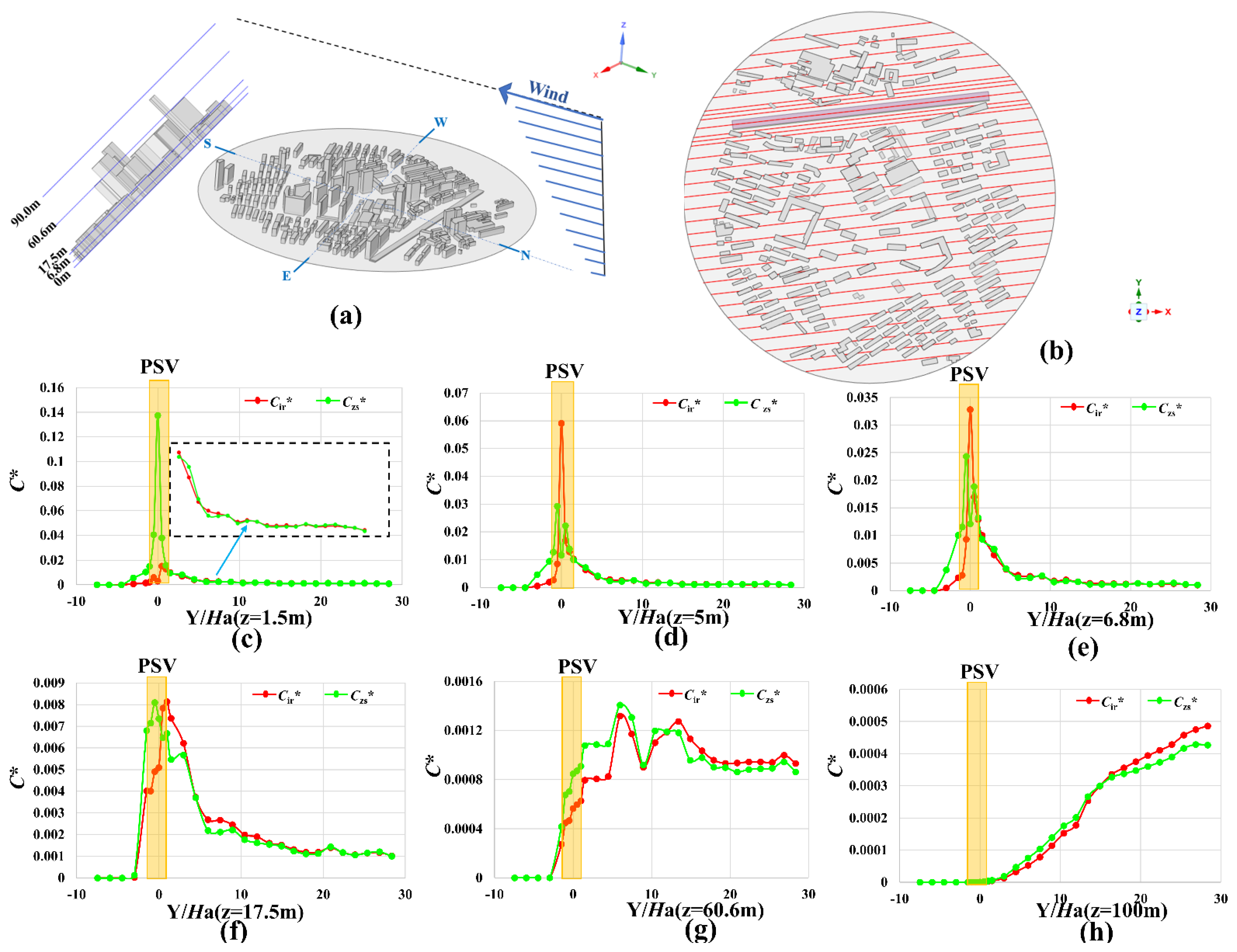
2.4. Pollutant Source Volume (PSV)

Automobile exhaust gasses were emitted near road level. This urban model had two roads: a ground–level road and an inner ring viaduct running from east to west. These two roads were treated as emitting sources. A uniform pollution source assumed to be a passive scalar was generated from 0.5–2.5 m (z) above the ground–level road and another above the inner ring viaduct 4.5–6.5 m in the z–direction, as shown in Figure 1c, to simulate pollution from vehicles. The parameter settings of each pollution source volume (PSV) are shown in Figure 1d.

3. Ventilation Efficiency and Urban form Indices

3.1. Ventilation Efficiency Indices

3.1.1. Spatially–Averaged Wind Velocity Ratio (VR_w)

The spatially–averaged wind velocity ratio (VR_w) is defined as the ratio of spatially–averaged wind velocity at the pedestrian level to a reference wind velocity [57] and is calculated as:

VR_w = U_i/U_ref

(8)

where U_i is the spatially–averaged wind speed at position i in the studied area (m/s). In this study, U_ref = 4.64 m/s.

3.1.2. Spatially–Averaged Normalized Concentration (C*)

C* is defined as the spatially–averaged normalized concentration [58] and is calculated as:

C* = (CU_refW²)/Q

(9)

where C is the calculated spatially–averaged concentration (kg/kg); W = 6.3 m; U_ref = 4.64 m/s; and Q is the pollution emission rate (m³/s). In this study, C_zs* represents the spatially–averaged normalized pollutant concentration released from the ground traffic source and C_ir* represents the spatially–averaged normalized pollutant concentration released from the viaduct traffic source.

3.2. Urban Morphological Parameters

Urban morphological characteristics directly affect the wind and near–surface turbulence in an urban microclimate and ultimately affect air quality [15,42]. In this study, urban morphological parameters closely related to the microclimate were used as indicators, such as building density (BD) [38,59], floor area ratio (FAR), average building height (AH) [60,61], spatial openness (SO), building height standard deviation (SDH), average building volume (MBV), and enclosure degree (DE). Related equations for these parameters can be found in Supplementary Materials [42].

4. Results and Discussion

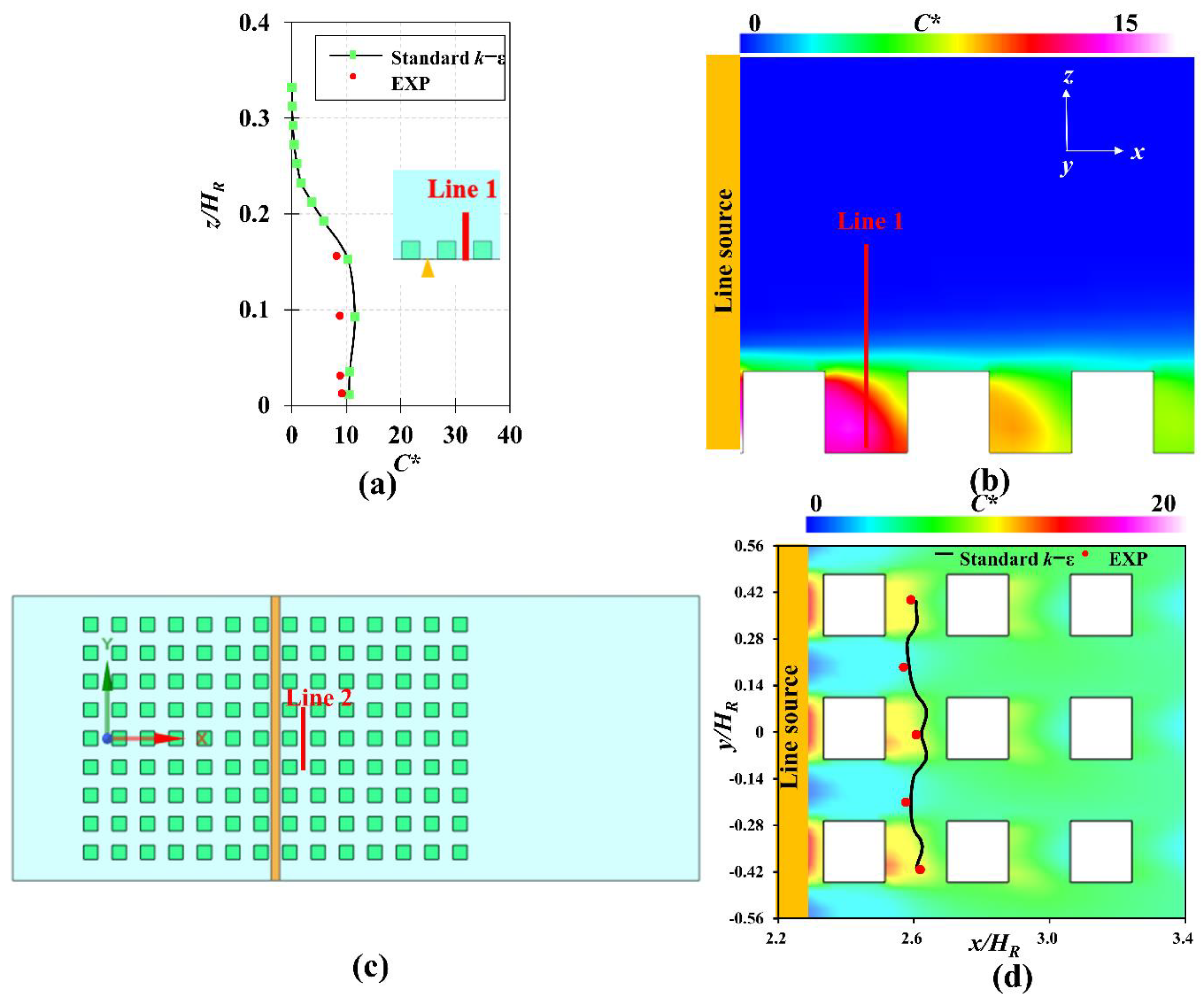
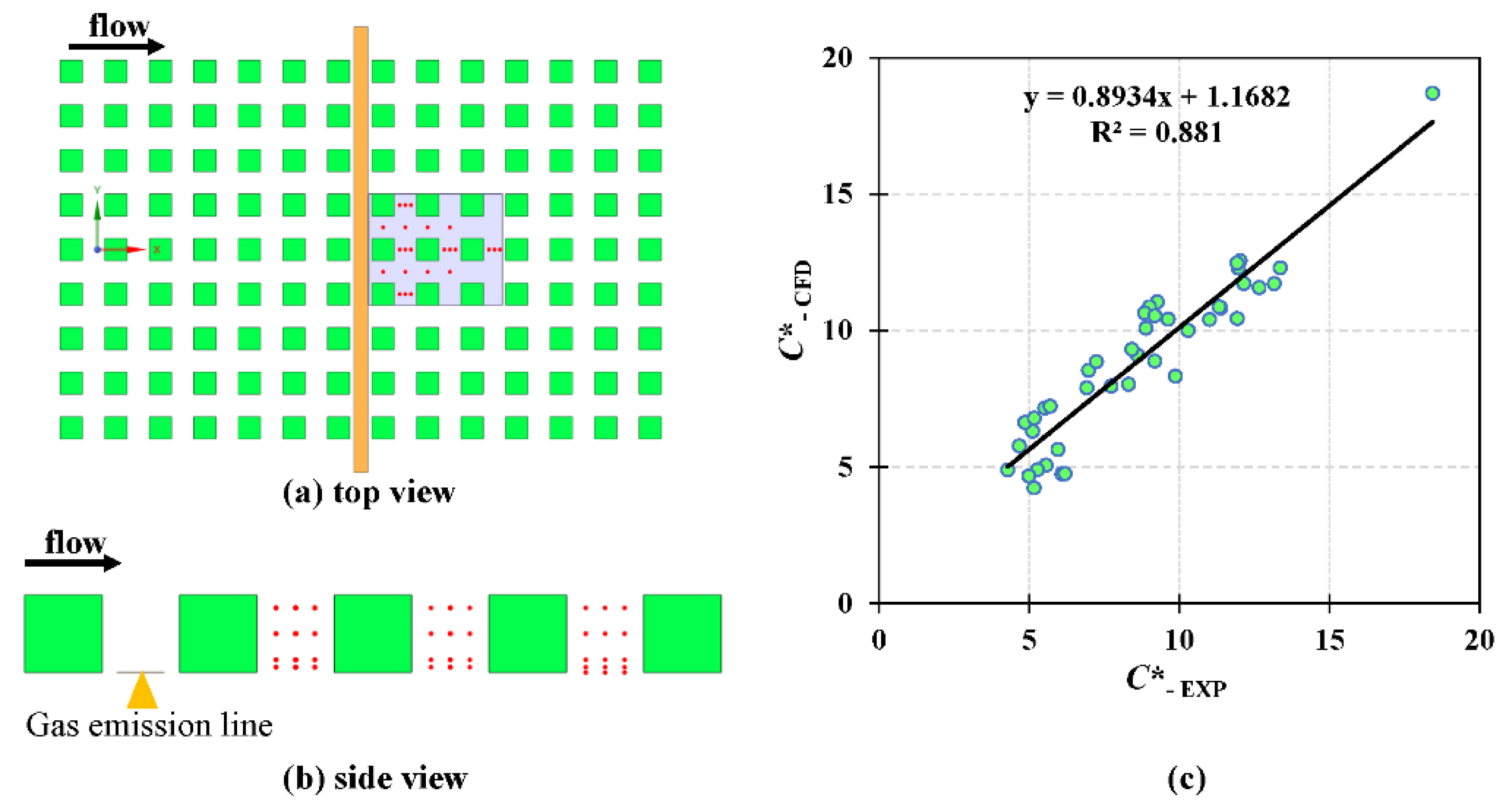
4.1. CFD Model Validation

To validate numerical simulations, wind tunnel data from [62] were used to evaluate the CFD simulations by coupling outdoor airflows of a reduced–scale urban street model (Figure 4c). CFD results were compared with wind tunnel data in Figure 4 and Figure 5. As illustrated in Figure 4, the compared positions included a vertical line (y = 0.12 m) and a horizontal line (z = 0.05 m). As displayed in Figure 4a, the vertical distributions of the calculated mean concentration and their comparisons with the mean concentration were obtained from experiments on the vertical centerline. One experimental dot shows a small vertical deviation from the CFD value. As shown in Figure 4d, the mean concentration variables obtained from CFD results correspond with the experimental data. Figure 5 compares the correlations of experimental C* and CFD C* for all the measurement positions (92 in total). The line slopes were 0.8934, and their correlation with R² reached 0.881. In order to investigate the sensitivity of grid resolution, another grid cell system (three times the original number of grid cells) was checked for the reference case (Supplementary Materials, Figure S1a). The difference between Standard $k$–$\epsilon$, Realiable $k$–$\epsilon$, and RNG $k$–$\epsilon$ model of ventilation efficiency indices was small (Supplementary Materials, Figure S1b). Overall, the CFD results (standard $k$–$\epsilon$) were satisfactory.

For this case, an unstructured polyhedral mesh of 660,000 cells was made. In order to investigate the grid resolution sensitivity, two additional grid cell systems (three times and nine times the original number of grid cells) were examined as reference cases (Supplementary Materials, Figure S1). The results showed that the difference between the three grid systems of the mean concentration variables was extremely small. We also examined the effects of the turbulence model. The difference between the Standard, Reliable, and RNG $k$–$\epsilon$ of the mean concentration variables was small. Results showed that the technique of adopting CFD simulations by standard $k$–$\epsilon$ turbulence models was effective for current research.

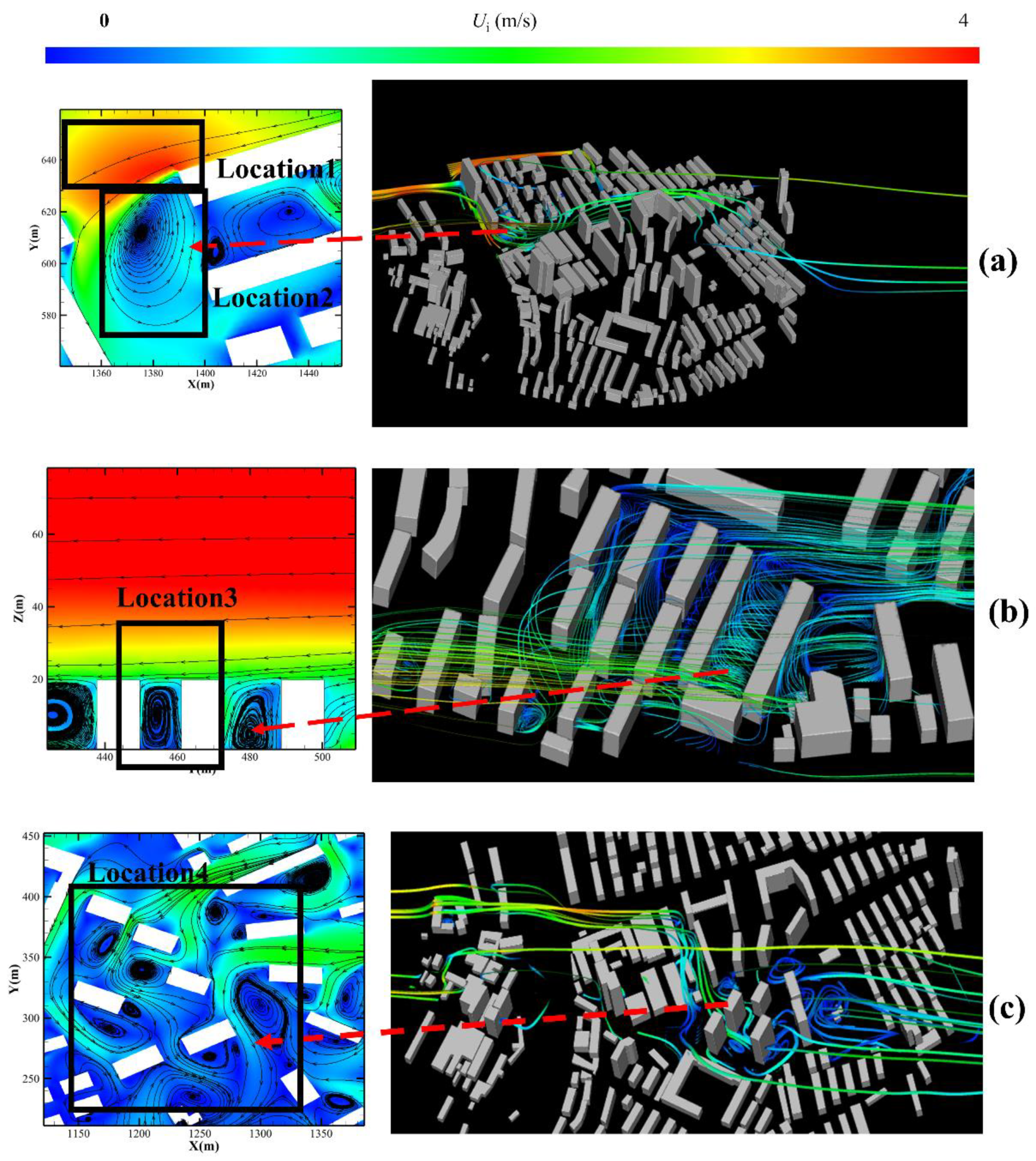
4.2. Distributions of Mean Flow Variables

We selected Z–plane = 1.5 m (pedestrian–level), 5 m (viaduct–level), 6.8 m (average height of low–rise buildings), 17.5 m (average height of multi–story buildings), 60.6 m (average height of high–rise buildings), 100 m (10 m higher than the highest building in the study area), and 150 m (no building exists), and vertical symmetry x = 1224 m (located in the center of the study area) to study the urban wind environment, pollutant concentration distribution, and other characteristics. As shown in Figure 6, the canyons were divided into two types. One was characterized by more intense ventilation (wider roads), and the other shows stagnation (e.g., downwind of a building complex, narrower roads, leeward of a building) (Figure 6c,d). Due to the low dilution process involved, these stagnant areas may result in higher pollutant concentrations. The velocity field can indicate distribution on the vertical plane. In urban areas, the extended low–speed zone and recirculation zone were located downwind of the building, as shown in Figure 6c. In a high–density environment, different building layouts produced significantly different wind environments and caused distinct changes in diffusion and flow of air pollution. However, due to the complexity of urban geometric structures, the contour plot at vertical symmetry shows that the C* inside the urban canyon was not consistent with the wind environment, as shown in Figure 7b.

Figure 8 shows the complexities and characteristics of the wind fields at different heights. Dispersion in the 3D street canyon was mainly affected by the flow structure. Figure 9 depicts the flow structure obtained from particle path lines by tracing a set of streamlines from the sides of buildings in the domain. The streamlines were colored by U_i. Under the influence of different building configurations, the airflow creates divergent effects. The concentration contour plots of Figure 7 are on six different horizontal planes (z = 1.5 m, z = 6.8 m, z = 17.5 m, z = 60.6 m, z = 100 m, and z = 150 m). The general tendencies of C* decreasing as height increases are shown in Figure 7. The urban air pollutants emanating from ground level and viaduct level show similar horizontal and vertical distribution laws of concentration.

At the pedestrian level, wind can flow into the complex from wide paths or through gaps between buildings. From Figure 6d, we observed that the main air duct determines where the C* were dispersed. The incoming winds carry a large amount of pollutants down the main road to this area. It can be observed that C* has strong non–uniformity (Figure 7c). High pollutant concentrations formed in some areas (shown in red). We also observed several special locations. At Location 1, due to its proximity to PSV, a high pollutant concentration occurred despite the high wind speed (Figure 6d). At Location 2, C* was small relative to that at Location 1. As shown in the black rectangle (Location 1) in Figure 8a, the wind–flow patterns around buildings showed flow separation, resulting in acceleration of flow around the buildings (Location 1). The VR_w at Location 2 was smaller than that at Location 1. A corner vortex was observed at Location 2. The visualizations show that the corner vortex was a recirculation of the flow behind the obstacles (shown in Figure 9a Location 2), and it has a vertical axis. The corner vortices were driven by shear at the street ends induced by channel flow. It can be concluded that a place with a higher wind speed may not always result in lower pollutant concentrations. Although a vortex forms near sources of PSV, due to the wind–flow pattern, including flow separation, pollutants rarely gather in the vortex. However, although pollutants follow the wind into Location 3 as shown in Figure 7c, a vertical vortex was formed here (shown in Figure 8b), which was conducive to the exchange of atmosphere. Thus, C* is smaller than in other surrounding places. Horizontally rotating canyon vortices were observed through the canyons (a cluster of high–rise buildings), as shown in Figure 9c. Unlike vertical vortices, this trapped, swirling air mass, while contributing to the dilution of the canyon pollution, cannot be directly ventilated through the interface between the canyon top and the atmosphere above. Canyon vortices were driven by shear forces of skimming flow over the rooftops. In the inhomogeneous urban geometry, the visualizations showed two different flow characteristics. Thus, local architectural geometry had a great influence on local ventilation patterns, and vertical vortices were more conducive to the spread of pollution.

With an increase in height, the wind speed gradually increased, and the wind field clearly changed. However, over a cluster of high–rise buildings, the wind speed was slightly weakened (black rectangle in Figure 8e). At Z–plane height = 60.6 m, there was still a high concentration of pollution in areas with a cluster of high–rise buildings. When approaching wind is interrupted by a building, wind tends to flow over and around the building, as shown in Figure 6. Therefore, in general, the upper wind speed on the leeward side of the building is higher than the lower wind speed, which drives airflow from ground level to a higher elevation. Then, eventually, it collides with the airflow above the building, weakening the wind speed at higher altitudes. This mechanism is known as the Venturi effect in urban space [63]. Due to this effect, the vertical air exchange caused by ventilation and turbulence within the city causes pollutants to be transported to altitudes of more than 60.6 m.

Small amounts of pollutants can still be found in the urban canopy, as shown in Figure 7g (no building exists). Therefore, it is also necessary to pay attention to the distribution of air pollution around high–rise buildings.

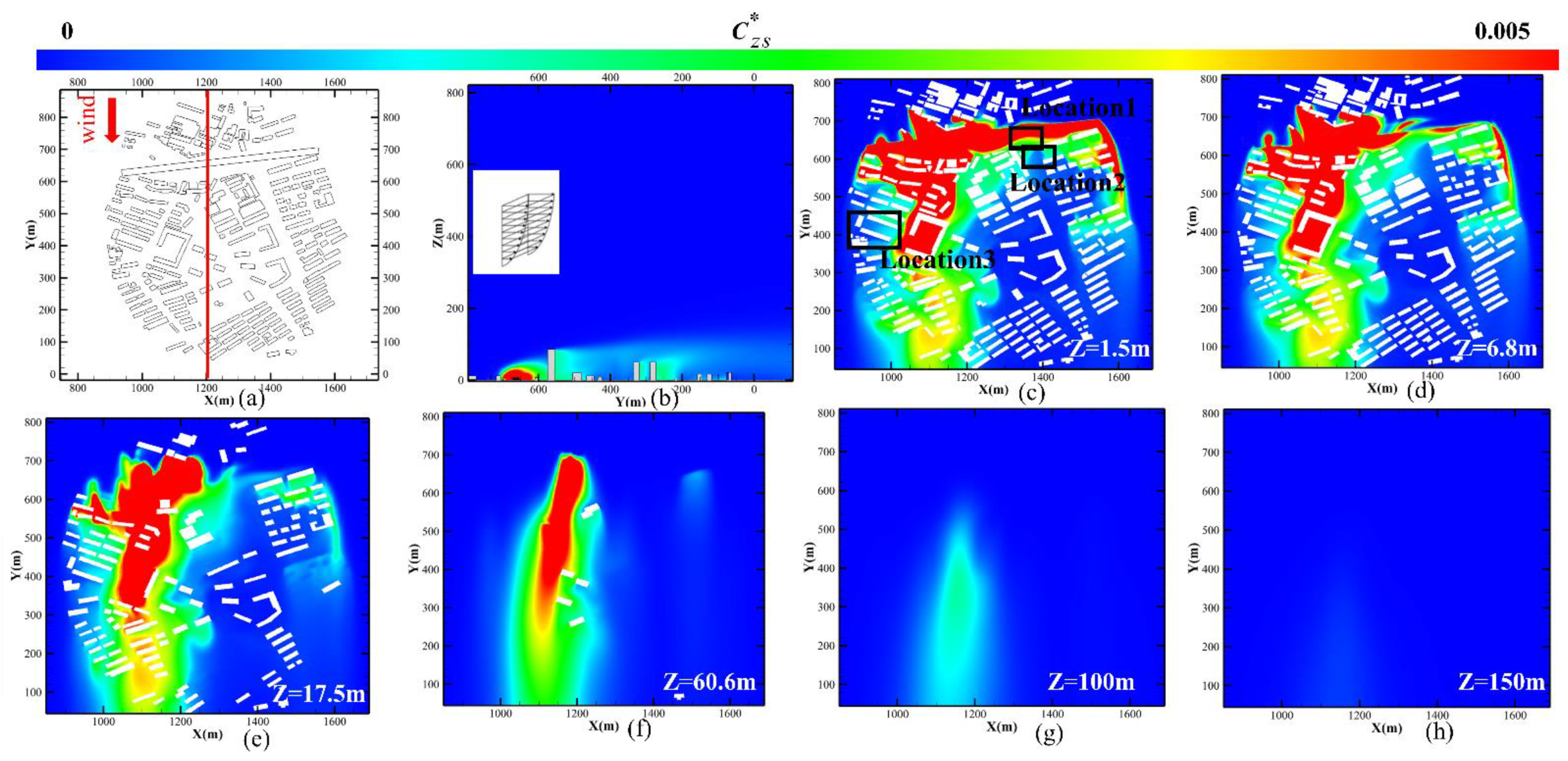
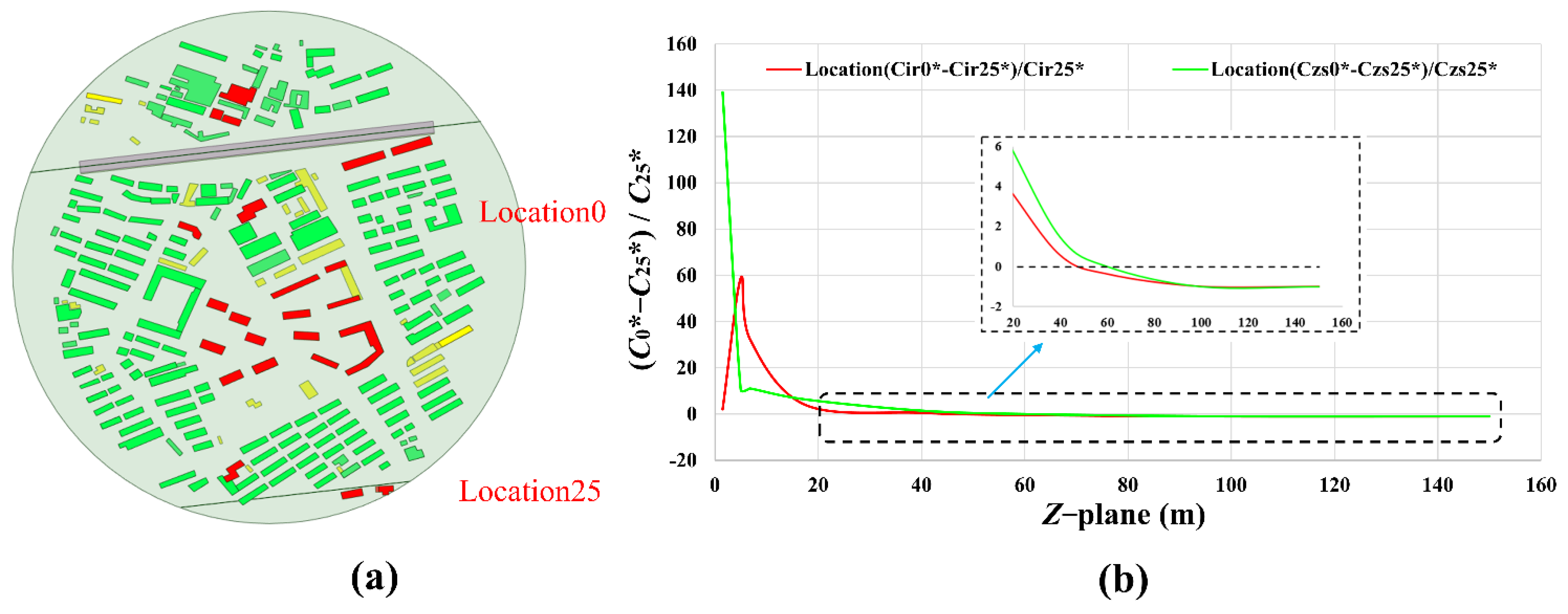
4.3. Effect of Distance from Pollutant Source Volume and Vertical Height on Normalized Pollutant Concentration (C*)

In order to study the variation of pollutant concentration with distance from the PSV, we defined the central axis position of the PSV as the centerline (Y = 0) and took three lines 10 m apart near the PSV. Then, we took the C* values in order at equal intervals of 30 m as shown in Figure 10b and finally obtained an average C* on each line.

We analyzed the variation trend of the average C* with distance at different heights and selected several representative heights, as shown in Figure 10. The variation of pollutant concentration with distance from the pollution source was inconsistent at different heights. At pedestrian level (Z–plane = 1.5 m), both upstream and downstream of the PSV, C* tended to decrease gradually with further distance, as shown in Figure 10c. Upstream of the PSV, C* released from ground sources showed a greater rate of change. Downstream of the PSV, the C* released from the viaduct and ground showed similar variation trends. C* decreased rapidly within 50 m of the PSV, then, with further increase in distance, the trend of change became gentle. Meanwhile, it can be observed that the buildings upstream of the pollution source are more seriously polluted by urban air pollutants released at ground level. At Z–planes = 5 m, 6.5 m, and 17.5 m, we observed that the variation trend of pollutant concentration was similar to that at pedestrian height in Figure 10d–f. As height increases, the variation trend of pollutant concentration with distance presents an anomaly.

Location 0 (the central axis location of PSV) and location 25 (600 m from PSV) were selected in Figure 11 to analyze the variation of traffic–related pollutant dispersion with heights from the source to downstream. The difference between the C* values at location 0 and location 25 was compared to C* at location 25. If the resulting value > 0, it means that the pollutant concentration at location 0 was greater than that at location 25. If the resulting value = 0, it means that the pollutant released by PSV was diffused downstream in equal amounts. If the resulting value < 0, it means that the C* released by PSV diffused downstream in large quantities. As shown in Figure 11, C* at Location 0 was 139 times higher than that at Location 25, until the C_zs* values at the two locations reached the same level at about 60 m in the Z–plane plan. C* at Location 0 was lower than that at Location 25. Urban air pollutants C* increased irregularly with an increase in distance at Z–planes = 60.6~86 m, as shown in Figure 10g, and the two high–value points of C* both appeared in the area with high–rise buildings. This observation was linked to the characteristics of ventilation flow described in Section 4.2. Above 86 m in Z–plane, as shown in Figure 10h, the C* values tended to increase linearly with further distance.

In order to further quantitatively describe the contribution of ground pollution sources and viaduct pollution sources at different block heights, area–weighted averages of concentrations of the two pollutants on the cross–sections at different heights were calculated. Figure 12 shows the averaged cross–section C* at ground level and viaduct level at different heights.

The pollutants released at the ground level reached their maximum concentrations at Z–plane = 2.5 m, and the pollutants released at viaduct level reached their maximum concentrations at Z–plane = 8 m. By comparing their contribution rates at different heights, it can be found that the urban air pollutants released at ground level were dominant when the Z–plane was below 8 m high, while the pollution concentration released by the viaduct source was about 0.8–6.1% higher than that released by the ground source when the Z–plane was above 8 m high. At Z–plane heights = 5 m, 6 m, the pollutant concentration from the ground–source decreased by about 33% compared with that at Z–plane height = 4 m. The elevated road acted such as a hat, preventing the upward transport of pollutants emitted by ground–level traffic, resulting in a sudden decrease in pollutant concentrations within this range. In addition, although the pollution released from the viaduct level was generally located at the height of 4.5 m in the city, the contribution rate of urban air pollutants released from ground level at this height was still large. It is worth noting that, in the height range of Z–plane = 2.5–4.5 m, the superposition effect of the two was the largest, and this has the greatest impact on residents’ health.

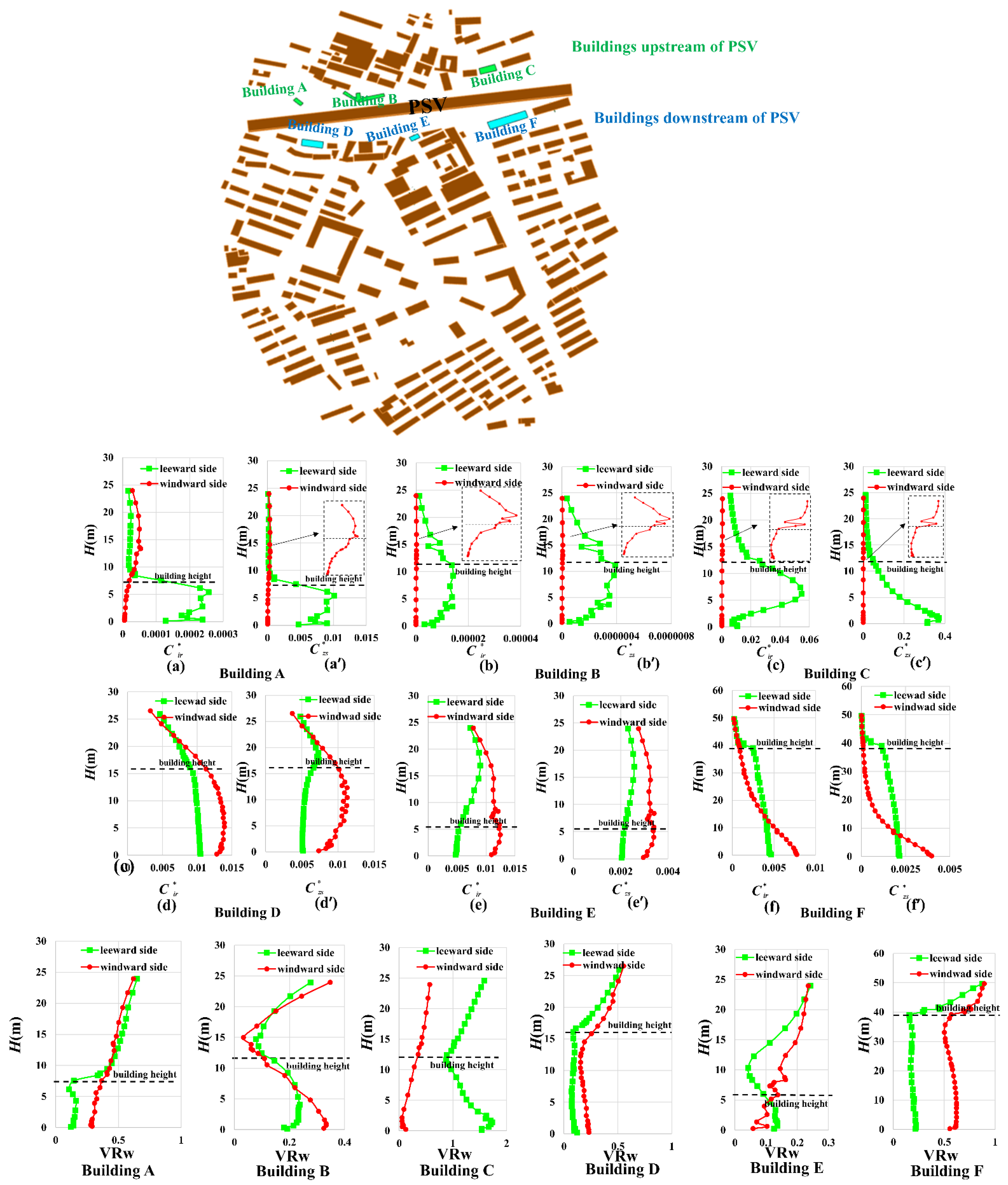
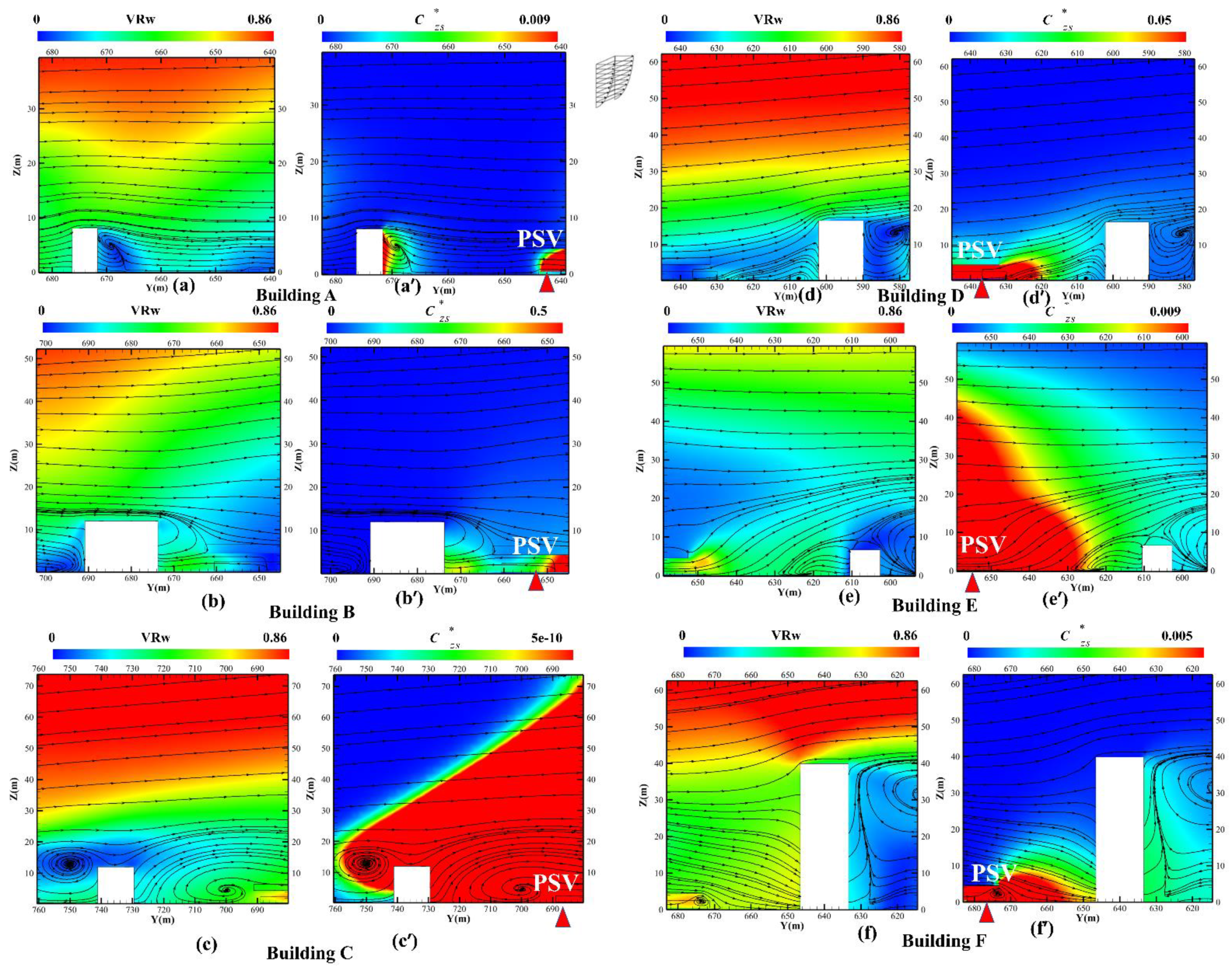
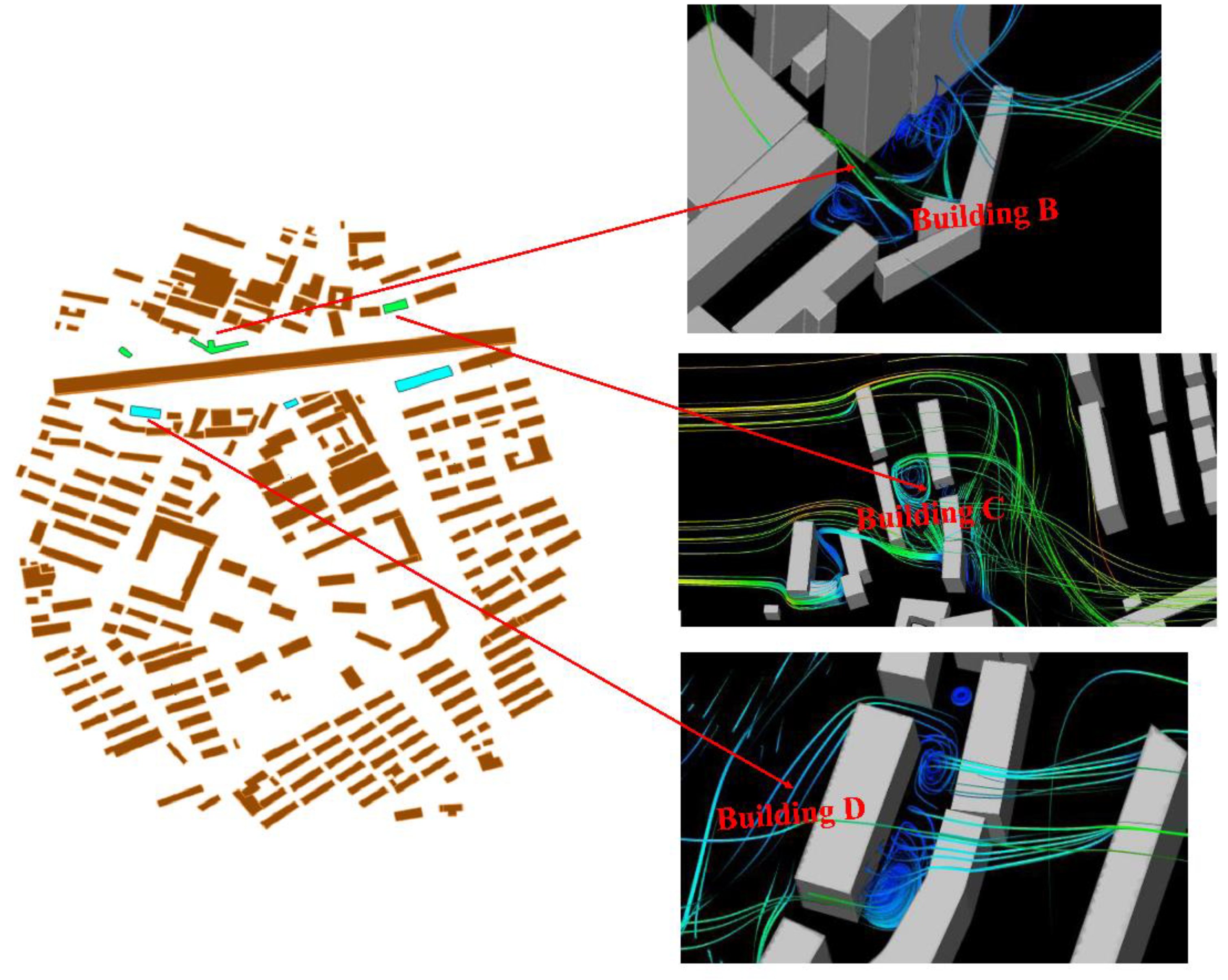
4.4. Vertical Distribution of Air Pollutant Concentration around Typical Buildings

In order to study the variation of pollutants concentrations around high buildings, six buildings, A, B, C, D, E, and F, on both sides of the road were selected for analysis. Their selection was based on the following considerations: those buildings facing the street are close to PSV. They are of three types: low–rise, multi–story, and high–rise. Therefore, it is of great significance to study the vertical variation of pollutants near the street. We extracted data from 1 m from the buildings to analyze the variation of C* and VR_w on the windward and leeward sides with building height.

Figure 13 shows the windward and leeward sides C* (vertical variation of average concentration across the profile). Target buildings A, B, and C were located upstream of PSV. The C* on the windward side of the building increased gradually with the building height. This is due to the observation that downwind of the building, the pollutants emitted from PSV are carried back to the windward side by gyratory air currents and accumulate mainly upstream of the building, as shown in Figure 14a′–c′. However, there are various trends on the building’s leeward side. C* repeatedly increases and then decreases with the height of building A (Figure 13a,a′). Due to the shading of the building itself, a lower wind speed zone was observed on the leeward side of building A (Figure 14a), allowing a significant accumulation of pollutants here. The C* on the leeward side of building B increased gradually with building height. It is worth noting that the vertical variation of pollutants varies for different pollution sources (Figure 12 building B). On the leeward side of building C, due to the complex wind structure characteristics on the leeward side of building C (Figure 14), as shown in Figure 13c, the leeward–side wind structure of Building C has complex wind structure characteristics and a vertical clockwise vortex brings pollutants back near Building C. At the same time, the elevated and ground–level release of pollutants are at different heights, and the concentration of pollutants brought back down the vortex is not the same. Therefore, the height of maximum C* for different pollution sources and the trend of change with height was completely different. Besides, the C* on the leeward side of the building was about twice that on the windward side.

Target buildings D, E, and F are located downstream of PSV. The C* on the windward side of buildings D and E first increase and then decrease with building height. The windward sides of buildings D and E have the same wind environment characteristics, with the incoming winds separating into upward and downward flow patterns at the top of the building. Thus, pollutants reach their maximum concentrations in the middle section (Figure 14d,e). On the leeward side of building D, C* released from the viaduct source gradually decreased with building height (Figure 13d), while C* released from the ground source slowly increased with building height (Figure 13d′). The leeward side C* of building E showed no obvious change trend with building height. Meanwhile, the C* on the windward side of buildings D and E were greater than those on the leeward side. However, the VR_w on the windward side of building D was greater than that on the leeward side, and that on the windward side of building E was smaller than that on the leeward side. Building F is a high–rise building. The C* values on the windward and leeward sides decreased gradually with building height, and the variations of C* values on the windward side and the leeward side intersect at the height of about 10 m. The C* on the leeward side was higher than that on the windward side when the height is above about 10 m. The underlying cause of this is the formation of a vertical counterclockwise vortex on the upper part of the leeward side of building F (as shown in Figure 14f). Overall, vertical profiles of C* were building specific, and its change rate was inconsistent with height increase. At the same time, the C* values on the leeward sides of the buildings upstream of PSV were higher than those on the windward sides, while the C* values on the buildings downstream of PSV showed the opposite pattern. These results were mainly related to the complex flow patterns around the buildings.

The relationships between C* and VR_w on the leeward side and between C* and KE_turb on the windward side of the building are as shown in

Table 2. Analysis on Spearman correlation coefficients among VR_w/C_zs*, C_ir*.

r/R2		Leeward		Windward
Buildings		Cir*	Czs*	Cir*	Czs*
A	VRw	−0.793/0.629	−0.796/0.634	0.992/0.984	0.992/0.984
B	VRw	−0.700/0.490	0.992/0.984	0.864/0.746	0.862/0.743
C	VRw	0.097/0.009	−0.084/0.007	−0.981/0.963	−0.981/0.962
D	VRw	−0.145/0.021	0.278/0.078	−0.546/0.298	−0.677/0.458
E	VRw	−0.964/0.929	−0.962/0.925	0.618/0.382	0.754/0.568
F	VRw	0.866/0.751	0.839/0.704	0.754/0.568	0.633/0.401

and

Table 3. Analysis on Spearman correlation coefficients among KE_turb/C_zs*, C_ir*.

r/R2		Leeward		Windward
Buildings		Cir*	Czs*	Cir*	Czs*
A	KEturb	−0.690/0.476	−0.670/0.449	−0.866/0.751	−0.866/0.751
B	KEturb	0.531/0.282	−0.941/0.886	0.051/0.003	0.051/0.003
C	KEturb	0.563/0.465	0.682/0.317	0.923/0.857	0.926/0.857
D	KEturb	−0.949/0.901	0.983/0.881	−0.757/0.574	0.597/0.356
E	KEturb	0.803/0.645	0.813/0.660	0.800/0.629	0.920/0.847
F	KEturb	−0.967/0.822	−0.900/0.802	−0.842/0.709	−0.751/0.564

, respectively. Except for buildings C and D, VR_w and C* were highly correlated (maximum R² = 0.992). The leeward side of building C had a wider space where the wind can be directly injected. Meanwhile, two vortices were observed on the leeward side of Building D (Figure 15), which resulted in no significant correlation between VR_w and C*. Even though we were analyzing at the same location, the correlations between C* and VR_w were different for different PSV (such as buildings C).

Except for buildings B (windward side) and C, KE_turb, and C* were highly correlated (maximum R² = 0.920). Due to the irregular shape of building B, the wind splits into two streams and produces vortices, which may be the reason for its low correlation. In general, the correlations between C* and VR_w and between C* and KE_turb were greater for the windward sides of the PSV upstream buildings than for the leeward sides and the buildings downstream of the PSV showed the opposite situation.

4.5. Effect of Urban Morphological Parameters on Ventilation Efficiency Indices

In order to study the correlations between urban parameter factors and ventilation indices, we first divided the research area into 29 plots according to the community’s urban texture and boundary (Figure 16). Then, 7 urban parameter factors (described in Section 3.2) and the area–weighted averages of ventilation indices (VR_w, C_ir* and C_zs*) in each area at pedestrian level (Z–plane = 1.5 m) were calculated, and the correlation between them was analyzed.

As shown in

Table 4. Analysis of morphological variables, VR_w, C_ir* and C_zs*.

Test Parameters		R	R2	Adjusted R2	F Ratio	p-Value
BD	VRw	0.251	0.023	0.029	1.822	0.188
	Cir*	0.066	0.004	−0.032	0.119	0.194
	Czs*	0.064	0.004	−0.033	0.111	0.742
FAR	VRw	0.210	0.044	0.009	1.245	0.274
	Cir*	0.116	0.013	−0.023	0.365	0.551
	Czs*	0.266	0.071	0.037	2.063	0.162
SO	VRw	0.020	0.0003	−0.037	0.011	0.918
	Cir*	0.072	0.005	−0.032	0.139	0.712
	Czs*	0.002	3.083 × 10−6	−0.037	8.325 × 10−5	0.993
AH	VRw	0.056	0.003	−0.034	0.085	0.773
	Cir*	0.165	0.027	−0.009	0.753	0.393
	Czs*	0.201	0.040	0.005	1.134	0.296
SDH	VRw	0.127	0.016	−0.020	0.443	0.511
	Cir*	0.071	0.005	−0.032	0.137	0.714
	Czs*	0.170	0.029	−0.007	0.799	0.379
MBV	VRw	0.108	0.012	−0.025	0.321	0.576
	Cir*	0.149	0.022	−0.014	0.611	0.441
	Czs*	0.216	0.047	0.011	1.322	0.260
DE	VRw	0.059	0.004	−0.033	0.095	0.760
	Cir*	0.112	0.013	−0.024	0.344	0.563
	Czs*	0.168	0.028	−0.008	0.781	0.385

, there does not seem to be a strong correlation between the 7 urban form factors and 3 ventilation indices (p > 0.1). This was inconsistent with the conclusions drawn in some previous works. We also found that there did not seem to be a strong correlation between urban form factors and ventilation factors. This was also inconsistent with some conclusions drawn by previous researchers using idealized blocks and relatively uniform actual blocks [11,15,38,42]. The main reason for this may be that an actual block was used in this study and its architectural form and arrangement were different. Therefore, in a later work, it will be necessary to design more urban blocks and to consider factors such as different wind angles to enrich the study of the correlation between urban form factors and ventilation factors.

5. Conclusions

CFD simulations using the standard $k$–$\epsilon$ model were carried out to evaluate airflows and traffic–related air pollution distributions in a real urban area. The boundary conditions of the inflow were based on statistical data of long–term observations by a weather station in the target area. The dual effects of surface road pollution sources and elevated road pollution sources on the air quality of the urban area were considered at the same time. Two ventilation efficiency indices (including spatially–averaged wind speed ratio (VR_w) and normalized pollutant concentration (C*) were adopted. The results of this research will be helpful in the investigation of the migration of urban pollutants and of great significance to the construction of green cities and the unification of architecture and environmental science. The main conclusions are as follows:

(1)

Buildings in urban areas affect wind environments in different aspects such as urban form characteristics, architectural forms, and building heights. Urban ventilation is mainly affected by two flow characteristics: vertically rotating canyon vortices and horizontally rotating corner vortices. Local architectural geometry has a great influence on local ventilation patterns. Furthermore, wind flows near low– to medium–rise buildings indicate complicated wind–building interactions, which may be responsible for the complex air ventilation assessment results in urban areas.

(2)

Later, the effect of distance from PSV on C* was investigated. From ground level to a height of 60 m, C* tends to decrease gradually with distance from PSV. C* increases irregularly with an increase in distance between 60 m and 86 m, and two high–value points of C* appear in an area with high–rise buildings. Above 86 m, C* tends to increase linearly with further distance.

(3)

In a study of the effect of vertical height on C* it was found that: C* generally decreases with height. Based on the comparison of pollutant contribution rates of two kinds of pollutant sources (ground–level and viaduct–level) at different heights, it is shown that ground sources release 2.9 times more pollutants than viaduct sources at Z–plane = 2.5 m. It was also found that pollutants released by ground–level sources are dominant when the Z–plane is below 8 m high, and pollutants released from viaduct sources are about 0.8–6.1% higher when the Z–plane is above 8 m high.

(4)

Quantitative vertical analyses were conducted of C* on the windward and leeward sides of buildings upstream and downstream of the street. Overall, vertical profiles of pollutant concentration were building–specific, and their rates of change were inconsistent with height increases. At the same location, correlations between C* and VR_w were different for different PSV. In general, the correlation between C* and VR_w and between C* and KE_turb was greater for the windward side of the PSV upstream buildings than for the leeward side. Buildings downstream of the PSV showed the opposite situation.

(5)

Lastly, the correlation between urban parameter factors and ventilation indices were investigated at the pedestrian level. The 7 urban morphological parameters selected in this study showed no significant correlation with VR_w, C_ir* and C_zs*.

References

1. United Nations, Department of Economic and Social Affairs, Population Division. World Urbanization Prospects. 2018. Available online: www.un.org/development/desa/pd/themes/urbanization (accessed on 25 October 2021).
2. United Nations. Policies on Spatial Distribution and Urbanization Have Broad Impacts on Sustainable Development. 2020. Available online: https://www.un.org/development/desa/pd/sites/www.un.org.development.desa.pd/files/undes_pd_2020_popfacts_urbanization_policies.pdf (accessed on 26 October 2021).
3. Shanghai Municipal Statistics. Shanghai Statistical Yearbook. 2020. Available online: http://tjj.sh.gov.cn/tjnj/20210303/2abf188275224739bd5bce9bf128aca8.html (accessed on 20 April 2021).
4. Wang, Y.; Yao, L.; Xu, Y.; Sun, S.; Li, T. Potential heterogeneity in the relationship between urbanization and air pollution, from the perspective of urban agglomeration. J. Clean. Prod. 2021, 298, 126822. [Google Scholar] [CrossRef]
5. Ulpiani, G. On the linkage between urban heat island and urban pollution island: Three-decade literature review towards a conceptual framework. Sci. Total Environ. 2021, 751, 141727. [Google Scholar] [CrossRef] [PubMed]
6. Sun, D.J.; Shi, X.; Zhang, Y.; Zhang, L. Spatiotemporal distribution of traffic emission based on wind tunnel experiment and computational fluid dynamics (CFD) simulation. J. Clean. Prod. 2020, 282, 124495. [Google Scholar] [CrossRef]
7. Vardoulakis, S.; Fisher, B.E.A.; Pericleous, K.; Gonzalez-Flesca, N. Modelling air quality in street canyons: Review. Atmos. Environ. 2003, 37, 155–182. [Google Scholar] [CrossRef] [Green Version]
8. Buccolieri, R.; Salim, S.M.; Leo, L.S.; Di Sabatino, S.; Chan, A.; Ielpo, P.; de Gennaro, G.; Gromke, C. Analysis of local scale tree–atmosphere interaction on pollutant concentration in idealized street canyons and application to a real urban junction. Atmos. Environ. 2011, 45, 1702–1713. [Google Scholar] [CrossRef]
9. Wang, X.; Yang, X.; Wang, X.; Zhao, J.; Hu, S.; Lu, J. Effect of reversible lanes on the concentration field of road-traffic-generated fine particulate matter (PM2.5). Sustain. Cities Soc. 2020, 62, 102389. [Google Scholar] [CrossRef]
10. Xin, Y.L.; Shao, S.Q.; Wang, Z.C.; Xu, Z.W.; Li, H. COVID-2019 Lockdown in Beijing: A Rare Opportunity to Analyze the Contribution Rate of Road Traffic to Air Pollutants. Sustain. Cities Soc. 2021, 75, 102989. [Google Scholar] [CrossRef]
11. Yuan, M.; Song, Y.; Huang, Y.; Shen, H.; Li, T. Exploring the association between the built environment and remotely sensed PM2.5 concentrations in urban areas. J. Clean Prod. 2019, 220, 1014–1023. [Google Scholar] [CrossRef]
12. Chang, D.; Song, Y.; Liu, B. Visibility trends in six megacities in China 1973–2007. Atmos. Res. 2009, 94, 161–167. [Google Scholar] [CrossRef]
13. Quan, J.; Zhang, Q.; He, H.; Liu, J.; Huang, M.; Jin, H. Analysis of the formation of fog and haze in North China Plain (NCP). Atmos. Chem. Phys. 2011, 11, 8205–8214. [Google Scholar] [CrossRef] [Green Version]
14. Wu, J.; Fu, C.B.; Zhang, L.Y.; Tang, J.P. Trends of visibility on sunny days in China in the recent 50 years. Atmos. Environ. 2012, 55, 339–346. [Google Scholar] [CrossRef]
15. Edussuriya, P.; Chan, A.; Ye, A. Urban morphology and air quality in dense residential environments in Hong Kong. Part I: District-level analysis. Atmos. Environ. 2011, 45, 4789–4803. [Google Scholar] [CrossRef]
16. Santiago, J.L.; Martin, F. Use of CFD modeling for estimating spatial representativeness of urban air pollution monitoring sites and suitability of their locations. Física Dela Tierra 2015, 27, 191. [Google Scholar]
17. Deng, X.; Li, F.; Li, Y.; Li, J.; Huang, H.; Liu, X. Vertical distribution characteristics of PM in the surface layerof Guangzhou. Particuology 2014, 20, 3–9. [Google Scholar] [CrossRef]
18. Han, S.; Bian, H.; Tie, X.; Xie, Y.; Sun, M.; Liu, A. Impact of nocturnal planetary boundary layer on urban air pollutants: Measurements from a 250-m tower over Tianjin, China. J. Hazard. Mater. 2009, 162, 264–269. [Google Scholar] [CrossRef] [PubMed]
19. Sun, Y.; Wang, Y.; Zhang, C. Measurement of the vertical profile of atmospheric SO2 during the heating period in Beijing on days of high air pollution. Atmos. Environ. 2009, 43, 468–472. [Google Scholar]
20. Fan, S.H.; Gao, C.Y.; Yang, Y.J.; Liu, Z.; Hu, B.; Wang, Y.; Wang, J.; Gao, Z. Elucidating roles of near-surface vertical layer structure in different stages of PM2.5 pollution episodes over urban Beijing during 2004–2016. Atmos. Environ. 2020, 246, 118157. [Google Scholar] [CrossRef]
21. Peng, Z.R.; Wang, D.S.; Wang, Z.Y.; Gao, Y.; Lu, S.J. A study of vertical distribution patterns of PM2.5 concentrations based on ambient monitoring with unmanned aerial vehicles: A case in Hangzhou, China. Atmos. Environ. 2015, 123, 357–369. [Google Scholar] [CrossRef]
22. Li, X.; Leung, D.Y.C.; Liu, C.H.; Lam, K.M. Physical modeling of flow field inside urban street canyons. J. Appl. Meteorol. Climatol. 2008, 47, 2058–2067. [Google Scholar] [CrossRef]
23. Yassin, M.F. A wind tunnel study on the effect of thermal stability on flow and dispersion of rooftop stack emissions in the near wake of a building. Atmos. Environ. 2013, 65, 89–100. [Google Scholar] [CrossRef]
24. Gromke, C. A vegetation modeling concept for building and environmental aerodynamics wind tunnel tests and its application in pollutant dispersion studies. Environ. Pollut. 2011, 159, 2094–2099. [Google Scholar] [CrossRef] [PubMed]
25. Murakami, S.; Mochida, A.; Sakamoto, S. Numerical study on velocity-pressure field and wind forces for bluff bodies by κ-ϵ, ASM and LES. J. Wind Eng. Ind. Aerod. 1992, 44, 2841–2852. [Google Scholar] [CrossRef]
26. Tominaga, Y.; Mochida, A.; Yoshie, R.; Kataoka, H.; Nozu, T.; Yoshikawa, M.; Shirasawa, T. AIJ guidelines for practical applications of CFD to pedestrian wind environment around buildings. J. Wind Eng. Ind. Aerod. 2008, 96, 1749–1761. [Google Scholar] [CrossRef]
27. Blocken, B.; Carmeliet, J.; Stathopoulos, T. CFD evaluation of wind speed conditions in passages between parallel buildings-effect of wall-function roughness modifications for the atmospheric boundary layer flow. J. Wind Eng. Ind. Aerodyn. 2007, 95, 941–962. [Google Scholar] [CrossRef]
28. Blocken, B. 50 years of computational wind engineering: Past, present and future. J. Wind Eng. Ind. Aerodyn. 2014, 129, 69–102. [Google Scholar] [CrossRef]
29. Tamura, Y.; Xu, X.D.; Yang, Q.S. Characteristics of pedestrian-level Mean wind speed around square buildings: Effects of height, width, size and approaching flow profile. J. Wind Eng. Ind. Aerodyn. 2019, 192, 74–87. [Google Scholar] [CrossRef]
30. Xie, X.M.; Liu, C.H.; Leung, D.Y.C. Impact of building facades and ground heating on wind flow and pollutant transport in street canyons. Atmos. Environ. 2007, 41, 9030–9049. [Google Scholar] [CrossRef]
31. Xie, X.M.; Huang, Z.; Wang, J.S. Impact of building configuration on air quality in street canyon. Atmos. Environ. 2005, 39, 4519–4530. [Google Scholar] [CrossRef]
32. Cheng, W.C.; Liu, C.H.; Leung, D.Y.C. On the correlation of air and pollutant exchange for street canyons in combined wind-buoyancy-driven flow. Atmos. Environ. 2009, 43, 3682–3690. [Google Scholar] [CrossRef]
33. Liu, C.H.; Wong, C.C.C. On the pollutant removal, dispersion, and entrainment over two-dimensional idealized street canyons. Atmos. Res. 2014, 135, 128–142. [Google Scholar] [CrossRef] [Green Version]
34. Mei, S.H.; Luo, Z.W.; Zhao, F.Y.; Wang, H.Q. Street canyon ventilation and airborne pollutant dispersion: 2-D versus 3-D CFD simulations. Sustain. Cities Soc. 2019, 50, 101700. [Google Scholar] [CrossRef]
35. Hang, J.; Luo, Z.; Wang, X.; He, L.; Wang, B.; Zhu, W. The influence of street layouts and viaduct settings on daily carbon monoxide exposure and intake fraction in idealized urban canyons. Environ. Pollut. 2016, 220, 72–86. [Google Scholar] [CrossRef] [PubMed]
36. da Silva, F.T.; Reis, N.C., Jr.; Santos, J.M.; Goulart, E.V.; de Alvarez, C.E. The impact of urban block typology on pollutant dispersion. J. Wind Eng. Ind. Aerod. 2021, 210, 104524. [Google Scholar] [CrossRef]
37. Mei, S.J.; Hu, J.T.; Liu, D.; Zhao, F.Y.; Li, Y.; Wang, Y.; Wang, H.Q. Wind driven natural ventilation in the idealized building block arrays with multiple urban morphologies and unique package building density. Build. Environ. 2017, 92, 152–166. [Google Scholar] [CrossRef]
38. Hu, T.; Yoshie, R. Indices to evaluate ventilation efficiency in newly-built urban area at pedestrian level. J. Wind Eng. Ind. Aerod. 2013, 112, 39–51. [Google Scholar] [CrossRef]
39. Hang, J.; Sandberg, M.; Li, Y.G. Pollutant dispersion in idealized city models with different urban morphologies. Atmos. Environ. 2009, 43, 6011–6025. [Google Scholar] [CrossRef]
40. Di Sabatino, S.; Buccolieri, R.; Pulvirenti, B.; Britter, R. Simulations of pollutant dispersion within idealised urban-type geometries with CFD and integral models. Atmos. Environ. 2007, 41, 8316–8329. [Google Scholar] [CrossRef]
41. Hang, J. Wind Conditions and City Ventilation in Idealized City Models. Ph.D. Thesis, The University of Hong Kong, Hong Kong, China, 2009. [Google Scholar]
42. Jiang, Z.W.; Cheng, H.M.; Zhang, P.H.; Kang, T.F. Influence of urban morphological parameters on the distribution and diffusion of air pollutants: A case study in China. J. Environ. Sci. 2021, 105, 163–172. [Google Scholar] [CrossRef]
43. Hang, J.; Li, Y.G.; Buccolieri, R.; Sabatino, S.D. The influence of building height variability on pollutant dispersion and pedestrian ventilation in idealized high-rise urban areas. Build. Environ. 2012, 56, 346–360. [Google Scholar] [CrossRef]
44. Zhang, C.F.; Wen, M.; Zeng, J.R.; Zhang, G.L.; Fang, H.P.; Li, Y. Modeling theimpact of the viaduct on particles dispersion from vehicle exhaust in street canyons. Sci. China Technol. Sci. 2012, 55, 48–55. [Google Scholar] [CrossRef]
45. Hang, J.; Xian, Z.; Wang, D.; Mak, C.M.; Wang, B.; Fan, Y. The impacts of viaduct settings and street aspect ratios on personal intake fraction in three-dimensional urban-like geometries. Build. Environ. 2018, 143, 138–162. [Google Scholar] [CrossRef]
46. Michioka, T.; Takimoto, H.; Sato, A. Large-eddy simulation of pollutant removal from a three-dimensional street canyon. Bound. Layer Meteorol. 2014, 150, 259–275. [Google Scholar] [CrossRef]
47. Assimakopoulos, V.D.; ApSimon, H.M.; Moussiopoulos, N. A numerical study of atmospheric pollutant dispersion in different two-dimensional street canyon configurations. Atmos. Environ. 2003, 37, 4037–4049. [Google Scholar] [CrossRef]
48. Huang, Y.D.; Hu, X.N.; Zeng, N.B. Impact of wedge-shaped roofs on airflow and pollutant dispersion inside urban street canyons. Build. Environ. 2009, 44, 2335–2347. [Google Scholar] [CrossRef]
49. Baik, J.J.; Kim, J.J. A numerical study of flow and pollutant dispersion characteristics in urban street canyons. J. Appl. Meteorol. 1999, 38, 1576–1589. [Google Scholar] [CrossRef]
50. Xie, X.; Huang, Z.; Wang, J. The impact of urban street layout on local atmospheric environment. Build. Environ. 2006, 41, 1352–1363. [Google Scholar]
51. Garmory, P.A.; Ketzel, M.; Berkowicz, R.; Britter, R. Comparative study of measured and modelled number concentrations of nanoparticles in an urban street canyon. Atmos. Environ. 2009, 43, 949–958. [Google Scholar]
52. Jiang, G.Y.; Hu, T.T.; Yang, H.K. Effects of Ground Heating on Ventilation and Pollutant Transport in Three-Dimensional Urban Street Canyons with Unit Aspect Ratio. Atmosphere 2019, 10, 286. [Google Scholar] [CrossRef] [Green Version]
53. Li, Y.; Stathopoulos, T. Numerical evaluation of wind-induced dispersion of pollutants around a building. J. Wind Eng. Ind. Aerodyn. 1997, 67–68, 757–766. [Google Scholar] [CrossRef]
54. Peric, M.; Ferguson, S. The advantage of polyhedral meshes. Dynamics 2005, 24, 45. [Google Scholar]
55. Franke, J.; Hellsten, A.; Schlünzen, H.; Carissimo, B. Best Practice Guideline for the CFD Simulation of Flows in the Urban Environments. Tech. Rep. COST Action 2007, 732. [Google Scholar]
56. Ma, T.; Duan, F.; He, K.; Qin, Y.; Tong, D.; Geng, G.; Liu, X.; Li, H.; Yang, S.; Ye, S.; et al. Air pollution characteristics and their relationship with emissions and meteorology in the Yangtze River Delta region during 2014–2016. J. Environ. Sci. 2019, 83, 8–20. [Google Scholar] [CrossRef] [PubMed]
57. Ng, E. Air ventilation assessment for high density city-an experience from Hongkong. In Proceedings of the Seventh International Conference on Urban Climate, Yokohama, Japan, 29 June–3 July 2009. [Google Scholar]
58. Huang, H.; Ooka, R.; Kato, S.; Jiang, T. CFD analysis of ventilation efficiency around an elevated highway using visitation frequency and purging flow rate. Wind. Struct. 2006, 9, 297–313. [Google Scholar] [CrossRef]
59. Santiago, J.L.; Coceal, O.; Martilli, A.; Belcher, S.E. Variation of the Sectional Drag Coefficient of a Group of Buildings with Packing Density. Build. Vent. Theory Meas. 2008, 128, 445–457. [Google Scholar] [CrossRef]
60. Kanda, M. Large-eddy simulations on the effects of surface geometry of building arrays on turbulent organized structures. Bound.-Layer Meteorol. 2006, 118, 151–168. [Google Scholar] [CrossRef]
61. Hang, J.; Wang, Q.; Chen, X.; Sandberg, M.; Zhu, W.; Buccolieri, R.; Di Sabatino, S. City breathability in medium density urban-like geometries evaluated through the pollutant transport rate and the net escape velocity. Build. Environ. 2015, 94, 166–182. [Google Scholar] [CrossRef]
62. Hu, T.T.; Yoshie, R. Effect of atmospheric stability on air pollutant concentration and its generalization for real and idealized urban block models based on field observation data and wind tunnel experiments. J. Wind Eng. Ind. Aerod. 2020, 207, 104380. [Google Scholar] [CrossRef]
63. Zhang, S.W.; Kwok, K.C.S.; Liu, H.H.; Jiang, Y.C.; Dong, K.J.; Wang, B. A CFD study of wind assessment in urban topology with complex wind flow. Sustain. Cities Soc. 2021, 71, 103006. [Google Scholar] [CrossRef]
Figure 1. (a) Aerial view of target urban area (source: 2.5 wei Maps); (b) Corresponding computational geometry; (c) Building height classification; (d) Pollutant source volume (PSV).
Energies 15 00840 g001
Figure 2. Analysis model. (a) Space claim model, computational domain extent; (b) Computational mesh of target urban area on ground and city district, a high degree of refinement is applied for street lanes and for the whole street canyon, which are the main subjects of this study.
Energies 15 00840 g002
Figure 3. Location and numbering of available experimental data of wind velocity and direction (highlighted in red 1) in Yangpu. The base anemometer, at coordinates (z = 79 m).
Energies 15 00840 g003
Figure 4. Vertical distributions of mean flow variables: (a) Normalized mean concentration; (b) Vertical contour plots of pollution concentration at the planes y = 0.12 m. Horizontal distributions of the mean flow variables: (c) Positions of the horizontal line; (d) Horizontal contour plots of pollution concentration at the height z = 0.05 (HR = 0.32 mm).
Energies 15 00840 g004
Figure 5. (a,b) Measuring points for the main simulation; (c) Correlation of C*.
Energies 15 00840 g005
Figure 6. Cross–section display of study area (a,b); Contours of spatially–averaged wind velocity ratio (VRw) at planes x = 1224 m (c), z = 1.5 m (d), z = 6.8 m (e), z = 17.5 m (f), z = 60.6 m (g), z = 100 m (h), and z = 150 m (i).
Energies 15 00840 g006
Figure 7. Contours of normalized pollutant concentration (C*) at planes x = 1224 m, z = 1.5 m, z = 6.8 m, z = 17.5 m, z = 60.6 m, z = 100 m and z = 150 m of ground–level (ah).
Energies 15 00840 g007
Figure 8. 3D streamline in street canyons.
Energies 15 00840 g008
Figure 9. Horizontal contour plots of Ui and 3D streamline in street canyons: (a) Corner vortex; (b) Vertical vortex; (c) Horizontally rotating canyon vortices.
Energies 15 00840 g009
Figure 10. Buildings and normalized pollutant concentration (C*) (Ha = 20.1 m): (a) A schematic diagram of dividing Z–plane; (b) Numerical selection distance diagram; (ch) Variation of pollutant concentrations with distance from pollution sources at different plane heights.
Energies 15 00840 g010
Figure 11. Location and normalized pollutant concentration (C*): (a) Location of pollutant; (b) Ratio of (C0*– C25*)/C25*.
Energies 15 00840 g011
Figure 12. (a) Cross–section display of study area; (b) Mean normalized air pollutant concentration (C*); (c) Proportion of pollutant contribution rate on cross–sections at different heights.
Energies 15 00840 g012
Figure 13. Vertical distributions of normalized mean concentration and VRw of building: the pollutant concentration released from the ground traffic source (af) and the pollutant concentration released from the viaduct traffic source (a′f′).
Energies 15 00840 g013
Figure 14. (af) Contours of spatially–averaged wind velocity ratio (VRw) and streamlines. (a′f′) Normalized pollutant concentration (C*) and streamlines in the symmetry plane of the domain.
Energies 15 00840 g014
Figure 15. 3D streamline in street canyons.
Energies 15 00840 g015
Figure 16. The region is divided according to the city texture.
Energies 15 00840 g016