
Non-Intrusive Delay-Based Model Partitioning for Distributed Real-Time Simulation


Abstract
:1. Introduction
2. Literature Review and Related Work on System Partitioning
3. Motivation
3.1. Distributed Real-Time Power System Simulations
3.2. Simulation Examples Explaining Paper Motivation
4. Mathematical Background of Analysis and Methodology
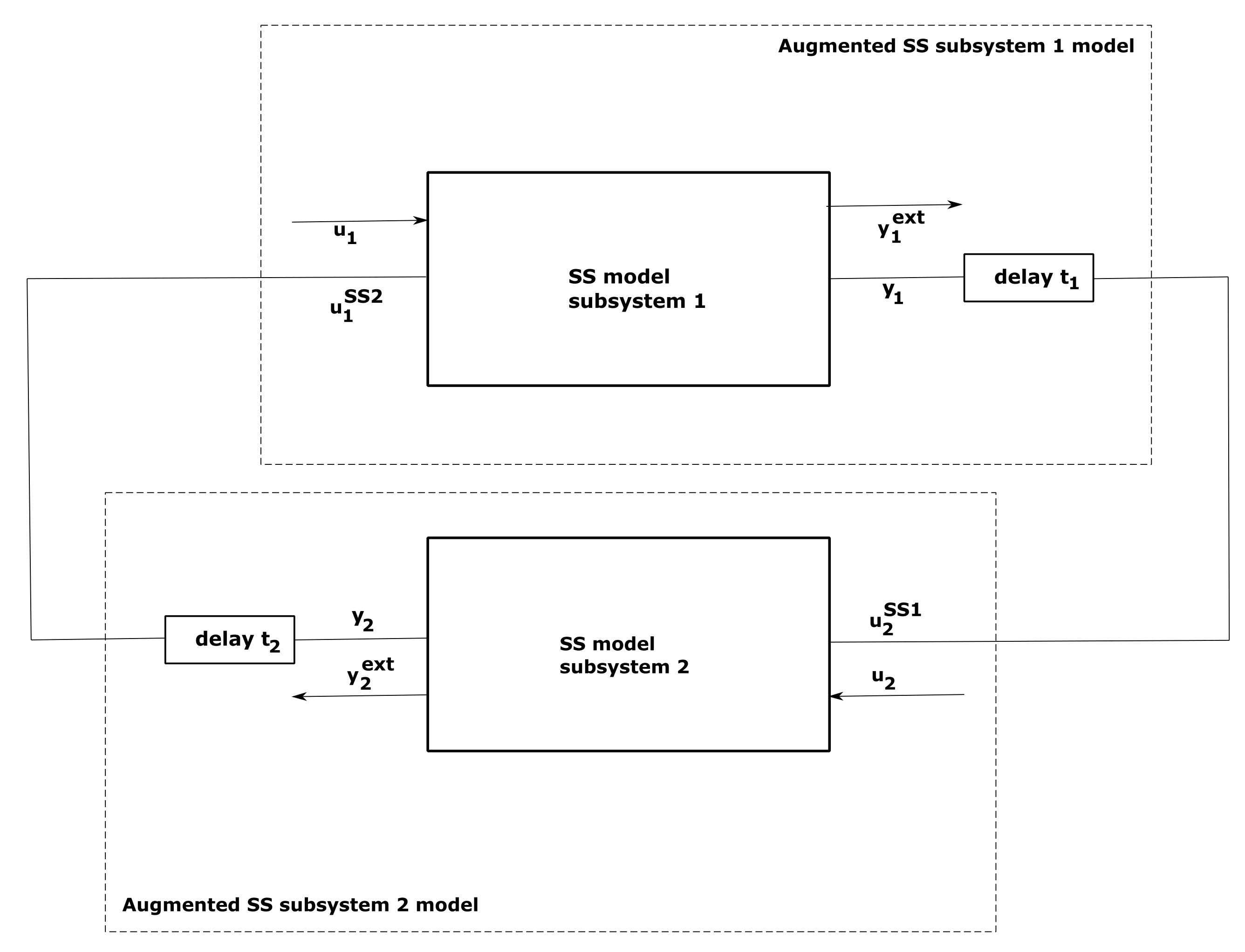
4.1. State-Space Representation of Partitioned System Model
4.2. Modal Analysis
5. Analysis and Non-Intrusive Delay-Based System Partitioning
5.1. Analysis
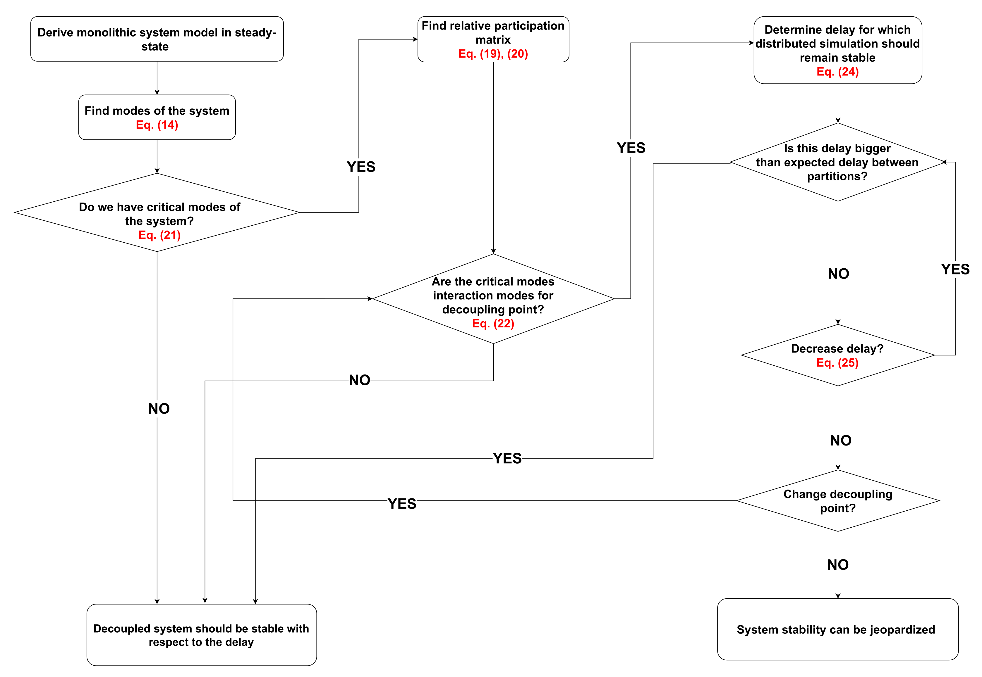
5.2. Methodology
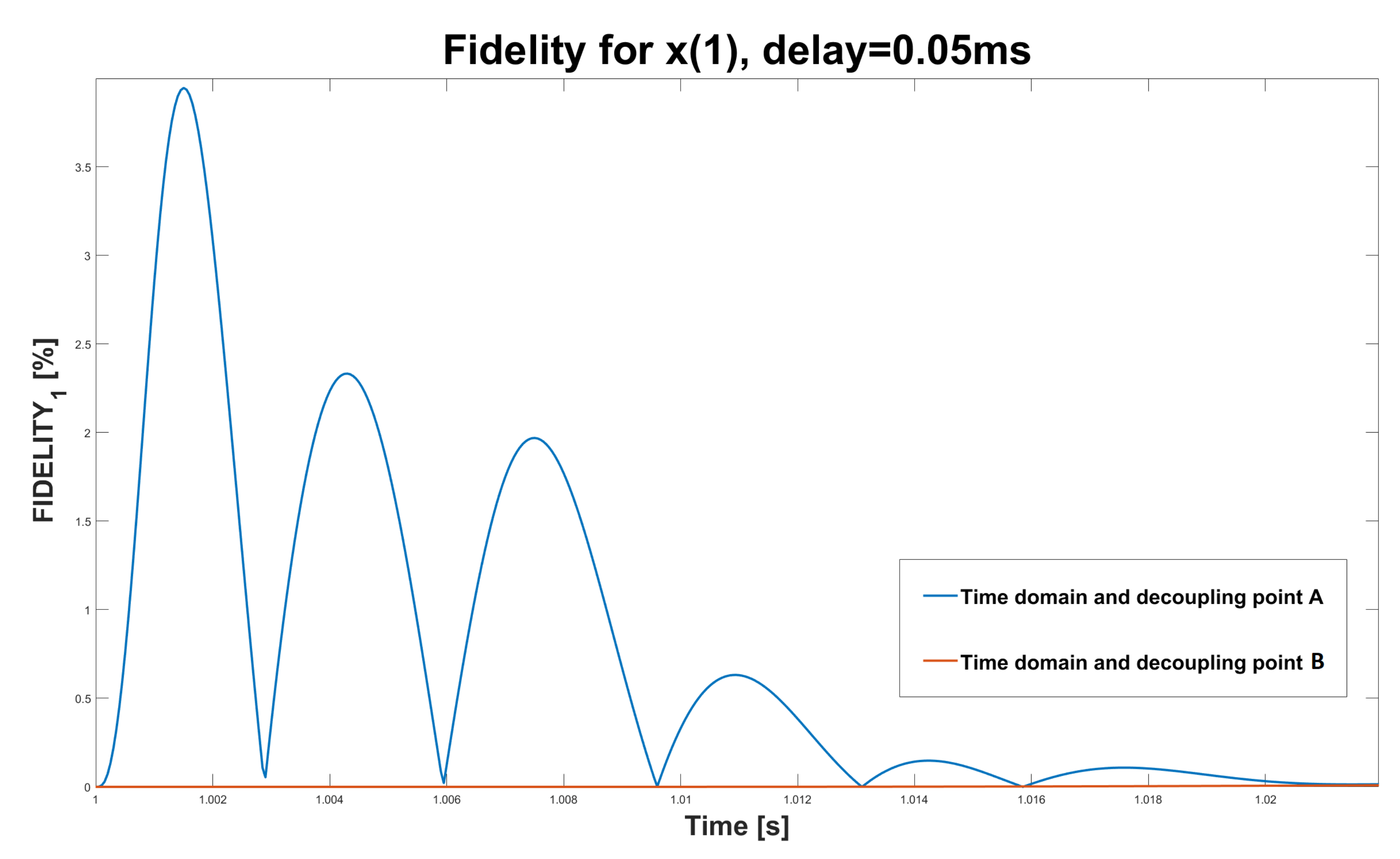
5.2.1. Method and Analysis Exemplification
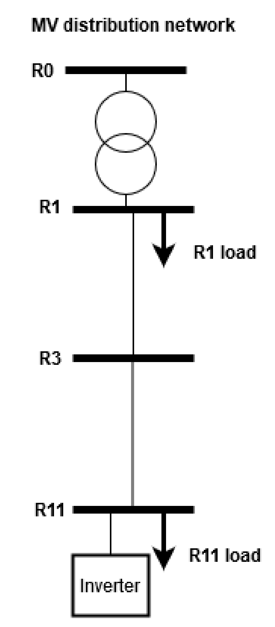
6. Testing of the Method on the Realistic Power System Model
7. Conclusions
Author Contributions
Funding
Conflicts of Interest
References
- Kotsampopoulos, P.; Lagos, D.; Hatziargyriou, N.; Faruque, M.O.; Lauss, G.; Nzimako, O.; Forsyth, P.; Steurer, M.; Ponci, F.; Monti, A.; et al. A Benchmark System for Hardware-in-the-Loop Testing of Distributed Energy Resources. IEEE Power Energy Technol. Syst. J. 2018, 5, 94–103. [Google Scholar] [CrossRef]
- Guillaud, X.; Faruque, M.O.; Teninge, A.; Hariri, A.H.; Vanfretti, L.; Paolone, M.; Dinavahi, V.; Mitra, P.; Lauss, G.; Dufour, C.; et al. Applications of Real-Time Simulation Technologies in Power and Energy Systems. IEEE Power Energy Technol. Syst. J. 2015, 2, 103–115. [Google Scholar] [CrossRef] [Green Version]
- Benigni, A.; Monti, A.; Dougal, R.A. Latency-Based Approach to the Simulation of Large Power Electronics Systems. IEEE Trans. Power Electron. 2014, 29, 3201–3213. [Google Scholar] [CrossRef]
- Bélanger, J.; Venne, P.; Paquin, J.-N. The What, Where and Why of Real-Time Simulation. Available online: https://blob.opal-rt.com/medias (accessed on 12 January 2022).
- Dufour, C.; Mahseredjian, J.; Belanger, J. A Combined State-Space Nodal Method for the Simulation of Power System Transients. IEEE Trans. Power Deliv. 2011, 26, 928–935. [Google Scholar] [CrossRef]
- Martinez-Velasco, J.A. Transient Analysis of Power Systems: Solution Techniques, Tools and Applications. 2019. Available online: https://www.wiley.com/en-us/Transient+Analysis+of+Power+Systems%3A+Solution+Techniques%2C+Tools+and+Applications-p-9781118352342 (accessed on 12 January 2022).
- Hollman, J.A.; Marti, J.R. Step-by-step eigenvalue analysis with EMTP discrete-time solutions. IEEE Trans. Power Syst. 2010, 25, 1220–1231. [Google Scholar] [CrossRef] [Green Version]
- Watson, N.; Arrillaga, J. Power Systems Electromagnetic Transients Simulation; Institution of Engineering and Technology: Stevenage, UK, 2019; pp. 193–198. [Google Scholar]
- Dommel, H.W. Digital Computer Solution of Electromagnetic Transients in Single-and Multiphase Networks. IEEE Trans. Power Appar. Syst. 1969, 88, 388–399. [Google Scholar] [CrossRef]
- Dyck, M.; Nzimako, O. Real-time simulation of large distribution networks with distributed energy resources. CIRED Open Access Proc. J. 2017, 2017, 1402–1405. [Google Scholar] [CrossRef] [Green Version]
- Brameller, A.; John, M.N.; Scott, M.R. Practical Diakoptics for Electrical Networks; Brameller, A., John, M.N., Scott, M.R., Eds.; Chapman & Hall: London, UK, 1969; 242p. [Google Scholar]
- Kron, G. Diakoptics: The Piecewise Solution of Large-Scale Systems; Madconald Technical Books; Macdonals: London, UK, 1963. [Google Scholar]
- Zhang, P.; Marti, J.; Dommel, H. Network partitioning for real-time power system simulation. In Proceedings of the 2005 International Conference on Power System Transients, Montreal, QC, Canada, 19–23 June 2005; pp. 1–6. [Google Scholar]
- Karypis, G.; Kumar, V. Multilevel Algorithms for Multi-Constraint Graph Partitioning. In Proceedings of the 1998 ACM/IEEE Conference on Supercomputing, San Jose, CA, USA, 7–13 November 1998; p. 28. [Google Scholar] [CrossRef]
- Moreira, F.A.; Martí, J.R. Latency suitability for the time-domain simulation of electromagnetic transients through network eigenanalysis. In Proceedings of the International Conference on Power Systems Transients (IPST), New Orleans, LA, USA, 28 September–2 October 2003. [Google Scholar]
- Tzounas, G.; Milano, F. Delay-based Decoupling of Power System Models for Transient Stability Analysis. IEEE Trans. Power Syst. 2020. [Google Scholar] [CrossRef]
- Uriarte, F.M. Multicore Simulation of Power System Transients; IET Power and Energy Series; The Institution of Engineering and Technology: London, UK, 2013; Volume 67. [Google Scholar]
- Ersal, T.; Gillespie, R.B.; Brudnak, M.; Stein, J.L.; Fathy, H.K. Effect of coupling point selection on distortion in Internet-distributed hardware-in-the-loop simulation. In Proceedings of the 2011 American Control Conference, San Francisco, CA, USA, 29 June–1 July 2011; pp. 3096–3103. [Google Scholar] [CrossRef]
- Ren, W.; Steurer, M.; Baldwin, T.L. Improve the Stability and the Accuracy of Power Hardware-in-the-Loop Simulation by Selecting Appropriate Interface Algorithms. IEEE Trans. Ind. Appl. 2008, 44, 1286–1294. [Google Scholar] [CrossRef]
- Abourida, S.; Bélanger, J.; Jalili-Marandi, V. Real-Time Power System Simulation: EMT vs. Phasor. In OPAL-RT Technologies: White Paper: opWP150620-sa-revA; OPAL-RT Technologies Inc.: Montreal, QC, Canada, 2016. [Google Scholar]
- Dussaud, F. An Application of Modal Analysis in Electric Power Systems to Study Inter-Area Oscillations; KTH: Stockholm, Sweden, 2015. [Google Scholar]
- Susuki, Y.; Chakrabortty, A. Introduction to Koopman Mode Decomposition for Data-Based Technology of Power System Nonlinear Dynamics. IFAC-PapersOnLine 2018, 51, 327–332. [Google Scholar] [CrossRef]
- Barocio, E.; Pal, B.; Thornhill, N.; Messina, A.R. A Dynamic Mode Decomposition Framework for Global Power System Oscillation Analysis. IEEE Trans. Power Syst. 2015, 30, 2902–2912. [Google Scholar] [CrossRef]
- Alassaf, A.; Fan, L. Dynamic Mode Decomposition in Various Power System Applications. In Proceedings of the 2019 North American Power Symposium (NAPS), Wichita, KS, USA, 13–15 October 2019; pp. 1–6. [Google Scholar] [CrossRef]
- Ramos, J.J.; Kutz, J.N. Dynamic Mode Decomposition and Sparse Measurements for Characterization and Monitoring of Power System Disturbances. arXiv 2019, arXiv:1906.03544. [Google Scholar]
- Chen, C.T. Linear System Theory and Design; Oxford University Press: Oxford, UK, 1998. [Google Scholar]
- Kundur, P.; Balu, N.; Lauby, M. Power System Stability and Control; McGraw-Hill: New York, NY, USA, 1994. [Google Scholar]
- Perezarriaga, I.; Verghese, G.; Schweppe, F. Selective Modal Analysis with Applications to Electric Power Systems, PART I: Heuristic Introduction. IEEE Trans. Power Appar. Syst. 1982, 101, 3117–3125. [Google Scholar] [CrossRef]
- Kunjumuhammed, L.; Pal, B.; Gupta, R.; Dyke, K. Stability Analysis of a PMSG-Based Large Offshore Wind Farm Connected to a VSC-HVDC. IEEE Trans. Energy Convers. 2017, 32, 1166–1176. [Google Scholar] [CrossRef]
- Beerten, J.; D’Arco, S.; Suul, J.A. Identification and Small-Signal Analysis of Interaction Modes in VSC MTDC Systems. IEEE Trans. Power Deliv. 2016, 31, 888–897. [Google Scholar] [CrossRef] [Green Version]
- Pöller, M.A. Discrete Time State Space Analysis of Electrical Networks. In Proceedings of the International Conference on Power Systems Transients, Rio de Janeiro, Brazil, 24–28 June 2001. [Google Scholar]
- CIGRE Task Force C6.04. Benchmark Systems for Network Integration of Renewable and Distributed Energy Resources. 2014. Available online: https://e-cigre.org/publication (accessed on 12 January 2022).
- Rocabert, J.; Luna, A.; Blaabjerg, F.; Rodríguez, P. Control of Power Converters in AC Microgrids. IEEE Trans. Power Electron. 2012, 27, 4734–4749. [Google Scholar] [CrossRef]
- Prodanovic, M.; Green, T.C. Control and filter design of three-phase inverters for high power quality grid connection. IEEE Trans. Power Electron. 2003, 18, 373–380. [Google Scholar] [CrossRef] [Green Version]
- Schiffer, J.; Zonetti, D.; Ortega, R.; Stankovic, A.; Sezi, T.; Raisch, J. A survey on modeling of microgrids—From fundamental physics to phasors and voltage sources. Automatica 2016, 74, 135–150. [Google Scholar] [CrossRef] [Green Version]
- Angioni, A. Uncertainty Modeling for Analysis and Design of Monitoring Systems for Dynamic Electrical Distribution Grids; RWTH Aachen University: Aachen, Germany, 2019. [Google Scholar] [CrossRef]


| Mode i | Value | |||
|---|---|---|---|---|
| −451.63 ± 904.73 · i | 0.44663 | 1011.2 | 0.62137 | |
| −77.33 ± 146.50 · i | 0.46683 | 165.65 | 3.7931 | |
| −140.91 | 1 | 140.91 | - | |
| −101.18 | 1 | 101.18 | - |
| Mode Value | |||
|---|---|---|---|
| Monolithic model-continuous | −451.63 + 904.73 ·i | 0.447 | 1.01 |
| Monolithic model-discrete | −451.27 + 904.51 ·i | 0.446 | 1.01 |
| Decoupled model | −426.01 + 919.75 ·i | 0.420 | 1.01 |
| −373.91 + 941.87 ·i | 0.369 | 1.01 | |
| −318.14 + 957.58 ·i | 0.315 | 1.01 | |
| −262.99 + 963.08 ·i | 0.263 | 9.98 | |
| −162.27 + 952.21 ·i | 0.168 | 9.66 | |
| 184.81 + 859.60 · i | −0.21 | 8.79 |
| Parameter | Value | Parameter | Value |
|---|---|---|---|
| 40 kHz | 8.5 kVA | ||
| 0.535 mH | 400 V | ||
| 9.3846 F |
Publisher’s Note: MDPI stays neutral with regard to jurisdictional claims in published maps and institutional affiliations. |
© 2022 by the authors. Licensee MDPI, Basel, Switzerland. This article is an open access article distributed under the terms and conditions of the Creative Commons Attribution (CC BY) license (https://creativecommons.org/licenses/by/4.0/).
Share and Cite
Bogdanovic, M.; Stevic, M.; Monti, A. Non-Intrusive Delay-Based Model Partitioning for Distributed Real-Time Simulation. Energies 2022, 15, 767. https://doi.org/10.3390/en15030767
Bogdanovic M, Stevic M, Monti A. Non-Intrusive Delay-Based Model Partitioning for Distributed Real-Time Simulation. Energies. 2022; 15(3):767. https://doi.org/10.3390/en15030767
Chicago/Turabian StyleBogdanovic, Milica, Marija Stevic, and Antonello Monti. 2022. "Non-Intrusive Delay-Based Model Partitioning for Distributed Real-Time Simulation" Energies 15, no. 3: 767. https://doi.org/10.3390/en15030767
APA StyleBogdanovic, M., Stevic, M., & Monti, A. (2022). Non-Intrusive Delay-Based Model Partitioning for Distributed Real-Time Simulation. Energies, 15(3), 767. https://doi.org/10.3390/en15030767