
Impact of Signalized Intersections on CO2 and NOx Emissions of Heavy Duty Vehicles


Abstract
1. Introduction
1.1. Fuel Consumption, CO2 and NOx Emissions
1.2. Transport Corridors
1.3. Emissions and Traffic Control
1.4. Previous Studies
2. Materials and Methods
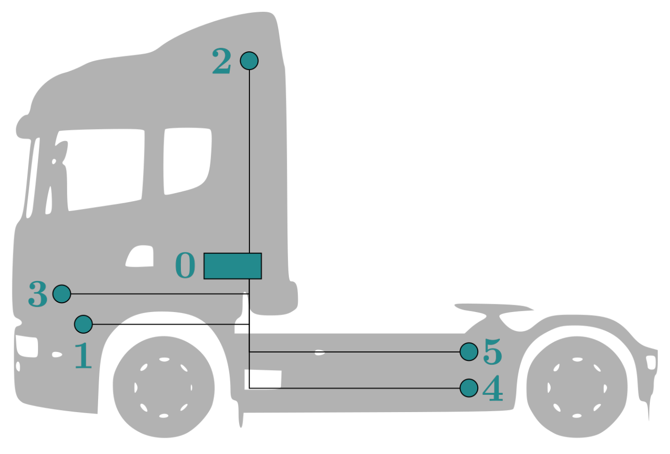
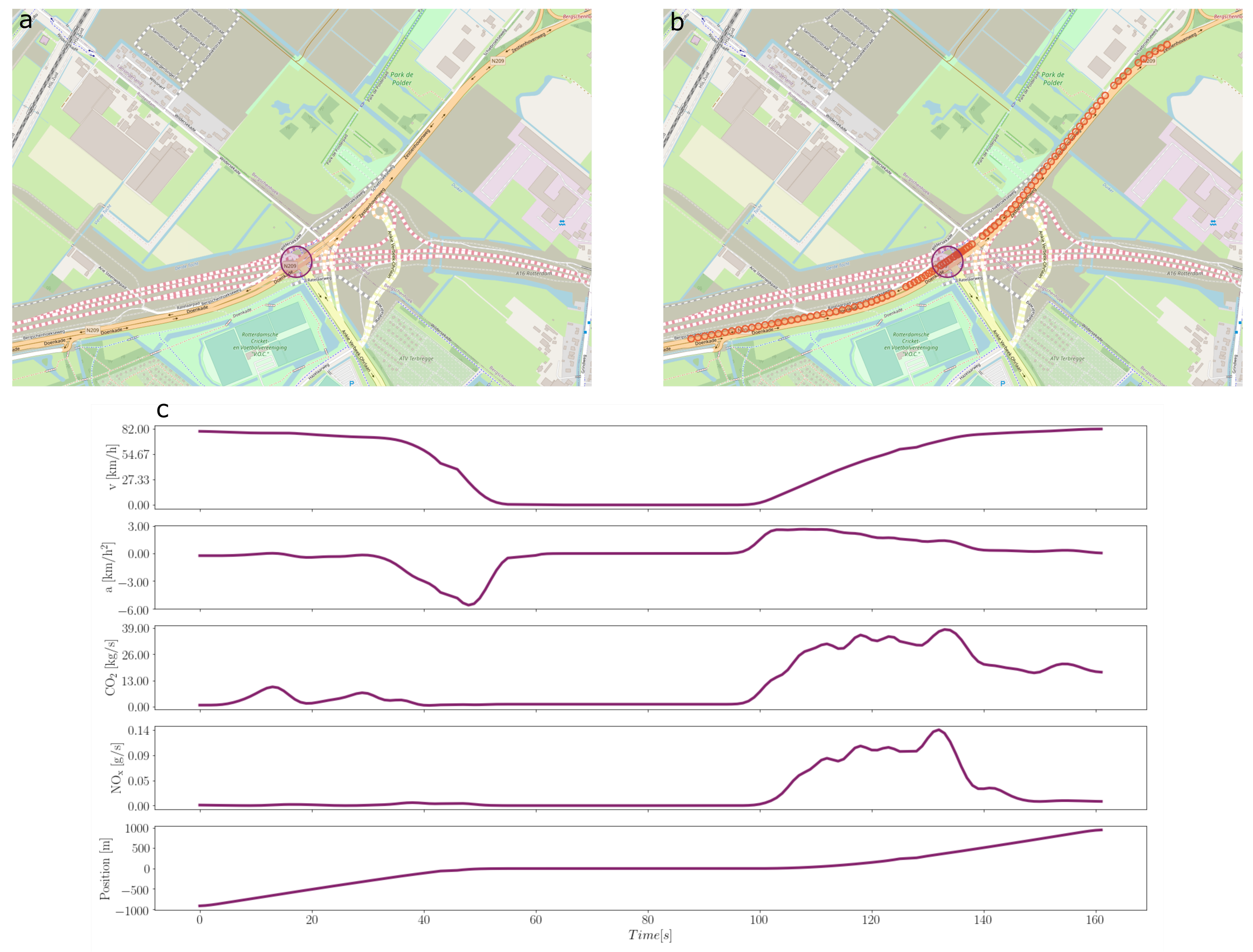
2.1. Physical Measurements and Data Acquisition
SEMS System
2.2. Data Processing
2.2.1. SEMS Preprocessing
- Calibration: Sensor data are corrected using a function based on calibration of the particular sensor in the lab;
- Speed signals from GPS and vehicles are compared and combined to produce a good and continuous signal;
- Raw cleaning: check for negative values, filter some signals for spikes, remove signals when the engine is not running, and fill small gaps in the data if possible;
- Time alignment: align signals related to emissions to signals related to the engine;
- Ammonia correction: correction of NOx concentration signal for ammonia, based on ammonia sensor values. This is necessary because the NOx sensor is cross sensitive for NH3;
- Mass flow calculation: Emissions in grams are calculated by calculating the flow of exhaust gas and multiplying it with the concentrations observed.
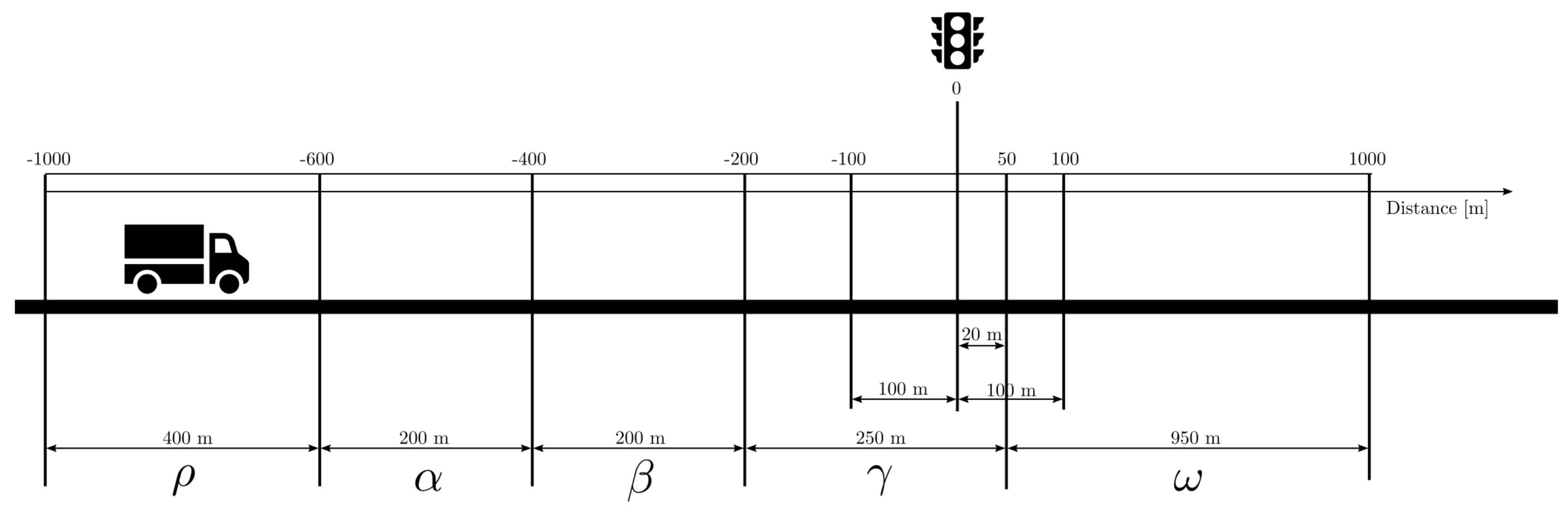
2.2.2. Data Enrichment and Selection
2.3. Analysis
2.3.1. Clustering
2.4. Outcome Measures
2.5. Impact
3. Results
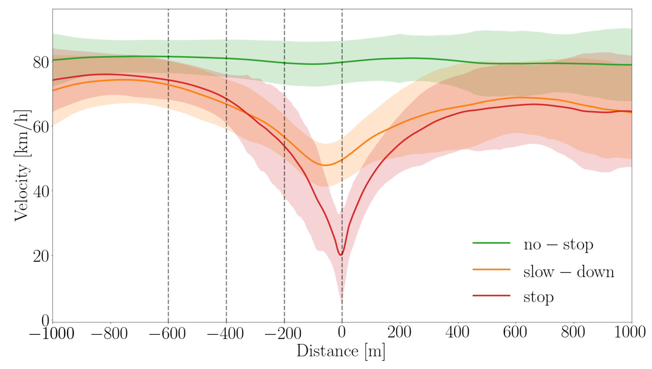
3.1. Clustering of the Speed Profiles
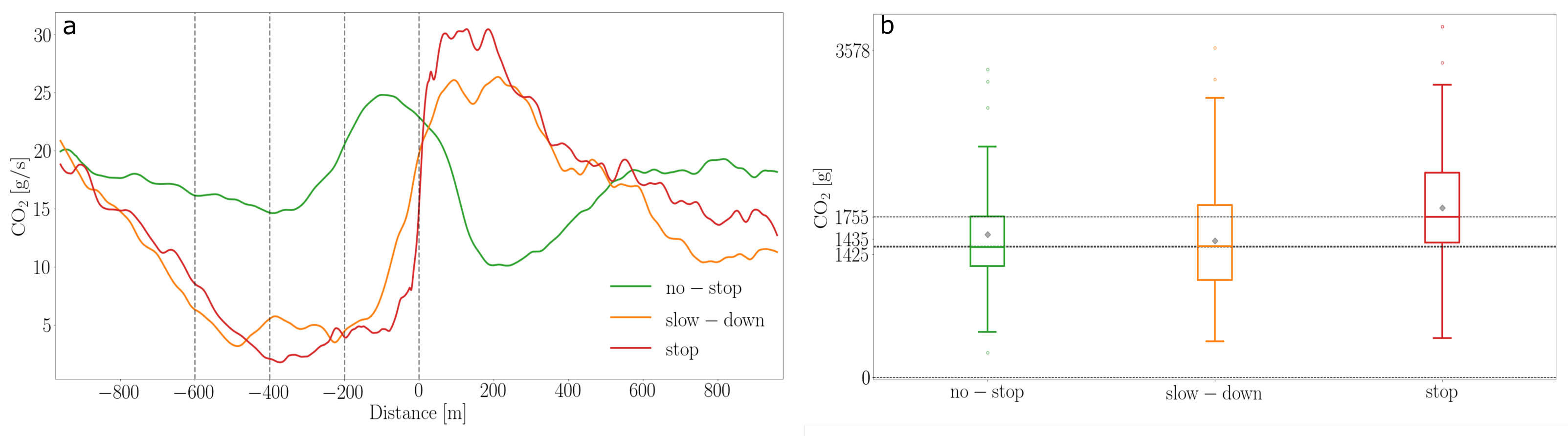
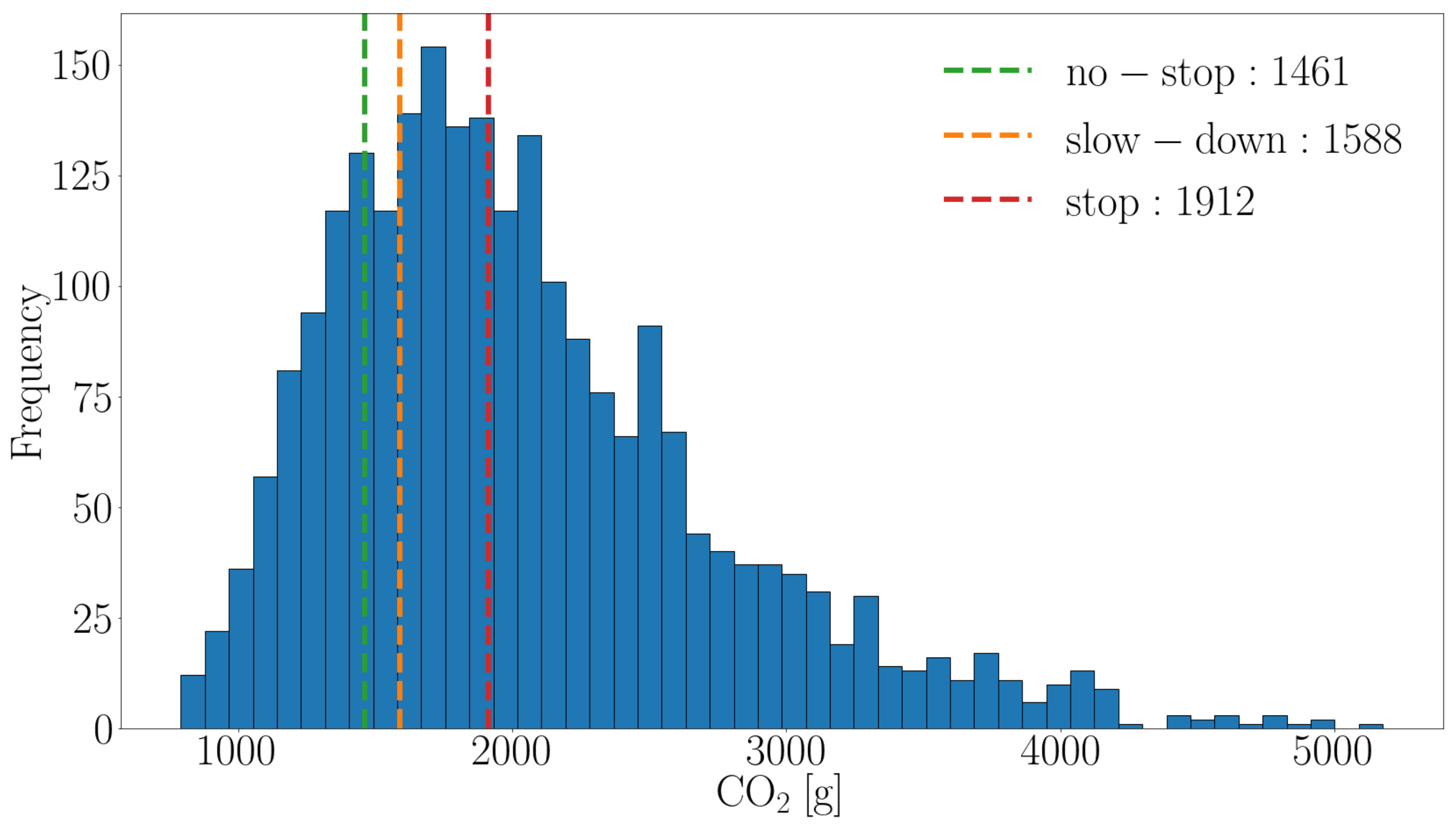
3.2. CO2 Emissions
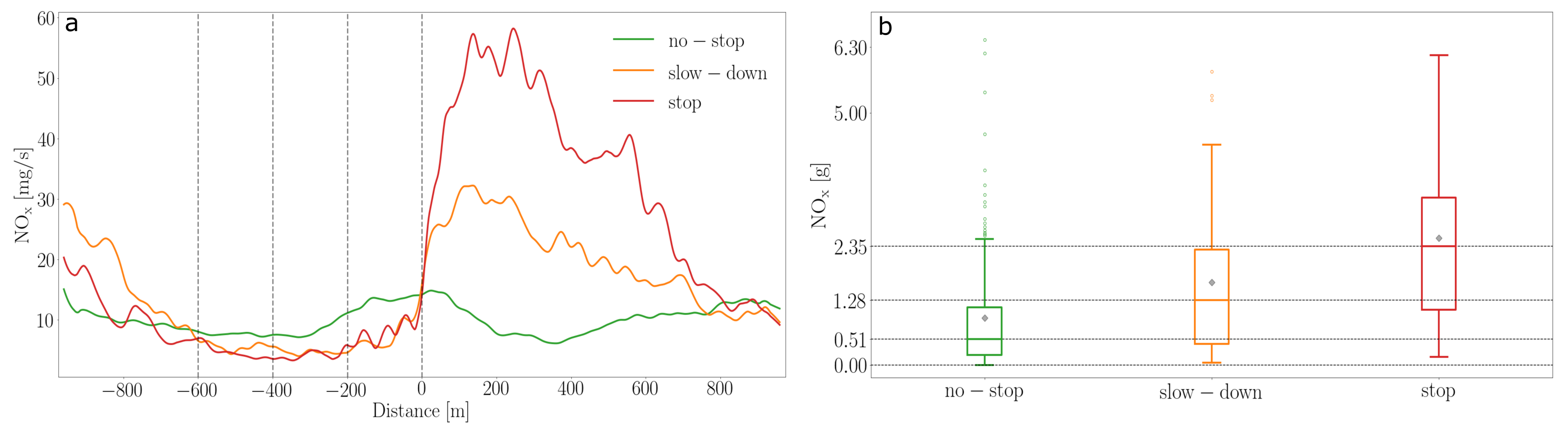
3.3. NOx Emissions
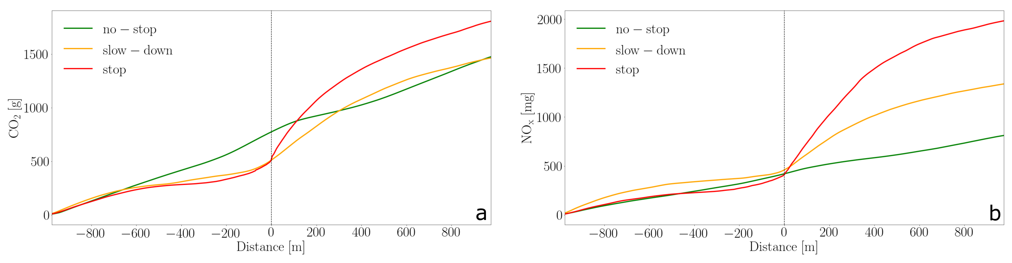
3.4. Impact
4. Discussion
5. Conclusions
Author Contributions
Funding
Institutional Review Board Statement
Informed Consent Statement
Acknowledgments
Conflicts of Interest
Abbreviations
| ITS | Intelligent Transport Systems |
| C-ITS | Cooperative Intelligent Transport Systems |
| iTLC | Intelligent Traffic Light Controller |
| HDV | Heavy-Duty Vehicles |
| GPS | Global Positioning System |
| SEMS | Smart Emissions Measurement System |
| RPM | Revolutions per minute |
| EU | European Union |
| CBS | Central Bureau for Statistics |
Appendix A
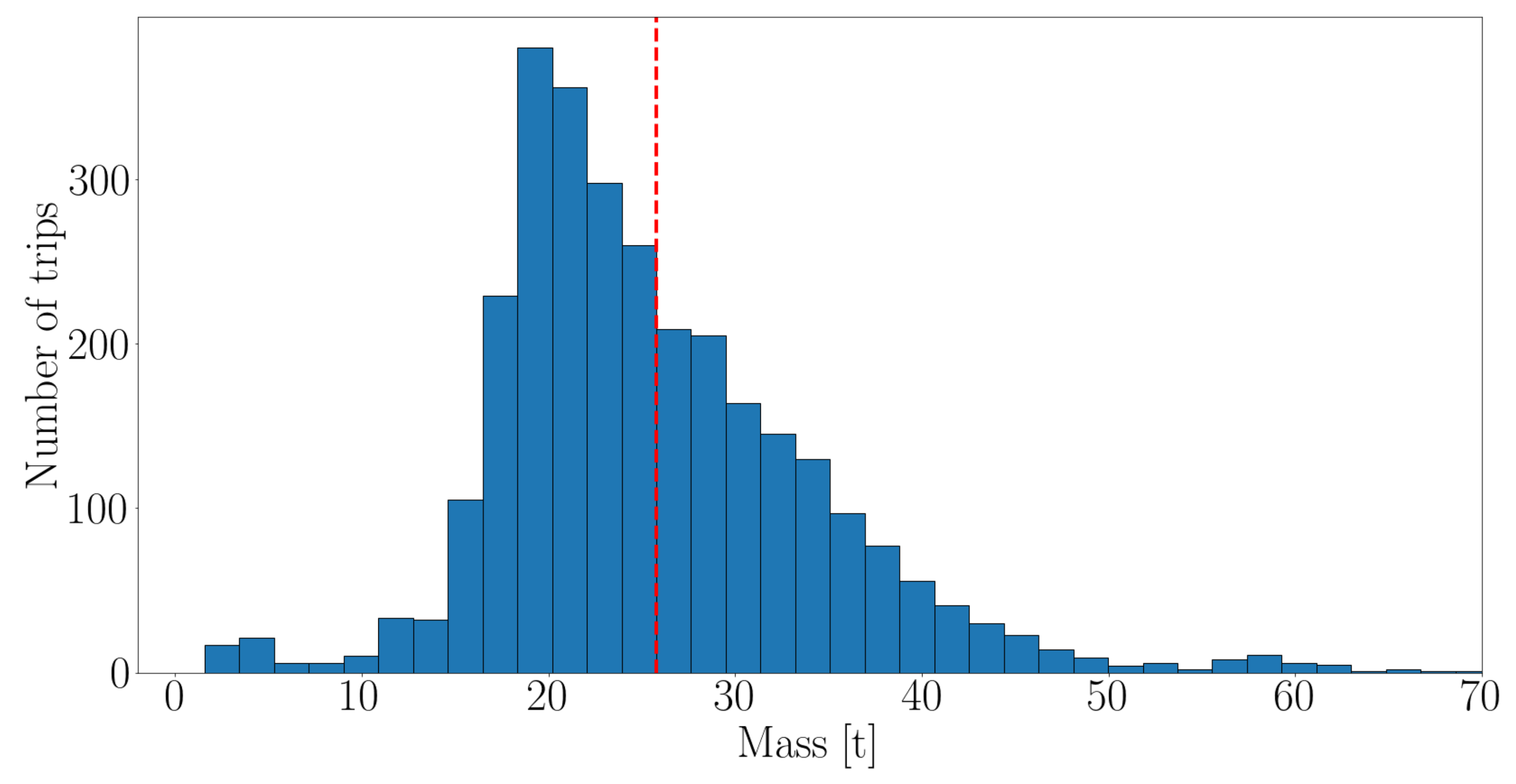
Appendix A.1. Vehicle Mass Estimation

Appendix A.2. Statistical Analysis

| Degrees of Freedom | p-Value | |
|---|---|---|
| 84.23 | 2 |
| Scenario Pair | Mean Rank Difference | p-Value |
|---|---|---|
| slow-down × no-stop | 52.64967 | 0.0037 |
| stop × no-stop | 197.80831 | |
| slow-down × stop | 145.15864 |
| Degrees of Freedom | p-Value | |
|---|---|---|
| 142.85 | 2 |
| Scenario Pair | Mean Rank Difference | p-Value |
|---|---|---|
| slow-down × no-stop | 141.68511 | |
| stop × no-stop | 203.46920 | |
| slow-down × stop | 61.78409 | 0.0019 |
References
- Mendoza-Villafuerte, P.; Suarez-Bertoa, R.; Giechaskiel, B.; Riccobono, F.; Bulgheroni, C.; Astorga, C.; Perujo, A. NOx, NH3, N2O and PN real driving emissions from a Euro VI heavy-duty vehicle. Impact of regulatory on-road test conditions on emissions. Sci. Total Environ. 2017, 609, 546–555. [Google Scholar] [CrossRef] [PubMed]
- Liu, Y.S.; Cao, Y.; Hou, J.J.; Zhang, J.T.; Yang, Y.O.; Liu, L.C. Identifying common paths of CO2 and air pollutants emissions in China. J. Clean. Prod. 2020, 256, 120599. [Google Scholar] [CrossRef]
- Abera, A.; Friberg, J.; Isaxon, C.; Jerrett, M.; Malmqvist, E.; Sjöström, C.; Taj, T.; Vargas, A.M. Air Quality in Africa: Public Health Implications. Annu. Rev. Public Health 2021, 42, 193–210. [Google Scholar] [CrossRef] [PubMed]
- Cohen, A.J.; Brauer, M.; Burnett, R.; Anderson, H.R.; Frostad, J.; Estep, K.; Balakrishnan, K.; Brunekreef, B.; Dandona, L.; Dandona, R.; et al. Estimates and 25-year trends of the global burden of disease attributable to ambient air pollution: An analysis of data from the Global Burden of Diseases Study 2015. Lancet 2017, 389, 1907–1918. [Google Scholar] [CrossRef]
- Burnett, R.; Chen, H.; Szyszkowicz, M.; Fann, N.; Hubbell, B.; Pope, C.A.; Apte, J.S.; Brauer, M.; Cohen, A.; Weichenthal, S.; et al. Global estimates of mortality associated with long-term exposure to outdoor fine particulate matter. Proc. Natl. Acad. Sci. USA 2018, 115, 9592–9597. [Google Scholar] [CrossRef]
- Harrison, R.M.; Allan, J.; Carruthers, D.; Heal, M.R.; Lewis, A.C.; Marner, B.; Murrells, T.; Williams, A. Non-exhaust vehicle emissions of particulate matter and VOC from road traffic: A review. Atmos. Environ. 2021, 262, 118592. [Google Scholar] [CrossRef]
- Ittmann, H.W.; King, D. State of Logistics—An overview of logistics in South Africa. In Proceedings of the CSIR 3rd Biennial Conference 2010, Science Real and Relevant, CSIR International Convention Centre, Pertoria, South Africa, 30 August–1 September 2010; p. 11. [Google Scholar]
- Havenga, J.; Pienaar, W. Quantifying Freight Transport Volumes in Developing Regions: Lessons Learnt from South Africa’s Experience During the 20th Century. Econ. Hist. Dev. Reg. 2012, 27, 87–113. [Google Scholar] [CrossRef]
- Kaack, L.H.; Vaishnav, P.; Morgan, M.G.; Azevedo, I.L.; Rai, S. Decarbonizing intraregional freight systems with a focus on modal shift. Environ. Res. Lett. 2018, 13, 083001. [Google Scholar] [CrossRef]
- Blauwens, G.; Vandaele, N.; de Voorde, E.V.; Vernimmen, B.; Witlox, F. Towards a Modal Shift in Freight Transport? A Business Logistics Analysis of Some Policy Measures. Transp. Rev. 2006, 26, 239–251. [Google Scholar] [CrossRef]
- Dekker, R.; Bloemhof, J.; Mallidis, I. Operations Research for green logistics – An overview of aspects, issues, contributions and challenges. Eur. J. Oper. Res. 2012, 219, 671–679. [Google Scholar] [CrossRef]
- Hwang, T.; Ouyang, Y. Freight shipment modal split and its environmental impacts: An exploratory study. J. Air Waste Manag. Assoc. 2013, 64, 2–12. [Google Scholar] [CrossRef]
- Bickford, E. Emissions and Air Quality Impacts of Freight Transportation. Ph.D. Thesis, The University of Wisconsin-Madison, Madison, WI, USA, 2012. [Google Scholar]
- Huang, Y.; Chuen Mok, W.; Shing Yam, Y.; Zhou, J.L.; Surawski, N.C.; Organ, B.; Chan, E.F.; Mofijur, M.; Mahlia, T.M.I.; Ong, H.C. Evaluating in-use vehicle emissions using air quality monitoring stations and on-road remote sensing systems. Sci. Total Environ. 2020, 740, 139868. [Google Scholar] [CrossRef]
- Ang-Olson, J.; Ostria, S. Assessing the Effects of Freight Movement on Air Quality at the National and Regional Level; Office of Natural and Human Environment, US Federal Highway Administration: Washington, DC, USA, 2005. [Google Scholar]
- Roberts, M.; Melecky, M.; Bougna, T.; Xu, Y.S. Transport corridors and their wider economic benefits: A quantitative review of the literature. J. Reg. Sci. 2019, 60, 207–248. [Google Scholar] [CrossRef]
- Van Weenen, R.L.; Burgess, A.; Francke, J. Study on the Implementation of the TEN-T Regulation–The Netherlands Case. Transp. Res. Procedia 2016, 14, 484–493. [Google Scholar] [CrossRef][Green Version]
- The European Parliament and the council of the European Union. On Union Guidelines for the Development of the Trans- European Transport Network and Repealing Decision. Regulation (EU) No 1315/2013 Official Journal of the European Union L 348, 20.12.2013. 2013. pp. 1–128. Available online: http://data.europa.eu/eli/reg/2013/1315/oj (accessed on 6 December 2021). [CrossRef]
- Commission of the European Communities. Green Paper: TEN-T: A Policy Review. Towards a Better Integrated Transeuropean Network at the Service of the Common Transport Policy. 2009. Available online: https://eur-lex.europa.eu/legal-content/en/TXT/?uri=CELEX%3A52009DC0044 (accessed on 6 December 2021).
- Öberg, M.; Nilsson, K.L.; Johansson, C. Major transport corridors: The concept of sustainability in EU documents. Transp. Res. Procedia 2017, 25, 3694–3702. [Google Scholar] [CrossRef]
- Conference of Europeans Directors of Roads. Trans-European Road Network Performance Report; Conference of Europeans Directors of Roads: Brussels, Belgium, 2017. [Google Scholar]
- Ministry of Instrastructure and Watermanagement. MIRT-overview, Meerjarenprogramma Infrastructuur, Ruimte en Transport (MIRT); Ministry of Instrastructure and Watermanagement: Hague, The Netherlands, 2020. [Google Scholar]
- Peters, J.; McCourt, R.; Hurtado, R. Reducing carbon emissions and congestion by coordinating traffic signals. Inst. Transp. Eng. ITE J. 2009, 79, 25. [Google Scholar]
- Barth, M.; Boriboonsomsin, K. Real-World Carbon Dioxide Impacts of Traffic Congestion. Transp. Res. Rec. J. Transp. Res. Board 2008, 2058, 163–171. [Google Scholar] [CrossRef]
- Tully, I.M.S.N.Z. Synthesis of Sequences for Traffic Signal Controllers Using Techniques of the Theory of Graphs; OUEL Report; University of Oxford, Department of Engineering Science, Engineering Laboratory: Oxford, UK, 1976. [Google Scholar]
- Guberinic, S.; Senborn, G.; Lazic, B. Optimal Traffic Control: Urban Intersections; CRC Press: Boca Raton, FL, USA, 2008. [Google Scholar]
- Klein, L.A.; Mills, M.K.; Gibson, D.R. Traffic Detector Handbook; US Department of Transportation, Federal Highway Administration, Research, Development, and Technology, Turner-Fairbank Highway Research Center: Washington, DC, USA, 2006. [Google Scholar]
- Robertson, D.; Bretherton, R. Optimizing networks of traffic signals in real time-the SCOOT method. IEEE Trans. Veh. Technol. 1991, 40, 11–15. [Google Scholar] [CrossRef]
- Sims, A.; Dobinson, K. The Sydney coordinated adaptive traffic (SCAT) system philosophy and benefits. IEEE Trans. Veh. Technol. 1980, 29, 130–137. [Google Scholar] [CrossRef]
- Middleham, F. VETAG-TEST; Technical Report; Verkeersbureau Amsterdam: Amsterdam, The Netherlands, 1976. [Google Scholar]
- Meyer, F. Points and Traffic Lights Under Common Control Using Vetag. Railw. Gaz. Int. 1975, 131, 193–194. [Google Scholar]
- Ros, W. VECOM: A powerful local communication channel between vehicle-borne and roadside systems. In Proceedings of the ESA Workshop on Land Mobile Services by Satellite, Noordwijk, The Netherlands, 3–4 June 1986; pp. 23–25. [Google Scholar]
- Festag, A. Cooperative intelligent transport systems standards in europe. IEEE Commun. Mag. 2014, 52, 166–172. [Google Scholar] [CrossRef]
- Roess, R. Traffic Engineering; Pearson: Upper Saddle River, NJ, USA, 2011. [Google Scholar]
- Chang, D.J.; Morlok, E.K. Vehicle Speed Profiles to Minimize Work and Fuel Consumption. J. Transp. Eng. 2005, 131, 173–182. [Google Scholar] [CrossRef]
- Wang, J.; Rakha, H.A. Fuel consumption model for heavy duty diesel trucks: Model development and testing. Transp. Res. Part Transp. Environ. 2017, 55, 127–141. [Google Scholar] [CrossRef]
- Guardiola, C.; Pla, B.; Pandey, V.; Burke, R. On the potential of traffic light information availability for reducing fuel consumption and NOx emissions of a diesel light-duty vehicle. Proc. Inst. Mech. Eng. Part D J. Automob. Eng. 2019, 234, 981–991. [Google Scholar] [CrossRef]
- Meneguzzer, C.; Gastaldi, M.; Rossi, R.; Gecchele, G.; Prati, M.V. Comparison of exhaust emissions at intersections under traffic signal versus roundabout control using an instrumented vehicle. Transp. Res. Procedia 2017, 25, 1597–1609. [Google Scholar] [CrossRef]
- Koenders, E. FREILOT. Urban Freight Energy Efficiency Pilot. D. FL. 3.1 Final Operation Report. 2012. Available online: https://cordis.europa.eu/docs/projects/cnect/0/238930/080/deliverables/001-DFL31Finaloperationreportv10.pdf (accessed on 6 December 2021).
- Mitsakis, E.; Salanova Grau, J.M.; Aifandopoulou, G.; Tona, P.; Vreeswijk, J.; Somma, G.; Blanco, R.; Alcaraz, G.; Jeftic, Z.; Toni, A.; et al. Large scale deployment of cooperative mobility systems in Europe: COMPASS4D. In Proceedings of the 2014 International Conference on Connected Vehicles and Expo (ICCVE), Vienna, Austria, 3–7 November 2014; pp. 469–476. [Google Scholar] [CrossRef]
- Vreeswijk, J.; Vernet, G.; Huebner, Y.; Jeftic, Z.; Tona, P.; Martinez, J.M.; Mitsakis, E.; Alcaraz, G. Compass4d: Cooperative mobility pilot on safety and sustainability services for deployment. In Proceedings of the 10th ITS European Congress, Helsinki, Finland, 16–19 June 2014. [Google Scholar]
- Agarwal, A.K.; Mustafi, N.N. Real-world automotive emissions: Monitoring methodologies, and control measures. Renew. Sustain. Energy Rev. 2021, 137, 110624. [Google Scholar] [CrossRef]
- Van Kempen, E.; de Ruiter, J.; Souman, J.; van Ark, E.J.; Deschle, N.; Oudenes, L.; Geurts, M.; van der Horst, R.; Janssen, R.; Dinalog, T. Real-World Impacts of Truck Driving with Adaptive Cruise Control on Fuel Consumption, Driver Behaviour and Logistics; Report Number 10516; TNO Publications, The Hague, The Netherlands 2021. Available online: https://repository.tudelft.nl/islandora/object/uuid%3A7bd21500-957a-492d-ad42-4d3c22d55a37 (accessed on 6 December 2021).
- Kadijk, G.; Ligterink, N.; Spreen, J. On-Road NOx and CO2 Investigations of Euro 5 Light Commercial Vehicles 2015. Report Number 10192; TNO Publications: The Hague, The Netherlands. Available online: https://repository.tno.nl//islandora/object/uuid:d212320e-7b4c-4440-ae93-3dfe386c9dec (accessed on 6 December 2021).
- Vermeulen, R.J.; Ligterink, N.E.; Vonk, W.A.; Baarbé, H.L. A Smart and Robust NOx Emission Evaluation Tool for the Environmental Screening of Heavy-Duty Vehicles. In Proceedings of the 19th International Transport and Air Pollution Conference 2012, Thessaloniki, Greece, 26–27 November 2012; pp. 1–11. [Google Scholar]
- Kadijk, G.; Vermeulen, R.; Buskermolen, E.; Elstgeest, M.; van Heesen, D.; Heijne, V.; Ligterink, N.; van der Mark, P. NO_x Emissions of Eighteen Diesel Light Commercial Vehicles: Results of the Dutch Light-Duty Road Vehicle Emission Testing Programme 2017; TNO: Delft, The Netherlands, 2017; p. R11473. [Google Scholar]
- Heepen, F.; Yu, W. SEMS for Individual Trip Reports and Long-Time Measurement; SAE Technical Paper Series; SAE International: Warrendale, PA, USA, 2019. [Google Scholar] [CrossRef]
- Luxen, D.; Vetter, C. Real-time routing with OpenStreetMap data. In Proceedings of the 19th ACM SIGSPATIAL International Conference on Advances in Geographic Information Systems (GIS ’11), Chicago, IL, USA, 1–4 November 2011; ACM: New York, NY, USA, 2011; pp. 513–516. [Google Scholar] [CrossRef]
- OpenStreetMap Contributors. Planet Dump Retrieved from. 2020. Available online: https://www.openstreetmap.org; https://planet.osm.org (accessed on 6 December 2021).
- Maurya, A.K.; Bokare, P.S. Study of Deceleration Behaviour of Different Vehicle Types. Int. J. Traffic Transp. Eng. 2012, 2, 253–270. [Google Scholar] [CrossRef]
- Ligterink, N.E. On-Board Determination of Average Dutch Driving Behaviour for Vehicle Emissions; TNO: Utrecht, The Netherlands, 2016; p. R10188. [Google Scholar]
- Centraal Bureau voor de Statistiek. Available online: https://www.cbs.nl/ (accessed on 6 December 2021).
- Council of European Union. Council Regulation (EU) No 595/2009. 2009. Available online: https://eur-lex.europa.eu/legal-content/EN/TXT/?uri=CELEX:02009R0595-20200901 (accessed on 6 December 2021).
- Council of European Union. Council regulation (EU) No 582/2011. 2011. Available online: https://eur-lex.europa.eu/legal-content/EN/TXT/?uri=CELEX:02011R0582-20180722 (accessed on 6 December 2021).
- Eurostat. Summary Of Annual Road Freight Transport By Type Of Operation And Type Of Transport. 2012. Available online: https://ec.europa.eu/eurostat/databrowser/product/view/ROAD_GO_TA_TOTT (accessed on 6 December 2021).
- Clark, N.N.; Kern, J.M.; Atkinson, C.M.; Nine, R.D. Factors Affecting Heavy-Duty Diesel Vehicle Emissions. J. Air Waste Manag. Assoc. 2002, 52, 84–94. [Google Scholar] [CrossRef]
- Kruskal, W.H.; Wallis, W.A. Use of ranks in one-criterion variance analysis. J. Am. Stat. Assoc. 1952, 47, 583–621. [Google Scholar] [CrossRef]
- Dunn, O.J. Multiple comparisons among means. J. Am. Stat. Assoc. 1961, 56, 52–64. [Google Scholar] [CrossRef]
- R Core Team. R: A Language and Environment for Statistical Computing; R Foundation for Statistical Computing: Vienna, Austria, 2017. [Google Scholar]


| Engine | Power [kW] |
|---|---|
| XF 440 FTG | 320 |
| XF 460 FTG | 341 |
| XF 440 FT | 324 |
| XF 480 FTG | 353 |
| XF 480 MX-13 | 355 |
| Cluster | Number of Passages |
|---|---|
| no-stop | 378 |
| slow-down | 349 |
| stop | 175 |
| CO2 [g] | |
| HDV yearly total CO2 [g] | |
| Potential fraction saved [%] |
Publisher’s Note: MDPI stays neutral with regard to jurisdictional claims in published maps and institutional affiliations. |
© 2022 by the authors. Licensee MDPI, Basel, Switzerland. This article is an open access article distributed under the terms and conditions of the Creative Commons Attribution (CC BY) license (https://creativecommons.org/licenses/by/4.0/).
Share and Cite
Deschle, N.; van Ark, E.J.; van Gijlswijk, R.; Janssen, R. Impact of Signalized Intersections on CO2 and NOx Emissions of Heavy Duty Vehicles. Energies 2022, 15, 1242. https://doi.org/10.3390/en15031242
Deschle N, van Ark EJ, van Gijlswijk R, Janssen R. Impact of Signalized Intersections on CO2 and NOx Emissions of Heavy Duty Vehicles. Energies. 2022; 15(3):1242. https://doi.org/10.3390/en15031242
Chicago/Turabian StyleDeschle, Nicolás, Ernst Jan van Ark, René van Gijlswijk, and Robbert Janssen. 2022. "Impact of Signalized Intersections on CO2 and NOx Emissions of Heavy Duty Vehicles" Energies 15, no. 3: 1242. https://doi.org/10.3390/en15031242
APA StyleDeschle, N., van Ark, E. J., van Gijlswijk, R., & Janssen, R. (2022). Impact of Signalized Intersections on CO2 and NOx Emissions of Heavy Duty Vehicles. Energies, 15(3), 1242. https://doi.org/10.3390/en15031242