1. Introduction
Simulation and optimization are vital components of science and economics. Models serve the purpose of digitally simulating real systems and subsequently investigating the behavior and sensitivity of different scenarios and design choices of “what-if-analysis” by changing input parameters for the models. The energy system relies heavily on simulation and optimization. They are used to adequately dimension grid systems, to coordinate supply and demand, to optimize welfare for the marketing of energy and flexibility, and to predict the behavior of the grid system in future scenarios.
Such simulation models are knowledge-driven and hence require a profound understanding of input data and its functional relationship to the desired output. In many cases the functional relationships are very complex and involve optimization problems or the solution of complex (partial differential) equations. The simulation time often becomes a challenge with increasing levels of detail and knowledge, larger numbers of scenarios, or additional systems to be simulated. The runtime of these models can be improved with better (e.g., cloud-based) scaling, optimization of the model, or simplification (e.g., of the input data or functional relationship). While scaling comes with additional costs and simplification decreases the models’ accuracy, optimization can include the use of machine learning (ML (a list of abbreviations used in this paper can be found in Abbreviations)).
In contrast to knowledge-based models, supervised machine learning algorithms do not necessarily require prior knowledge of the functional relationship. Instead, they need sufficient amounts of data to “learn” the functional relationship of input and output. While the training process is often time consuming, their application is quicker and computationally less expensive. In some cases, predictions of trained ML models, e.g., for fluid dynamics, can be conducted in almost real-time, while simulation models employing the Navier–Stokes equation are computationally complex and much slower.
A current field of science deals with the combination of knowledge-based simulations and data-based ML. This field is often called emulation, surrogate-modeling, or meta-modeling. The goal is to substitute (parts of) a model with ML to speed it up. In Section 0, we shed light on the current state of research, show examples of how much faster classical simulation models can be made using this approach, and highlight our contributions in this field. The methodology of this paper is described in Section 0. A challenge of this approach is the limitation of available data for training and testing. Due to their high computational and time complexity, simulation models often cannot be used to generate abundant training data. Sampling methods to determine the best training data, even for small sample sizes, are compared, and different approaches for energy-economic use cases are introduced in Section 0. This paper introduces the combination of ML-based emulation and time series aggregation. In Section 0, time series aggregation is described, applied, and evaluated on energy economic data. These principles and results are then applied in Section 0. The emulation of simulation models with ML models and time series aggregation is shown and evaluated on an energy-economic case study in the context of pricing mechanisms in peer-to-peer (P2P) energy communities. The goal of this section is to use both TSA and emulation, show their impact on model accuracy and performance, and evaluate the synergy of these methods. In Section 0.5, we show energy-economic results of the pricing methods in approximately 12,000 German municipalities. The method, as well as the paper’s results, are discussed in Section 0, and a summary and outlook are given in Section 0.
2. Literature Review
Many engineering tasks in the energy sector require simulations. Often these simulations must be repeated many times, e.g., for a large population, different scenarios, sensitivity analysis, uncertainty quantification, or multiple design choices. The time-consuming nature of individual simulations combined with the necessary repetitions make such simulations a limiting factor in projects. An option to decrease simulation time is the use of supervised ML models. Once trained, they are capable of significantly decreasing simulation times, but often at the cost of accuracy. In the following subsections we introduce the current state of the literature, define relevant terms, give insight into practical applications, and show the importance of sampling methods in this field.
2.1. Introduction of Emulation, Surrogate, and Meta-Models
ML models can be used instead of a knowledge-based simulation model to mimic its behavior entirely, or to substitute parts of the simulation to reduce time-consuming bottlenecks within the simulation framework. The process of substituting a simulation model by ML is called emulation, meta- or surrogate modeling. In current scientific works, the terms “emulator”, “meta-model” or “surrogate model” are often used interchangeably [
1].
In [
2], Köhnen et al. further define “hybrid meta models” as meta-models that are trained based on a simulation or optimization model, rather than on real data.
McGregor in [
3] refers to an emulator as a model where “some functional part of the model is carried out by a part of the real system”. The authors also consider the definition valid when reversed: “an emulation-model is one where a part of the real system is replaced by a model.” In the case of this work, the “real system” is a model itself. In this context, “emulation” (lat. aemulator) is considered the reproduction of the behavior of a simulation model as close as possible to the original, while still retaining parts of the simulation model.
Meta-models (“a model of models”) or surrogate models substitute the entire simulation model, e.g., by ML-based regression or classical polynomial functions [
2]. The schematic difference of simulation, emulation, and surrogate/meta-models is shown in
Figure 1.
An advantage of emulation over surrogate- or meta-models is the reduced functional relationship, because only a fraction of the complexity is covered by an ML algorithm. Additionally, the results are easier to interpret, since many parts of the original model components, and hence the knowledge about the functional relationship, are retained. The combination of white- (simulation) and black-box models (ML) can improve the transparency of ML models [
2]. This combination of simulation and emulation reduces the necessary data for training and allows the use of simpler and more robust ML models (e.g., random forest or linear regression). If, however, not a single model component but many of the model components slow down the simulation process, surrogate or meta-models are more advantageous, since they substitute the entire simulation model. Terms are used interchangeably for the literature review in this section. In Section 0, we define our own model as a hybrid emulator based on this distinction, since parts of the simulation framework are retained.
In this paper, emulation is performed with regression. Regression, similar to classification, is a technique of supervised ML. One advantage of these models is to be able to perform calculations many times faster than classical, knowledge-based simulation models [
4]. To determine the functional relationships between predictor variables (input,
) and one or more corresponding dependent variables (output,
), ML models are applied to sufficient amounts of data [
5]. The functional relationship
can be approximated with a regression model
[
5], with ε being the error between a predicted label
and a true (known) label
y [
6].
Jiang et al. give a detailed introduction to surrogate-models as well as multiple sampling methods [
7]. The authors introduce multiple types of models (e.g., classical, ensemble, and multi-fidelity surrogate-models). While classical surrogate-models include, for example, a single ML model, such as an artificial neural network, an ensemble of surrogate-models “is a surrogate-model composed of a series of surrogate-models combined through a weighted sum”. This increases the robustness of the prediction. The idea of multi-fidelity surrogate models is the combination of high-fidelity (HF) simulation models with high accuracy but high computational complexity with low-fidelity (LF) models with low computational cost but low accuracy.
In the following, we give a comprehensive overview of the current scientific state and applications of machine-learning-based emulation, meta-, and surrogate models. We present the current scientific works as well as the current works about ML with small datasets and the importance of sampling methods.
2.2. Modeling Process
In the literature (e.g., see [
7,
8,
9,
10,
11]), the process of developing a surrogate-model generally includes the steps shown in
Figure 2.
Figure 2 depicts the workflow for surrogate-modeling as found in current scientific literature. The input parameters depend on the simulation framework [
12]. The input values of the simulation model are referred to as “input parameters”, whereas the input values of the machine learning models are referred to as “input features”. Hyperparameters are additional presets that control the learning process of a machine learning model and are set prior to the learning process itself. In most cases (e.g., for partial differential equations), the input parameters are continuous, often uniformly distributed and without known boundaries. Sampling methods are applied to these input parameters and then used in the simulation framework. The results are utilized for training and evaluation of the ML models. The models’ hyperparameters are optimized, using e.g., a grid search [
13]. Depending on the sampling method (for details see Section 0), the sampling is performed in a one-shot approach or iteratively, using adaptive sampling. The surrogate modeling process is completed when the accuracy requirements are met.
This paper deviates from the usual surrogate-modeling task in the literature since the population, i.e., the input data, is limited and known. In contrast, most reviewed papers of surrogate modeling focus on infinite populations, since arbitrary combinations of continuous input parameters are valid input data. Common sampling approaches (e.g., Latin Hypercube Sampling LHS) aim for a uniform distribution of input parameters to create a diverse sample. In the case of this paper, the population consists of a predefined and limited set, where each datapoint is specified by a unique combination of input parameters. These parameters represent properties of the known population and given scenarios. In general, these data are not distributed uniformly in the parameter space. Hence, sampling methods such as LHS are not applicable for our case, but we need other methods that lead to informative samples well suited for a ML model. Additionally, the goal of our approach is to speed up the initial calculation of the population as well as the reapplication of the model, e.g., for different use cases. In most cases, the literature only refers to the speed increases when the already-trained ML model is reapplied to unknown data, as shown in the following.
2.3. Applications of Emulation, Surrogate, and Meta-Models
In [
14], Peterson et al. use petabytes of fusion simulation data to train supervised ML models. This made it possible to identify a new class of implosions that allows for higher energy yields.
The prediction of heat demands in buildings is simplified in [
15] by emulating physical models. The goal was to combine robustness and accuracy in the case of detailed calculations with high speed and simple development. For this purpose, an artificial neural network was trained with simulation data from 900–11,700 buildings (equal distribution of office buildings, apartments, and single-family houses). The results were compared with the nRMSE as in [
16], and very accurate results were obtained (on average, 0.026 to 0.052).
By means of neural networks, an emulation for an urban energy simulator could also be achieved in [
17]. For this purpose, 7860 buildings with 2620 geometries were simulated in different climate zones of the USA. The resulting 68 million datapoints in hourly resolution were the basis for the supervised ML model. The computation time could be reduced by a factor of 2500, with an R² of 0.85.
In [
18], Thiagarajan et al. highlight the merits of an emulation by ML. The focus of the study is on various validation metrics that deviate from common statistical metrics such as the RMSE, MSE, and MAE. The proposed “interval calibration” is able to appropriately represent the behavior of outliers. The authors demonstrate the merits of their method on several use cases with different dimensions of input and output, and different sample sizes. The use cases range from superconductivity to the simulation of concrete to Parkinson’s disease. One model concerns consumer behavior as a function of price fluctuations (Decentralized Smart Grid Control).
Balduin proposed a surrogate model to aggregate multiple simulation (and co-simulation) models for smart grid applications [
19]. It is based on correlations and interdependencies of the simulation models and aims to increase performance by enabling larger simulation setups. In a subsequent publication, Balduin et al. highlighted the usage of surrogate models e.g., in the field of calculation and optimization of energy savings, the substitution of simulation models, uncertainty assessment, as well as micro-grids [
20].
Monterrubio-Velasco et al. highlight that conventional earthquake simulations do not provide sufficiently reliable and fast results for hazard assessment, especially in disaster situations with lower data quality and possibly missing information [
21]. High-performance physical models can provide fast results but are susceptible to input values that are often not available in sufficient quality in real time during an earthquake. Therefore, they use empirical measurements and earthquake models to generate data from tens of thousands of synthetic earthquakes. Supervised ML models are trained with these data to provide rapid hazard assessments and sensitivity analyses in the event of a disaster.
Deist et al. use the similarity as well as the results of different simulation models (here, for the classification of the success of cancer therapy) as input values for their ML model [
22]. Different supervised ML models are compared with each other. To overcome the class imbalance problem, the authors use a stratification with classes in “training, validation, and test data” to ensure stability in the classification [
22]. Ref. [
23] uses virtual driving simulations to provide ML models with sufficient data and scenarios so that they can be used for autonomous driving. The automotive company Tesla uses even more complex driving simulations that are capable of recreating failures of the autopilot to train certain driving situations [
24].
In [
4], Kasim et al. use simulated datasets as a basis for neural networks in the fields of astrophysics, climate science, biogeochemistry, and seismology, among others. It is possible to accelerate the simulations by a factor of 2 billion using this emulation. The authors demonstrate this using ten different examples. An “efficient neural architecture search” is also used to determine the best architectures and hyperparameters of neural networks for this task.
In [
25], Rupp et al. rely on a nonlinear statistical regression model to predict atomization energies of diverse organic molecules based on nuclear charges and atomic positions. The necessary input values were calculated based on a model using “hybrid density functional theory”. The results with high energy yields could be validated with additional simulations to compensate for the error in the ML model and ensure that the results are correct.
In [
26], Kim et al. present a “novel generative model to synthesize fluid simulations”. The input for the training of a convolutional neural network is comprised a of fluid simulation velocity field. The model is capable of approximating the simulation results and generating “plausible interpolated in-betweens”. The emulation archives a 700-fold speed increase compared to the simulation.
Testolina et al. compare different supervised ML models in a case study for parameter optimization of antenna designs [
16]. The slow conventional model is used only as far as necessary to generate good results with the ML model. Results are compared using a normalized RMSE. Here, the RMSE is normalized using the number of datapoints
of the test set. The authors use this metric to compare different supervised ML models, such as linear regression, Gaussian processes, random forest, and support vector regression (with Gaussian kernel). Neural networks were excluded. The authors remark that the latter do not converge reliably when the dataset is too small. The sampling of the simulation parameters is conducted randomly. The authors achieve twelve times the speed with this approach compared to their optimization [
16].
2.4. Importance of Sampling Method and Sample Size
A vital part of supervised ML is the training phase. Supervised ML models learn the functional relationship of input features and the corresponding known outputs. The more complex the input features and the more complex the functional relationship, the more data are needed. In the given case, due to the computational complexity of the simulation model, the minimum input data with the highest model quality should be determined ex ante. An important step to achieve this are the sampling methods. Simple random sampling aims to generate an unbiased representative sample. Due to the law of large numbers [
27], this is only the case for adequately large sample sizes. Moreover, a representative sample is not ideally suited to train a ML model. With a representative sample, the goal is to adequately represent the relative occurrence of features in the sample, as found in the population. However, this does not necessarily cover all cases that are necessary for the ML model to generalize on the entire population, since outliers are generally underrepresented. A large enough sample size usually counteracts these challenges. Yet this is not an option with the goal of reducing sample sizes to a minimum. More robust and deterministic sampling methods need to be used to improve model accuracy with small sample sizes.
The importance of sample size and sampling methods is considered in the following publications.
The process of selecting sample units for the simulation to generate input data for a surrogate model is also called the “design of experiment”, according to Jiang et al. [
7]. The authors divide sampling methods into “one-shot methods” and “adaptive sampling methods”. While with the former all samples are selected or generated at once, the latter is a “sequential optimal sampling process” to generate an initial sample set and “sequentially add new sample units based on the information obtained from the existing samples”. “One-shot methods” are much simpler to implement, but come at a cost. If the accuracy of the surrogate-model is lacking, the “experimental design scheme must be rearranged”, which increases computational cost. Adaptive sampling methods are harder to implement, but overcome this problem since they can be used iteratively until a certain desired accuracy is met. The authors introduce multiple sampling methods such as (stratified) Monte Carlo Sampling and Latin Hypercube Sampling for one-shot methods. For adaptive sampling methods, they show the entropy, (integrated) mean square error, and cross-validation approach for single surrogate models [
7].
Vehicle energy consumptions and costs for different powertrain technologies are evaluated in [
28]. The framework for full-vehicle simulation requires excessive time to conduct large quantities of simulations and only yields discrete outputs. Supervised ML is used to tackle these challenges. The authors develop a “large-scale learning and prediction process” (LSLPP) including “preprocessing, outlier detection, training, evaluation, prediction and analysis”. Additionally, the paper compares different sampling strategies (random and stratified) to suggest a “numerosity reduction algorithm via random sampling”. The authors state that datasets usually contain redundancy, which makes only a subset of datapoints necessary to train the ML model. “By sampling a fraction of representative datapoints we expect to efficiently procure a training set, while effectively generalizing simulation outputs by means of ML approaches” [
28]. They compare the MSE of different sample sizes with 50 repetitions per sample size to reduce effects of randomness, especially due to the use of random sampling. They obtain almost as good results for a sample size of 30% as compared to 90%. The sampling method relies on stratified random sampling using different powertrain types. These types were identified using k-medoids. A method is introduced to determine the sample size for the different clusters, building on “the probability of missing any one of the clusters”. The methodology is proven viable for small sample sizes and small clusters. Alternative sampling methods are not applied. In comparison to simple random sampling, the paper shows much better results with the applied stratified random sampling with reduced cluster sizes. This leads to a 64% reduction in necessary training data and hence in simulations. Sample sizes of 3% of the entire dataset obtain a better prediction accuracy and lower variance in MSE.
In [
29], Balki et al. conducted a literature analysis of 167 articles on ML in medical imaging research and found that only four of these discussed sample-size determination methodologies while eighteen tested the effect of sample sizes on model performance.
In [
30], Davis et al. used multiple approaches for surrogate-modeling, including, among others, Artificial Neural Networks (ANNs), Gaussian Progress Regression (GPR), Random Forests (RF), and Support Vector Regression (SVR) for thirty-four test functions. The authors used Latin Hypercube Sampling (LHS), Halton, and Sobol sampling methods and studied their impact on accuracy depending on the sample size. The results for Sobol provided the best estimation for small sample sizes. The authors concluded that the effect of sampling methods diminished with increasing sample size.
In [
30], “Monte Carlo with pseudo-random samples as well as Latin hypercube samples and quasi-Monte Carlo samples with Hammersley Sequence Sampling” are used by Davis et al. in combination with neural networks. All methods show better results with small sample sizes than with simple random sampling. The feature space is continuous, and the goal of the paper is to “cover the entire domain of the process variables uniformly”.
2.5. Time Series Aggregation with Emulation-, Surrogate-, and Meta-Models
A novelty of this paper is the combination of time series aggregation and emulation methods. This combination not only helps to decrease simulation time to generate training data, but it also increases training time of the ML-based emulation process.
To our knowledge, clustering-based time series aggregation has not yet been applied in the context of emulation or surrogate modelling. Although aggregation is a common preprocessing step in ML, in most approaches aggregation is performed by down-sampling time series input features or not at all for time series features.
For example, in [
31], 15 min rainfall data are aggregated to create four features in an hourly resolution (hourly rainfall, maximum 15 min rainfall, cumulative rainfall during previous 2 and 72 h) for flood predictions in urban coastal communities. Another work [
32] uses aggregation of spectral information from time series Landsat data to train a classification system of field-level crop types. In [
33], energy consumption data are aggregated to train ML models that forecast medium- and long-term energy demand at the district level. Apart from temporal aggregation, input data for ML models is often aggregated to preserve the privacy of the users providing the data [
34]. This has led to a new field of research in ML, called federated learning, where training data are held decentralized [
35].
The difference of the previously mentioned scientific works to our approach is that we apply ML-based regression as an emulation model, which not only uses (aggregated, lower level) time series features as the input, but also produces high-resolution outputs. Hence, down-sampling in time is not an option to generate predictions in high temporal resolutions. However, clustering-based TSA offers the possibility to reduce training (and therefore simulation) data without reducing temporal resolution.
2.6. Conclusion and Paper Contribution
This literature review shows that the emulation of simulation software (also called surrogate modeling or meta-modeling) with ML models is currently an area of interest in many research fields. The terms are often used interchangeably. However, we distinguished emulation from surrogate and meta-models because emulation models must still retain parts of the original model.
Reviewed papers make use of this approach, e.g., in chemistry and medicine [
4,
18,
22,
25], the automotive industry [
23,
24], geoscience [
4,
21], astrophysics [
4], fluid dynamics [
26], or various engineering challenges [
16,
18]. Use cases in the energy sector include fusion simulation [
14], the heat demand of buildings [
15], an urban energy simulator [
17], vehicle energy consumption [
28], and smart grids [
18,
19,
20]. A simulation and emulation of large quantities of P2P communities, as performed in
Section 6, has not been performed so far.
The goals of the reviewed papers include the reduction of computational complexity and speed increases by machine learning [
14,
15,
16,
17,
18,
19,
21,
26] as well as the calculation of in-between states that are hard or impossible to calculate by the simulation model [
14,
23,
24,
25,
26]. The advantages in saving time through the reapplication of the trained ML models are especially emphasized but vary considerably. The increase in model performance, compared to their respective simulation model, range from increases by a factor of 12 [
16], 700 [
26], 2500 [
17], up to 2 billion [
4]. Our challenge deviates from the literature since the performance increases are not considered solely for the reapplication of the emulation model, but also for the initial combined process of simulation and emulation in order to generate results for a known population only once.
The importance of sampling methods in conjunction with small amounts of training data is highlighted and applied only in [
19,
28,
30]. The main challenge is the generation of sufficient and high-quality training data for the ML by simulation in order to achieve the desired accuracy. Other papers, e.g., [
16,
18] still rely on simple random sampling to choose the appropriate training data if only a limited number of simulations are feasible. Most papers have sufficient training data available [
4,
14,
15,
17,
21,
24,
25,
26] and hence the effects of sampling methods are diminished [
30].
The literature review shows emulation as an emerging field of science in many areas of research, including the energy sector. In the reviewed works [
7,
19,
30], samples are drawn from multidimensional distributions, i.e., arbitrary datapoints from the feature set can serve as input data. Hence, sampling methods such as Monte Carlo Sampling [
19], Latin Hypercube Sampling [
7], and Halton/Sobol [
30] are used in these works. However, this does not apply to our problem, where the input data consist of a finite number of existing municipalities in Germany.
The process for setting up an emulation model is already provided in many papers as state-of-the-art [
7,
11]. We extended the state-of-the-art workflow in
Section 2.2 with the integration of TSA and sampling methods.
Section 2.5 shows a missing link of TSA and emulation. Since the goal of our paper is to improve the initial calculation of the known and finite population by utilizing the simulation and emulation, both can be optimized using TSA. TSA, or aggregation in general, is mainly used in ML to reduce feature complexity for both input and output data of ML [
31,
32,
33], or as a means of privacy protection [
34]. The combined use of emulation and TSA as well as their synergies has not yet been investigated.
Based on these findings, the contribution of our paper in this field can be summarized as follows:
To our knowledge, the use of sampling methods to select viable training data and the application of TSA to reduce simulation time for generating training data have not been evaluated in conjunction with each other. We contribute by combining three concepts (sampling, TSA, emulation) and showing their synergies both on the simulation and training time as well as in terms of accuracy.
Sampling methods on probability spaces—as commonly used in the literature—do not apply to our problem. Hence, we introduce sampling methods for finite populations and compare them to simple random sampling in terms of their impact on ML accuracy.
TSA, as used in the literature, is applied to reduce both input and output complexity. In our contribution, we apply TSA as a means of sampling of time series to train our ML, but still predict the entire time series with the emulation (ML) model.
In the examined literature the focus is set on the improvements in the reapplication of the emulation model, however optimizations of the simulation model are neglected. In an integrated approach, we show how TSA can help to both reduce the computation time of the simulation model to a minimum and to improve the training time of the emulation. This helps to speed up the overall process. The improvements are compared in
Section 6.4.
We apply the methodology, including an intelligent sampling method, TSA, and emulation, on a practical use case to calculate prices in approximately 12,000 German municipalities.
3. Methodology
In this paper, we present a hybrid (using simulated data as the input, as described in [
2] and
Section 2.1) emulation approach for bottom-up energy-economic models in Section 0. The goal of the emulation is to accelerate the simulation model for the initial simulation of a known population of parameters as well as the reapplication of the model, while achieving high levels of accuracy. Emulation revolves around the intelligent sampling of simulation parameters to generate the input data for the ML model. According to the current literature, intelligent sampling with certain methods can achieve better emulation-model performance, even with smaller amounts of data. Since we identified a lack of scientific studies that include TSA in the process of emulation, we use a novel approach of combining TSA and emulation models to reduce simulation and training time alike and to evaluate the synergy of these two methods. Additionally, aggregated and hence lower-level time series data are used as the input to train the emulation model. However, the prediction and evaluation of the model is conducted on non-aggregated, higher-level time series data.
Deviating from many known publications, the methodology in this paper is viable when parts of a known population (here, municipalities) are simulated with a high level of detail (including high-resolution time series) and the simulation is too computationally expensive for all members of a population (e.g., all German municipalities). The objective is to make the best possible use of the available simulation runs to be able to emulate (parts of) the simulation with supervised ML (here, regression). In contrast to the current literature, the population of input parameters for the simulation is known, discrete, and not uniformly distributed.
The method from
Section 2.2 (
Figure 2, “emulation workflow”) is used twice in this paper. To show the impact of sampling methods on surrogate-modeling, we apply multiple sampling methods on three datasets with varying sample sizes and evaluate the results (details see
Section 4.1) using this workflow. As shown in Section 0, this is rarely performed in publications within the context of emulation. The results provide implications in regard to which sampling methods are to be preferred to emulate our simulation model in
Section 6. The methodology of this paper is depicted in
Figure 3.
Based on the results of the sampling methods, we apply the method on a case study involving our simulation model by emulating parts of it. To train the model, we apply the best previously identified sampling method. To further improve the runtime of the model, we apply cluster-based time series aggregation (TSA) to reduce the complexity of the input data for our simulation framework and reduce the time series used for training of the emulation model. We compare the runtime and model performance for our simulation and emulation model with and without TSA in Sections 0 and 0. This determines whether this novel approach is capable of increasing model performance while still retaining high accuracy.
In Section 0, we show the importance of sampling methods for emulation modeling on three different ML tasks with varying sample sizes. We also introduce a clustering-based time series aggregation model to further decrease the models’ time complexity. In Section 0, we apply both methods on a case study on “Peer-to-Peer-Prices in Energy Communities” for approximately 12,000 German municipalities. In Section 0, we also evaluate the results of the emulation from an energy-economics perspective. The methodology is discussed in Section 0.
4. Sampling
Simulations can be computationally expensive and time consuming. To emulate parts of them using supervised ML, as many data as possible need to be generated (mandatory steps, such as feature selection, scaling, and other necessary preprocessing steps or methods of model selection to improve model performance are not discussed in this paper). The challenge with emulation is to perform only as many time-consuming simulations as necessary to train the model to generalize for the given population. Since we know the features of the population in advance, we need to (a) find the optimal number of sampling units and (b) sample those that are needed by the ML model to predict the remaining datapoints.
The following section introduces multiple sampling methods and compares their impact on ML. We do this using three different regression datasets.
4.1. Method of Comparison
Sampling methods have an important impact on ML algorithms, especially with small sample sizes (see
Section 2). To show this, we introduce and compare multiple sampling methods according to the procedure shown in
Figure 4.
In this comparison, five sampling methods with different sample sizes are analyzed on multiple datasets to predict their results with supervised ML algorithms. The results will show the impact of a respective sampling method on the quality of regression models.
For reasons of comparison, we will apply the sampling methods with increasing sample sizes for three different datasets. To show the impact of randomness, we repeat the sampling process ten times. The models will be trained with sampled datapoints and tested with the remaining datapoints of the dataset. To compare the sampling methods, we split all datasets into training (sample) and testing sets by the same sample ratios, namely 0.5%, 1%, 5%, 10%, 25%, 50%, and 75%. Since the resulting sample varies for every sampling method, the test sets consisting of the remaining datapoints also depend on the sample, e.g., if a sampling method prefers representative sampling units, the test set contains many outliers. This may lead to poor model performance on the test set. If the sampling method contains too many outliers, however, it may not generalize well to all other datapoints.
We chose the frequently used Mean Absolute Error (MAE) as a performance metric. We computed the MAE on the remaining data that were not sampled by the sampling method (=test set). The MAE is described as:
where
is the true target value for an input datapoint
and
is the corresponding prediction of the regression model. Since we are interested in determining the model performance relative to the utilized sampling method and sample ratio, we normalized the results for each dataset. We refer to it as relative performance, which is calculated by setting the best and the worst regression results (of all models and sampling methods per dataset) as the upper (100%) and lower (0%) limit. It can be summarized in the following formula (indices
m and
r specify the sampling method and the sample ratio):
To evaluate the impact of the presented sampling methods, we apply the same regression model for each sample. In prior tests with different ML algorithms, the random forest regressor [
36] performed best overall. We compared linear, lasso, elastic net, and ridge-regression models, Support Vector Machines, and multi-layer perceptrons (MLP).
4.2. Sampling Methods
In this section we give a short overview of the sampling methods utilized to select input data for the simulation and ML models. While the sample size plays a significant role in terms of representing the population and training our model, we focus on the procedure of drawing sampling units from the population, assuming fixed and predefined sample sizes for all methods. The sampling methods used are introduced in the following section.
4.2.1. Simple Random Sampling (SRS)
The most basic approach of drawing a sample is by randomly selecting sampling units [
37] from the population, with each point having the same probability of being selected [
38]. Typically, the consecutive selection is carried out without replacement to prevent duplicates in the sample. Although this method is very simple, it is still commonly used. The major advantage is that it minimizes subjectivity, therefore preventing over- or underrepresentation of specific features, leading to good representations of the population for adequate sample sizes.
A challenge of SRS is the law of large numbers [
27] and the corresponding risk of a sampling bias towards small sample sizes. This implies that a small sample does not necessarily reflect the population characteristics. This is often overcome by significantly increasing the sample sizes or by repeating the sampling process multiple times. Both options are not viable in our approach, since the minimization of simulation runs is the primary focus of this paper. SRS still serves as a benchmark for the other sampling methods, since it is the state of the art for big sample sizes and simple to apply.
4.2.2. Stratified Sampling
Another popular method of drawing samples is by first dividing the population into smaller subgroups, called strata, and then drawing (random) samples from these strata independently [
39]. Thereby, more homogeneous groups (strata) can be achieved, facilitating a collection of sampling units that are highly representative [
40]. While stratification can be achieved through unsupervised clustering, this method should not be confused with cluster sampling [
41], which describes another typical method in survey research.
In [
28], the authors use a stratified sampling approach in the context of emulation. The stratification is performed using a k-medoids clustering and the silhouette method. They divide their population in strata and apply an SRS on each stratum, proportional to the sample size. A drawback of this method is the more time-consuming and complex process of cluster validation, as already shown in [
42].
4.2.3. Balanced Sampling According to Tipton (2014)
A variation of stratified sampling was presented by Tipton (2014), which applies cluster analysis for stratification and for selecting points from the strata (clusters) in the context of education surveys [
43]. In particular, the sampling units are selected proportionally to the cluster size for each stratum (cluster). Furthermore, the selection process is not random, but is determined by a distance ranking, thus the closest points to the cluster centroids are drawn first. The goal is to create a sample that is compositionally similar in terms of covariates (features) to the population. A sample is thus considered balanced if the covariates (features) in the sample have a similar distribution to the population. For only continuous features
k, can the distance ranking be computed by (weighted) Euclidean distance measures to cluster centroids (
)
The number of strata can be determined by computing multiple clusters and comparing the ratio of total variability within clusters to variability between clusters, which is commonly known as the elbow-curve method [
44].
The author argues that while random sampling also leads to a balanced sample on average, it is not always the case for smaller sample sizes and therefore not ideal for creating balanced samples in general.
4.2.4. k-Means Cluster Sampling
Another implementation for stratified sampling is to apply unsupervised clustering. In this work, we consider a special case of k-Means cluster sampling. First, the sample is created by specifying the number of clusters
k as the desired sample size and then the closest points to the respective centroids (i.e., the medoids) are drawn as sampling units. In spatial sampling, the approach of drawing centroids as sampling units has been presented by [
45]. However, in our case, we sample from a discrete and finite population (i.e., German municipalities) and the centroid does not represent a valid existing point, thus we select the nearest existing neighbor. The input features are standardized by feature-wise centering and scaling to unit variance. Alternatively, the clustering can also be conducted with different clustering algorithms e.g., k-medoids clustering.
The goal of this sampling strategy is to obtain as much variety as possible in terms of the feature composition in the training set. Hence, if the model has been trained on specific datapoints, it should be able to predict datapoints that have similar characteristics. In particular, for regression models that have limited extrapolation capacities, it is important to include as much variety as possible in the sample. The key difference to the previously presented method of Tipton is that no balanced sample is pursued. By drawing only one point from each cluster, outliers forming small clusters are overrepresented in the sample, while typical datapoints forming large clusters are underrepresented.
4.2.5. Adaptive Sampling
Another kind of sampling, often applied in (geo)statistics, is the so-called adaptive sampling. A recent literature review in [
46] presents state-of-the-art concepts of adaptive sampling methods for Kriging, a regression technique based on Gaussian processes. In the context of machine learning, there is a very similar concept to adaptive sampling called active learning. While the term adaptive sampling is mainly used in (geo)statistics, active learning represents a separate field of research in machine learning that has gained much attention in recent years. However, especially in pool-based active learning, the underlying principle is the same as in adaptive sampling. For reasons of consistency, we stick to the term adaptive sampling in this work.
An adaptive sampling technique, or active learning, is characterized by an iterative sampling scheme, which aims for datapoints that provide the most valuable information for the metamodel at each iteration. The goal is to reduce the amount of required training instances to obtain high accuracy. A key principle to achieve this is to let the model choose data to learn from [
47]. The typical workflow in adaptive sampling is as follows. First, an initial small sample is created using an arbitrary sampling method (e.g., SRS) to fit (train) an initial model. Afterwards, new sampling units are selected based on exploration and exploitation strategies that should maximize the training effect. In the case of a known and limited population, the most common strategy is to select datapoints based on an informativeness measure that is computed on all the remaining data. One possible approach is to determine the model’s confidence in its predictions. Ensemble models are suitable candidates to measure uncertainty, since the predictions of the individual estimators can be compared. In [
48], the predictions of multiple ANNs are used to estimate uncertainty, and those datapoints where the predictions deviate the most are added to the sample.
In this work, we present a new approach of adaptive sampling using a Random Forest (workflow see
Appendix A,
Figure A1). For all datapoints of the test set (remaining data), the random forest, which was initially trained with an initial sample, predicts an output. However, instead of computing the mean of all decision trees that constitute the random forest, we compute their standard deviation. Hence, for datapoints with large standard deviations, the individual estimators (decision trees) generated diverging predictions, indicating uncertainty for these datapoints. By sampling datapoints with the largest standard deviation, the sample thus includes increased-difficulty cases that should help the ML model to improve its accuracy.
4.3. Input Data
In the following, we introduce three datasets to compare the impact of sampling methods on the model quality. The focus of this section is to use these datasets to show the impact of different sample sizes and sampling methods on ML-based regression models. The datasets are therefore not described in detail from an energy-economics perspective, since they are only used as examples. For validation purposes, the datasets include a ground truth for all datapoints.
4.3.1. Dataset 1: Regional Direct Marketing
According to German law, electricity that is generated and immediately consumed within 4.5 km is exempt from an electricity tax of 2.05 ct/kWh. This is called regional direct marketing (RDM). The relatively simple dataset includes the theoretical potential in euros for regional direct marketing in all German municipalities. The potential is limited, since only renewable generation by units with an installed capacity up to 2 MW is eligible.
The input features include the time series of energy production of all locally available renewables per type, population density, settlement/total area, number of buildings, number of electric vehicles, installed capacity of renewables, and proportion of total surplus of renewable energy. The data were taken from the FfE database FREM [
49] and is based on the German “core energy market data register” (Marktstammdatenregister, MaStR, [
50]) as well as [
51,
52,
53,
54,
55,
56,
57].
4.3.2. Dataset 2: Flexibility Potential
In [
58], the authors developed and applied a method to determine regionalized flexibility potentials for distributed energy resources (DER), specifically the types of flexibility of Power-to-Heat (PtH; i.e., heat pumps and electrical storage heating) and home storage systems (HSS), at the municipality level in Germany. The authors define flexibility potential as the potential to alter the power of a certain flexibility type at a certain point in time for a pre-defined duration (shift duration). The steps for deriving regionalized flexibility potentials include regionalization of the included DERs, modeling of reference load profiles for each flexibility type, and modeling of the flexibility potential considering certain simplifications and restrictions. When deriving the potentials, the authors distinguish between positive (shifting the operating point towards higher feed-in or lower load) and negative flexibility potential (shifting the operating point towards lower feed-in or higher load). As recommended by the authors, we use the 90% quantile, indicating potential available 10% of the time (i.e., 900 h per year). We quantified the target value as the total negative potential for flexibility at the municipality level for the types HSS, heat pumps, and electrical storage heating, assuming a shift duration of half an hour.
4.3.3. Dataset 3: Electricity Price Prediction
The third dataset contains a time series of four years of Spanish electrical consumption, generation (per generation type, i.e., all types of fossil and renewable plants), pricing, and weather data found on Kaggle [
59]. The dataset contains ~35,000 datapoints and was used for training regression models to predict electricity prices (EUR/MWh). Among the tested algorithms were ridge and linear regression models, an XGB Regressor, and a random forest regressor. With an MAE of 0.18 on the training set and 3.14 on the validation set (R²-Score = 0.90), the XGBoost regressor performed best, after tuning the hyperparameters with a random search. Detailed data exploration and regression analysis can be found in [
59].
4.4. Interpretation of Results
We used the scit-kit learn framework to implement the aforementioned random forest regressor and initialized it with the following hyperparameters (n_estimators = 40, max_depth = 50, max_features = 0.8, min_samples_leaf = 2, min_samples_split = 5).
Furthermore, we repeated the regression 10 times for each sample with varying random states, to account for random factors. Especially for lower sample sizes, randomly chosen sampling units might lead to better or worse results that are not deterministic.
The results show an increase in model accuracy with increasing sample size (sample ratio) for almost all sampling methods and datasets. The exception is Tipton’s sampling method for dataset 2, where the accuracy starts decreasing at a 10% sample ratio. The general increase in model accuracy is expected behavior since the regression models receive more training data with an increased sample size. The decline in accuracy for Tipton can be explained through its sampling methodology. By prioritizing datapoints that are close to the cluster centroids, which are hence relatively similar, datapoints further from the centroid and outliers will be sampled last and remain in the test set. The regression model only learned from relatively similar input features with low variance. In the case of dataset 1, the spread of the target value is greatest, and in particular, those outliers with high RDM potential remain in the test set, resulting in relatively high prediction errors.
The results of the sampling methods do not converge for increasing sample ratios, as one would expect. The remaining data in the test sets are different for every sampling method and decrease with the amount of training data. As already shown with Tipton, this can result in a relatively high share of outliers in the test set, leading to a stagnation or loss in model accuracy.
K-Means cluster sampling and adaptive sampling yield the overall best model accuracy for large and medium sample ratios for all datasets on their respective test sets.
However, while k-Means cluster sampling also performs best for lower ratios (1–10%), adaptive sampling sometimes requires higher ratios to reach the same (or better) accuracy than k-Means cluster sampling. Adaptive sampling focuses on data with high uncertainty in a model’s prediction (here RF) on unseen data. Therefore, only average data remain in the test set for large samples, which are easier to predict. For lower sample ratios, it seems that these samples often contain too many outliers for the model to generalize well on the test set. K-Means cluster sampling also integrates outliers into the sample, e.g., when they are regarded as a separate cluster (particularly with an increasing number of clusters, i.e., sample size), but in general, more distributed samples are generated at lower sample ratios, which leads to a better training effect.
All in all, the sampling methods have a significant impact on model accuracy, especially in cases of small sample sizes, extending the results in [
28] that compared a stratified sampling technique and SRS. However, our results on multiple datasets show that there is no “one-size-fits-all” approach. The choice of the best sampling approach is highly dependent upon sample sizes and model complexity. The results also show that model accuracy does not always increase with increasing sample size, and adaptive and k-Means cluster sampling in particular yield better results, since only “average” points remain in the test set.
An advantage of k-Means cluster sampling is its simple implementation. Even though k-Means clustering is relatively inexpensive and well optimized, compared to other clustering algorithms (for details, see [
60,
61]), its time complexity of
[
62] still leads to high computation times for large datasets (
), high-dimensional data (
), and high numbers of clusters (
k). If the samples are not sufficient to achieve good model accuracy, re-sampling cannot be performed again using k-Means. Resampling is therefore only possible using e.g., a simple random sampling (as done in [
28]) or an adaptive sampling approach. This is a big disadvantage of its “one-shot” character. [
7] While k-Means cluster sampling leads to challenges when increasing the sample sizes, it is the simplest to implement; adaptive sampling provides very good results for increasing sample sizes, but is more difficult to implement. K-Means sampling is hence the best option if a maximum number of simulations is determined prior to the sampling and cannot realistically be increased after the simulation. Adaptive sampling provides good results with low sample sizes and, due to its iterative approach, offers the advantage of stopping the sampling process once a desired model accuracy is achieved. Additionally, random forest regression provides relatively good scalability with a training time complexity of
with
as the number of decision trees [
63].
The three datasets show very different results considering minimum viable sample sizes. While in the simplest, dataset 1, ~5% of the data are already sufficient for the model to achieve most of its accuracy, the number of data needed increases with increasing difficulty of the functional relationship. In dataset 2, ~25% already yields good results, while in dataset 3 a steady increase in model accuracy can be observed, depending on the sample size. This shows that determining the sample size prior to the simulation is challenging and depends on many factors.
Experience shows that a combination of methods is also viable. Since k-Means cluster sampling is very easy to implement, the sampling units can be generated relatively quickly. However, if the model accuracy with the initially estimated k is not sufficient, further sampling units can be generated using adaptive or simple random sampling.
In this section we have introduced well-established and new sampling methods and compared them on three datasets. Especially the newly presented sampling approaches of k-Means cluster sampling and adaptive sampling using Random Forests have shown good results. For smaller sample sizes (<10%), however, k-Means cluster sampling led to the best results, which is why we chose this sampling method for the case study presented in
Section 6.
5. Clustering-Based Time Series Aggregation
In addition to emulating parts of a simulation with supervised ML, unsupervised ML can also be utilized to reduce the runtime of a simulation model. This can be performed by identifying typical periods (e.g., hours, days, weeks). However, it can only be applied in cases without dependencies of the time steps to each other (e.g., due to battery storages), since in these cases the sequence is essential and skipping time steps or ignoring their order distorts the result. A previous study [
64] provides a comprehensive review of multiple time series aggregation methods. Time series aggregation can be performed in a time- or feature-based nature and via resolution variation or typical periods. Clustering provides a feature-based approach with typical periods that exploits repeating time series patterns and automatically identifies similar patterns, while not merging similar adjacent time steps [
64].
Our energy-economic model (for details see [
65]) is capable of simulating all ~12,000 German municipalities individually with a temporal resolution of up to one minute. In this paper time steps are independent and represent one hour. Overall, this results in around 105,120,000 time steps. Since this is computationally infeasible, typical periods for every municipality need to be identified to reduce the computational complexity of the model. We utilized the python framework
TSAM (Time Series Aggregation Module) (
https://pypi.org/project/tsam/, accessed on 1 December 2021) developed by the authors in [
64] to identify typical periods using feature-based merging with a clustering approach.
We therefore identify typical hours of the year using k-Means clustering, as described in [
64]. Instead of the resulting centroids (=cluster mean), we need real time steps, since the features used in the clustering only represent selected features in our simulation framework (see [
65]). Hence, instead of using the cluster centroids, we use cluster medoids, which are defined as those datapoints with the minimal sum of dissimilarities to all other datapoints in their respective cluster.
5.1. Model Evaluation
Instead of a purely index-based internal or relative cluster validation (see [
42]), we utilize an energy-economic validation approach. The goal of the time series aggregation is the representation of a year by typical periods for any municipality
j individually. The features
f to define typical periods within a municipality
j include the time series of local rooftop-pv generation and electricity consumption (including electric vehicles and household load profiles). Since municipalities are very different in terms of total solar radiation, wind, and consumption, typical periods are defined for each municipality individually.
Hence, the prediction
for any municipality
j is defined as the weighted sum of typical hours
, with weights
defined by the cluster size for any cluster
k. The ground truth (
) is defined as the sum of the feature over the entire year (8760 h).
The resulting error
is calculated with [
66]
For reasons of comparison, we use the absolute percentage error as an error metric to compare the results for multiple municipalities with different amounts of typical hours.
Since the is calculated for multiple features separately, the resulting for different features is averaged to create a single error metric for any municipality.
5.2. Cluster Validation
To avoid the clustering process for ~12,000 municipalities, we identified representative municipalities in [
42]. For a growing number of typical hours, we derived the feature values (sum of the year) from the typical hours and compared them to the actual values using the APE. The process of selecting typical hours is performed using the implementation of k-Means in the
TSAM package [
64], while random sampling is used as a benchmark. We then calculated the MAPE across all features and compared the results in
Figure 8.
Figure 8 shows that the MAPE drops below 1.3% in all representative municipalities for ≥50 typical hours with the clustering and thus outperforms random sampling by a factor of about 10. An error of 1.3% for the model is acceptable. Hence, this methodology will be applied in further simulations (see Section 0) and is capable of reducing the model’s input time steps by 99.4% and, thus, the simulation time significantly.
5.3. Energy-Economic Result Interpretation
As already shown, the MAPE of 50 typical hours is already less than one percent for representative/type regions. We applied this method with 50 typical hours to the time series of all German municipalities and distinguished the input time series in the following parameters:
Load/consumption is defined as the sum of all consumption within a municipality, regardless of own consumption within households.
Generation is defined as the sum of all generated energy within a municipality, regardless of own consumption within households.
Demand is defined as the sum of the remaining load after own consumption of all prosumers.
Supply is defined as sum of the remaining feed-in of electricity of all prosumers after own consumption.
Both demand and supply are important factors for the use case described and modeled in Section 0.
The distribution in
Figure 9 shows very low overall errors for all depicted features. Supply and demand, which were directly included in the time series aggregation (clustering), yield results with errors below 1% for demand and a distribution around 1.3% for supply. The features not included in the clustering process have a slightly higher error, which is still less than 5% for 98.2% (load) and 95.5% (generation) of all municipalities. The model therefore provides very good representation of 8760 h with only 50 typical hours. This leads to a theoretical reduction in the necessary simulation time per municipality of 99.4%, if the model scales linearly.
If a use case does not have a sequential dependency of the input time-series, this method provides good results. In other cases, typical days or weeks need to be sampled, instead of typical hours, to provide valuable results.
6. Case Study: Peer-to-Peer-Prices in German Energy-Sharing Communities
The goal of this paper is to show the advantages of the combination of emulation and time series aggregation in a selected energy-economic case study. For this purpose, we chose a relatively simple use case initially introduced in [
65]. In the following, we introduce peer-to-peer (P2P) energy-sharing communities, possible pricing mechanisms, and our simulation model. We use the simulation framework of this model to emulate certain parts of it and validate the result. In
Section 6.5, we conduct an energy-economic assessment of the model results.
6.1. Pricing Mechanisms in Energy Communities
The need for new ways to integrate small and medium distributed energy resources (DER) into the energy system is rising due to the energy transition, electrification, and sector coupling. Increasing digitization allows new ways of peer-to-peer (P2P) interaction. P2P energy-sharing communities are one way to bring the four trends of decarbonization, digitalization, democratization, and decentralization together. In 2018, the EU adopted the “DIRECTIVE (EU) 2018/2001” to strengthen “renewable energy communities”. Currently, this directive must be implemented in state laws of any member state. In the project InDEED (FKZ: 03EI6026A), we focus on energy communities and especially the digital infrastructure needed to record the origin of electricity and CO
2 emissions [
67].
In contrast to P2P energy trading, sharing pursues broader goals than just maximization of the individual economic benefit. In [
65], we showed that the term “energy sharing community” is not precisely defined. We defined the term “as peers sharing their surplus energy with other energy customers to improve economic, environmental benefits and add technical, institutional values to the entire community” [
65]. We also pointed out that despite this diversity of goals, a price mechanism still plays a central role in these communities.
In [
65], we also introduced our simulation framework and compared different pricing mechanisms in five case studies for different municipalities. Building on this foundation, we briefly introduce the simulation framework and necessary input data in
Section 6.2. In the following, we describe two pricing mechanisms integrated in the simulation and discussed in detail in [
65].
6.1.1. Supply and Demand Ratio (SDR)
The SDR was proposed in Liu et al. [
68] and calculates the “relation between price and SDR” as the “inverse-proportional”. With rising supply, the SDR increases and hence the product price decreases. With high demand and low supply, the SDR decreases and hence the product price increases. This mechanism can be applied to P2P energy communities and be simplified to the following formula according to [
69]:
is the selling price for electricity that is to be sold by prosumers in the community after their own consumption has been subtracted. is the resulting buying price, paid for consumed electricity within the community. is the exchange price for selling oversupply. is the retail price, paid by consumers for electricity that is not supplied by the community.
Key findings in [
65] included that the SDR mechanism offers high price volatility and hence good incentives for the construction of additional renewables or flexible assets, such as batteries, electric vehicles, or heat pumps. Since the price fluctuates between retail price and the electricity exchange price, a high SDR leads to buying prices at exchange rates
. In these cases, the advantages of participating in a community are low for suppliers but high for consumers. For low SDR, this is reversed. Due to its mathematical formulation, the SDR mechanism is not robust against outliers, e.g., negative prices or outliers of the export prices.
6.1.2. Mid-Market Rate Pricing (MMR)
In the MMR pricing mechanism, as proposed in [
70], a P2P price is set mid-way between selling and buying prices, when the energy supply and demand within the community are balanced. In this mechanism, three different cases are distinguished, based on the SDR. The mathematical formulations according to [
69] are as follows:
As analyzed in [
65], this leads to a lower price volatility, as is the case with the SDR-mechanism. For both sides (supply and demand), the revenues are more evenly distributed. While this leads to more price stability and better long-term security, it offers less incentives for additional supply or flexibility.
While the calculation of the pricing mechanisms is computationally inexpensive, their input values (i.e., demand and supply) are computationally expensive and require a complex simulation framework. This framework is described in the following.
6.2. Simulation Model Description and Input Data
To simulate multiple-use cases, including the introduced pricing mechanisms, we built a python-based simulation model on energy-economic data from multiple sources. The following section provides an overview of the simulation framework, which is currently being developed at the FfE. The remarks in this section do not aspire to completeness, as the model has already been presented in more detail in [
65]. Instead, we focus on aspects with relevance to this study by providing a general description of the framework in
Section 6.2.1 and insight into the data sources used in
Section 6.2.2.
6.2.1. Model Description
The framework consists of multiple modules, where the central and most important part is the preprocessing module, which prepares data for subsequent simulation tasks based on input parameters provided by the user. The remaining modules are used for conducting analyses and simulations based on the output of the preprocessing module. Hence, the preprocessing module delivers a “digital version of a municipality” in the form of python objects that in turn can be used for various analyses and simulations (
Figure 10). For a list and hierarchy of the objects returned by the preprocessing module, refer to
Figure A2 in
Appendix C. The preprocessing module takes an identifier that corresponds to the municipality of interest. Based on this identifier, queries are dynamically built that are used to only collect data specific for this municipality from the FfE regionalized energy system modeling tool (FREM [
71]). Details on which data are used to represent a municipality are provided in
Section 6.2.2 and more precisely in [
65]. Besides the identifier, three temporal parameters need to be provided, which define the timeframe and temporal resolution of the time series (e.g., load and generation profiles) associated with assets such as buildings or wind power plants. Furthermore, other optional parameters may be provided, which control the types of assets to be included or define the penetration of certain technologies (see
Section 6.2.2). After data for the municipality have been loaded, it may be used directly or stored on a disk for later use in one of the use-case modules. This is especially useful for larger municipalities that take more time to be processed by the preprocessing module.
In the context of this case study, all municipalities of the population are generated using the preprocessing module. The calculation of supply and demand (i.e., inputs for the P2P price mechanisms) is implemented as an independent use-case module that reads and processes necessary information from the output of the preprocessing module (see
Figure 10). The main task of this use-case module is to derive the residual load (e.g., subtract self-consumed energy) per building in order to obtain the actual supply and demand, which is in turn essential for the determination of P2P prices. However, this use-case module is only used for a subset of the population, while for the remaining municipalities it is replaced by an emulation model (see
Section 6.3).
6.2.2. Data Sources
The preprocessing module generates a series of digital objects (python objects) representing the “assets” of a municipality. These include buildings and households, which represent the demand side. In addition to the geolocation (on a grid of 100 m × 100 m), the number of households including the household size and the age group of the building [
57,
72,
73,
74], pre-calculated electrical and thermal load profiles, and driving profiles of the inhabitants are provided on the building level [
75]. Moreover, home storage systems (HSS) as well as residential PV systems and their core data are associated with the modelled buildings [
50]. The process of allocating households, HSS, and residential PV systems to buildings is described in detail in [
65].
The generation side is focused on decentral renewable generators including wind-, hydro-, biomass-, and solar power plants [
50,
51,
53]. Regionalized load profiles for power plants are used to model their volatile power generation. These are synthesized based on local weather data and other sources listed in detail in [
65].
Due to the relevance in various research questions related to energy-economics, the preprocessing module provides time series data on greenhouse gas emissions calculated based on data provided by [
76,
77] using a method by [
78]. Furthermore, electricity exchange prices according to [
79] are also included. To provide more flexibility when approaching energy-economic research questions and to enable tackling future scenarios via simulation, the preprocessing module can apply user-defined values for the penetration of different technologies, including battery electric vehicles (BEV), residential PV systems, and HSS.
The preprocessing module makes use of assumptions and simplifications that are partly rooted in the original motivation to build a simulation framework with a strong focus on DER, as well as to avoid pseudo-accuracies due to an occasional unnecessarily high level of detail [
65].
6.2.3. Simulated Scenario
For this study, we apply the ML-based sampling methods and time series aggregation described in Sections 0 and 0 in the context of peer-to-peer energy communities (
Section 6.1). Therefore, we utilize the simulation framework to generate all German municipalities and calculate the resulting P2P prices. When generating the municipalities using the preprocessing module (described in
Section 6.2.1), we excluded all generators other than residential pv systems for this paper and hence focus on private consumers and prosumers forming P2P energy communities. Thus, we distinguish this study from our previous publication on pricing mechanisms in P2P energy communities [
65], which included multiple types of renewable power plants. Furthermore, we set the installed capacity of residential pv systems, the quantity of HSS, as well as the number of BEV per municipality to map scenario B2035 contained in the German grid development plan in [
80,
81]. This scenario projects nationwide growth of rooftop-pv systems of 90.1% from 37.2 GW in 2019 to 70.7 GW in 2035, as well as enforcing sector coupling expressed, among other things, by an increase in the BEV fleet by a factor of 37.
The projected value for the installed capacity of residential pv systems at the municipality level is calculated based on the model in [
52]. The data are also used as an indicator for the regionalization of the total projected amounts of HSS in Germany according to scenario B2035 (~2 million HSS). The number of BEVs per municipality is also derived from the total quantity of 11.2 million using a top-down approach. We disaggregated the number of BEV at the district level according to [
54] at the municipality level by population [
57]. Subsequently, to obtain the projected stock of BEV at the municipality level, these data are scaled accordingly to map the growth indicated by the projected number of BEVs (11.2 million) and the current number of BEVs (~300,000).
Instead of current electricity exchange prices (also referred to as export price in the P2P energy community context), we assume a constant export price at 4.58 ct/kWh. This corresponds to the annual average electricity exchange price for 2035 according to the solidEU scenario developed in the context of the eXtremOS Project [
82]. The retail price (see
Section 6.1) is assumed constant at 7.06 ct/kWh according to [
83].
6.2.4. Time Complexity
While the simulation is already conducted on specialized hardware (details see
Appendix B,
Table A1 and
Table A2), the (repeated) simulation of ~12,000 municipalities in an hourly resolution or less in Germany is computationally infeasible. In simulated cases, the mean simulation time for a single municipality is ~1.7 min. This increases with more assets e.g., electric vehicles, battery storages. The generation of ~12,000 municipalities, as described in Section 0, took a total of 13.78 days. Other more complex scenarios or use cases, as described in [
67], based on optimization models are considerably slower.
For example, increasing the penetration of electric vehicles as well as the number of agents (consumers and producers) increases the simulation time considerably, as shown in
Figure 11.
In the introduced use case, the time to generate the municipalities’ supply and demand is the bottleneck, since the P2P price calculation only takes a few seconds, regardless of the community size. As shown in Section 0, the speed of simulation models can be significantly accelerated if parts of them are emulated using ML models. This is introduced in the next section.
6.3. Emulation Model
The emulation of the simulation model focuses on the generation of the supply and demand in each municipality. Since this step is the most time consuming, we introduce the emulation model to speed it up.
Figure 12 shows a more detailed workflow of the simulation framework and shows the parts (gray) that are substituted by our emulation model.
The simulation framework applies features at the municipality level to create data for individual households. These data include household size, number of inhabitants, installed rooftop-pv, number of electric vehicles, and home storage systems. Individual load and driving profiles are generated based on a Markov chain and additional information (e.g., employment status), according to [
75]. Driving data are used to generate a load profile for every electric vehicle. Pv generation profiles are generated for every building depending on local solar radiation. An individual household residual load and a battery storage load profile are generated for every building based on this time series data. The resulting residual load is divided into surplus and shortage for every household in every time step and the results are summed for the entire community. This leads to the necessary inputs required for the pricing mechanisms, described in
Section 6.1. Household consumption and rooftop-pv generation, as well as the number of electric vehicles and battery storages, are known for any municipality without simulation and therefore can be used as input for the emulation.
The process of calculating own consumption at the building level and calculating the resulting supply and demand is substituted by our emulation model. Since training data are generated by the simulation model and parts of the simulation framework still persist (e.g., the pricing module), according to Section 0, this is a hybrid emulation model utilizing ML-based regression.
6.3.1. Regression Model
We chose a random forest regressor as a regression model for the hybrid emulation. It provided the best overall accuracy in Section 0, is prone to overfitting, and is not sensitive to outliers [
84]. We used the scikit-learn standard implementation [
36] and applied GridSearchCV [
36] for grid searching of the optimal hyperparameters.
Additionally, we tested a multi-layer perceptron ANN (MLP) (see
Table A3 in
Appendix E) and AdaBoost on the TSA-data and yielded significantly less-accurate results.
6.3.2. Training Data and Sampling Method
As training data, we used the inputs depicted in
Figure 12. The inputs include static features, such as the number of inhabitants, electric vehicles, buildings per building type, number of households, and battery storage systems (for details see
Section 6.2.2). Installed pv capacity is additionally provided. Time series data for each municipality include the total pv-generation and total household consumption. The model needs to learn the impact of own consumption within all prosumer households in each municipality. Supply and demand must be considered separately, because at each time step there can be pv surplus due to (some) prosumer households, while other households (especially pure consumers) demand electricity. In cases with very few to no prosumers, the supply is (almost) zero and demand equals the total consumption. With increasing amounts of prosumers present, the effect of own consumption, and hence the impact of the simulation/emulation-model within a community, increases.
Due to the results in Section 0, we applied the k-Means cluster sampling method. It provided optimal results for 10% of the dataset (1200 municipalities), which is a reasonable amount of simulation runs that can be conducted.
6.4. Model Validation
In this section, we introduce the effects of a k-Means cluster sampling approach for the testing data, as well as the effects of time series aggregation on the model performance. Additionally, we show the emulation results, improvements of simulation time, and introduce energy-economic implications of P2P prices in Germany.
6.4.1. Model Validation Method
Sampling methods have a significant impact on the model performance as shown in Section 0. This not only accounts for the training of the ML models, but also for the testing. If testing requires an additional 5–10% of the dataset, this leads to additional simulation time. To validate the accuracy of the emulator on the remaining data, we cannot, in practice, refer to the ground truth. Instead, a representative subset of the dataset needs to be specified and simulated to evaluate an ML model’s accuracy. We call this a benchmark set.
For this purpose, we applied the results from a cluster analysis, introduced in [
42]. In [
42], we introduced a “practical approach to cluster validation in the energy sector”, applied the method to German municipalities, and performed multiple clusterings on the input features of the P2P-pricing dataset. For this purpose, we used so-called “cluster-validation-indices” to obtain the clustering that best fulfills the predefined characteristics. We use these resulting clusters to develop a representative benchmarking dataset to test the ML model results. Similar to [
28], we applied a stratified random sampling using the clusters from [
42] as strata. A sample of roughly 1%, or 123 of all municipalities, was taken proportionally to the size of the clusters. This dataset was simulated for 8760 h and used for the evaluation of the model results in
Table 1.
6.4.2. Emulation Results and Impact of Time Series Aggregation on Model Performance
The model quality and the methods presented in Sections 0–5 are to be validated using our simulation framework. For this purpose, we simulated all ~12,000 municipalities despite the simulation time of 13.78 days, to obtain a ground truth for the validation of the results for one use case and a single scenario.
In addition, we evaluated the emulation-model accuracy, not only with the remaining data but also with the benchmark set (about 1% of all municipalities).
Since our model predicts univariate outputs, we trained a random forest regressor on a sample created by the k-Means cluster sampling method for the two target/dependent variables, supply and demand, respectively. Also, on model with a multivariate output could have been trained instead. According to [
2], this leads to the need for more training data. For this reason these models were disregarded. To show the impact of time series aggregation, we further distinguished training with TSA and without, resulting in a total of four different regression models. Each model was then evaluated on the remaining data and the benchmark set.
As evaluation metrics we utilized the MAE and the coefficient of determination (R²) [
66]. In
Table 1, we summarized these two metrics for the described cases on the benchmark and test set.
The resulting error metrics show relatively low overall errors. The errors of the supply model are lower than the ones of the demand model. This can be explained by the significantly higher impact of own consumption on demand than on supply, due to the high installed capacities of rooftop-pv. Additionally, supply is only available in about half of the time steps (due to the availability of solar radiation), which reduces the possibility for errors.
The model is capable of predicting the resulting supply and demand relatively well.
Figure 13 and
Figure 14 show the results for both the supply and demand models for nine municipalities of different sizes from the benchmark set.
Figure 13 shows the impact of own consumption within different communities on the local supply in the energy communities. Since the generation is solely provided by rooftop-pv, the generation is limited to approx. 4500 h because there is no generation at night. In communities with only a few consumers (and resulting low loads), the accuracy is relatively lower than in big communities. This can be explained due to the randomness of consumption. In small municipalities, only a few consumers (including batteries and electric vehicles) are simulated. Since the consumption of a single household is hard to predict, the (relative) error (analogous to standard load profiles) decreases with a higher number of consumers (details see
Figure A3 and
Figure A4 in
Appendix D).
The simulated scenario NEP B2035, according to the German grid development plan [
80,
81], projects nationwide growth of rooftop-pv systems of 90.1% from 37.2 GW in 2019 to 70.7 GW in 2035. The impact of own consumption (red line) is hence relatively low, due to a mean of 2624 h of oversupply within the communities. The integration of community battery storage systems or specific measures to increase the own consumption, such as the intelligent control of battery storage systems or (bidirectional) electric vehicles, are still excluded.
Figure 14 shows a higher overall impact of the generation on the resulting energy demand in the energy-sharing communities compared to the impact of the supply. This leads to an overall higher margin of error for demand compared to supply. In small communities the impact of the model is very low and oversupply dominates.
While a time series aggregation (TSA) decreases simulation and training time alike (details see next subsection), it affects the resulting accuracy of the model. In the given cases it affects the result of the supply by an MAE of 4.59 kW for demand by 0.07 kW. While for supply this is a relative increase of 30%, it is still a relatively low absolute loss in accuracy compared with the average consumption or generation in most German municipalities.
Upon calculating the error metric on the benchmark set, the results show a slightly higher MAE (22.23 kW for supply and 26.74 kW for demand) and R² (≥0.988) for the two models. While this does not exactly match the values obtained with the evaluation of the ground truth for the remaining data, the results are still very good. A very small test sample therefore leads, in our case, to only minor underestimations of model accuracy compared to the entire remaining dataset. This, however, further increases the simulation time.
6.4.3. Improvements of Simulation Time
A goal of this paper was to reduce the simulation time of the model by emulating it with ML.
Figure 15 depicts the necessary time for simulation, TSA, sampling, training, and prediction.
Figure 15 shows the runtime improvements for the entire process. This includes the necessary computation time for sampling, TSA, simulation, testing, and prediction. The results show an initial improvement of 42.6% with an emulation workflow (sampling without TSA) compared to the full simulation of all ~12,000 municipalities. Even though only 11% of the municipalities were simulated, the 11% sampling units included many relatively large municipalities. As a result, the simulation time was not reduced linearly by 89% but only by 47%, since large municipalities are more computationally expensive to simulate. This approach decreases the initial overall time to calculate supply and demand (11% simulated, 89% emulated) by 42.6% (see sampling without TSA in
Figure 15) compared to a full simulation. In the given case, the main restriction for emulation is the simulation time for the necessary sampling units.
Time series aggregation can accelerate the training time of the ML models significantly with only small additional losses in accuracy. With time series aggregation down to 50 typical hours, the simulation time can be reduced up to 99.4% if the simulation environment is adapted accordingly and scaled linearly (see sampling with TSA (optimal)). Including the necessary time for the TSA, this leads to a potential decrease in the initial runtime of 88.9% compared to the full simulation.
The introduced simulation framework is not yet designed for this, which is why it is not yet possible to achieve this full potential. Currently, a reduction of simulation time by 79% was achieved with TSA (sampling TSA (real)), compared to the full simulation of 8760 h for every municipality. This approach is 61% less time consuming compared to the simulation of 1323 municipalities for training and testing (sampling without TSA). Adopting TSA on the simulation of ~12,000 municipalities offers the possibility to include more municipalities in the sampling and training process. This inclusion of more municipalities, but fewer time steps per municipality, improves model accuracy. When all municipalities were simulated with a TSA and the simulation framework, the runtime was improved by only 22.4% due to the computational expense of the TSA process (full simulation with TSA).
The effect of increased sampling sizes with TSA can be seen in
Figure 16.
Figure 16 shows an increase in model accuracy with an increasing sample size. The function shows an “elbow” in the model accuracy at 10%. From this point on, the model accuracy only increases slightly with an increasing sample size. This is comparable to the results in Section 0.
The main improvement can be seen by reapplying the emulation model, e.g., for different use cases. The time of 330.6 h for the simulation of ~12,000 municipalities could be decreased to 2.4 h without the TSA with the random forest. The random forest with TSA performs better and predicts all 8760 h for all ~12,000 municipalities in 0.34 h. This is an increase by factors of 156 and 1100 (with TSA). The difference in temporal performance can be explained by the different size of the random forest. In particular, default hyperparameters of the scikit-learn RF do not restrict the depth of the trees, which can lead to arbitrary complex models. Furthermore, larger training sets lead to more input data variance, which might also increase complexity of the RF.
All in all, the paper shows three main parameters for emulation: sample-size, sampling method, and time series aggregation. The more samples used, the better the model. Lower numbers of samples can be compensated for with more intelligent sampling methods (see Section 0). The more detailed the time series of the samples used, the better the result (see Section 0). All these increases in complexity and detail come at the cost of simulation time. However, the results also show a non-linear increase in model accuracy with the increase in sample size and time series (see
Figure 16). By intelligently selecting the number of typical hours for the TSA, sample size, and sampling methods for the respective application and capacities of the simulation, the result can still retain a high quality. TSA and emulation were able to speed up the initial modelling process in our case study by up to 88.9% compared to the simulation of all ~12,000 municipalities. Reapplying the model increases the time required to calculate all municipalities by a factor of 1100 (including TSA). In cases with optimal improvements in the simulation framework (e.g., linear dependency of simulation time and simulated time steps), TSA as an input of simulation can significantly decrease runtimes and increase the number of sampling units for the emulation. For non-linear dependency of the simulation time and time steps, fewer samples with a more detailed time series may provide equally good results.
6.5. Energy-Economic Result Interpretation
In
Figure 17, we depict the average price for all municipalities (11% simulated, 89% emulated) for MMR and SDR. The average prices refer to annual averages, since the timeframe is defined as one whole year with the temporal resolution of one hour.
Figure 17a shows a relatively low spread among the municipalities. This is due to the exclusion of any renewable generation except rooftop-pv. As described in Section 0.2.3, the applied scenario heavily increases the installed rooftop-pv capacity. Accordingly, the volatility of generation (e.g., caused by day and night) is relatively comparable in all municipalities.
Figure 17b shows the weighted average prices for the municipalities. It becomes obvious that the overall advantages of these pricing mechanisms decrease in reality. Due to the high simultaneity of generation, the selling prices during generation peak-hours often drop as low as the export price. At night, without any available generation, selling prices increase to the upper bound (i.e., retail price). Since no energy is available for sale inside the community, these high prices cannot be realized. However, these price spreads pose high incentives for the installation of additional (off-peak) generation or flexibility, e.g., by bidirectional electric vehicles [
85] or batteries.
In
Figure 18, the average prices across the whole population for MMR and SDR are depicted as a price duration curve to show the average prices during a year.
Since export prices were assumed constant in this paper (contrary to [
65]), the buy and sell prices within the communities are only affected by supply and demand. Since only rooftop-pv generation was considered in this evaluation, all prices (except MMR sell) are equal or close to the retail price during times of low or no supply (night). Only with an increasing supply (during daytime) does the price decrease with different trajectories. While the MMR buy value cannot be higher/lower than the mid-market rate for buy and sell, the SDR can fluctuate between the entire range of export and retail prices.
Considering the weighted prices in
Figure 17, both mechanisms are still advantageous for demand and supply compared to the status quo. Since SDR sell prices reach the export price more often and more quickly than MMR, due to high simultaneity and high installed capacities of rooftop-pv, SDR is less advantageous for suppliers. Consumers, on the other hand, profit during these hours, since they only pay the export price as opposed to the regular retail price.
In the following maps (
Figure 19 and
Figure 20), we depict the resulting regional disparities of the pricing mechanisms (averaged) for all German municipalities. We applied a standardized load profile of a typical household (H0-profile, see [
86]) as a benchmark for consumers. The resulting costs for electricity were compared to the status quo of a constant retail price of 7.06 ct/kWh (see
Section 6.2.3). Since the retail as well as export price are assumed constant and the retail price is higher than the export price, the retail price is, per definition, the upper bound for all resulting P2P prices and hence, P2P buy prices will always be equal or lower than this benchmark.
The possible savings on consumed electricity show higher overall potentials in rural regions with less consumption. In these regions, prices decrease faster during the daytime, due to a general oversupply in these areas. The average rooftop-pv capacity per capita and hence per consumed electricity is much lower in urban regions, since apartment blocks or high-rise buildings are more common. Additionally, the savings are higher for southern municipalities, due to higher available direct solar radiation and thus higher full load hours, which leads to higher supply per installed capacity. SDR provides more benefits for consumers due to the aforementioned effects of overall lower buy prices.
The additional revenues are depicted in
Figure 20. For reasons of comparison, we applied a mean pv load profile of all German municipalities as a reference rooftop-pv system. The resulting revenues were compared to the export price defined in the scenario (see
Section 6.2.3).
The profits are calculated using a normalized average PV load profile for Germany and combining it with either P2P sell prices (hourly resolution) or an export price assumed to be constant at 4.58 ct/kWh (see
Section 6.2.3). Since the retail and the export price are assumed constant and the retail price is higher than the export price, the export price is, per definition, the lower bound for all resulting P2P prices and hence, P2P sell prices will always be equal to or higher than this benchmark.
As expected, the revenues show an opposite trend to the savings. Due to the higher supply compared to demand in rural areas, the sell prices, and hence the overall revenues, decrease. In urban areas, due to the low supply with higher demand, the prices and revenues increase. Even though the MMR has a selling price cap (mid-market rate), it is more advantageous for suppliers. Due to its lower volatility and lower gradient (see
Figure 18), it leads to higher overall revenues than the SDR. The latter has a higher gradient of changing prices, depending on the supply and demand. This leads to lower revenues due to the high simultaneity imposed by the rooftop-pv.
All in all, both mechanisms provide advantages over static pricing. The resulting price spread is a strong incentive for additional (off-peak) generation or flexibility providers. The SDR provides more of these incentives, but offers less revenues for suppliers. The MMR shares revenues and costs in a fairer way between the supply and demand and is therefore more beneficial for both sides. Incentives for additional flexibility are still provided. The effects of price volatility of both mechanisms as motivation for additional generation and flexibility will be assessed in future research.
7. Discussion
The paper focuses on the emulation of energy-economic simulation frameworks to achieve significant runtime improvements. In this context, the paper shows the impact of intelligent sampling methods on model performance over simple random samplings, especially in cases with low amounts of training data. The different sampling methods are introduced and their results are compared on multiple use cases with different ML algorithms. The methodology is applied to an energy-economic model and shows the impact for both model results and model runtimes. The shortcomings of this paper are outlined in the following:
The importance of sampling methods was shown in three energy-economic use cases in Section 0. The results showed better results for cluster and adaptive sampling than for simple random sampling. Other possible sampling methods might achieve equal or better results. Further research on other datasets and additional sampling methods should be conducted in the future to further confirm these results.
The analysis should be conducted not only on other datasets, but also with more and different ML algorithms to show possible advantages or disadvantages of the combinations of certain ML algorithms and sampling methods.
In Sections 0 and 0, we applied cluster-based time series aggregation to our models and achieved an acceleration of simulation and training while still retaining good overall accuracy. This should be further investigated on other datasets and use cases. Additionally, we intend to investigate the optimal combination of typical hours (TSA) and sample size for training in future research.
In Section 0, we used TSA to find typical hours, since there were no dependencies of the time steps to each other. In future cases with e.g., battery storage optimization, this is not viable. Instead, typical weeks or days need to be identified that still retain dependencies of the time steps to each other for a certain, representative period.
Since the available processing speed was limited (and no GPUs were available), the ML algorithm used in Section 0 to emulate our simulation model was the random forest regressor. The results were generated using a grid search. However, other algorithms (e.g., deep learning) might yield better results. The impact of other algorithms (on dedicated ML hardware) on the emulation performance (runtime and accuracy) will be tested in the future.
The energy-economic result interpretation in Section 0 was reduced to a necessary minimum for reasons of the scope of this paper. In further publications, we will provide deeper insight into the effect of different pricing mechanisms on P2P energy-sharing communities.
In [
7], multi-fidelity surrogate models are proposed to improve the modeling result by adding low-fidelity model results with low computational cost into the training process. In further research, we will examine the impact of this approach on other use cases for emulation modeling.
For reasons of scope, only pv communities with constant export prices were considered in this paper. Other renewables, as well as possible flexibilities, were not considered. The effects of different scenarios, flexibility (i.e., community battery storages, bidirectional electric vehicles, smart battery, and thermal storage, etc.), volatile export prices, and other renewable generators (as done in [
65]) on prices will also be evaluated in future publications. Additionally, costs for e.g., a community operator were excluded. Business models, etc., will be evaluated in the InDEED project.
The simulation framework was not built to achieve optimal runtime improvements if only certain time steps are generated. This will be optimized to achieve the full potential, as identified in Section 0.
8. Summary and Outlook
In this paper we showed that the relatively new field of emulation shows promising results for the runtime improvement of simulation models ranging from hundreds to billions of times, depending on the field of application. Sampling methods are a key factor to reduce necessary simulation runs, while still retaining a high level of accuracy.
The main contribution of this paper is the comprehensive literature review in Section 0, summarizing and evaluating the current state of the art. Based on this, we identified a lack of applications of emulation models in the energy sector as well as a “missing link” between time series aggregation and emulation. In addition, we showed that many publications insufficiently consider the effects of sampling methods. In Section 0, we introduced a methodology building on exiting emulation workflows. We introduced a novel approach, adding a time series aggregation step into the process that reduces both simulation and training time alike.
In Section 0, we introduced multiple sampling methods and compared them using three different energy-economic datasets. The results show significant improvements compared to a simple random sampling, especially for small sample sizes. Cluster and adaptive sampling yield the most promising results for cases with a known, finite, and discrete number of possible input parameters for the simulation. While k-Means cluster sampling is easy to implement, it does not allow the user to re-sample if the emulation model does not reach the desired model accuracy. Adaptive sampling is more complex to implement but allows for an iterative approach. This can be stopped once a desired model accuracy is obtained and is hence more versatile.
In addition to the emulation approach, we also utilized clustering-based time series aggregation in Section 0 to further reduce the runtime of the simulation model. In the given case, we show an accuracy of almost 99% in all representative municipalities for ≥50 typical hours. In Section 0, we introduced our energy-economic simulation framework. We aimed to simulate P2P pricing mechanisms as a necessary part of P2P energy-sharing communities. Simulating 11,977 German municipalities took approx. 13.78 days. With our emulation and TSA approach, we can reduce the necessary time to generate results for all municipalities once by up to 88.9% compared to a full simulation. Since the simulation framework is not yet optimized towards this, we realistically achieved an increase of 68.7%. If the trained model (including TSA) is reapplied, a runtime improvement by a factor of 1100 was achieved. Using aggregated time series for training instead of the entirety of 8760 h per municipality still yielded an MSE of 19.79 kW for the supply and 19.98 kW for the demand, with an overall R² ≥ 0.989.
The generation of samples is not only challenging for the training of the ML models, but it is also a challenge for the benchmarking of the model accuracy. We therefore applied a benchmarking approach, building on the clustering introduced in [
42] as well as a cluster-based stratification and sampling method introduced in [
28]. In [
42], we conducted a cluster analysis using cluster validation indices on German municipalities. These identified clusters were used to generate a benchmark sample of 1% of the ~12,000 German municipalities. Evaluating the model accuracy led to a slight underestimation, but still yielded quite accurate results. This implies that a methodically conducted cluster analysis can help reduce the necessary number of simulations and improve the evaluation of the emulation model. Additionally, clusters that are of no interest due to their properties regarding the simulated use case can be excluded, and hence the number of municipalities be reduced.
The energy-economic result interpretation of SDR and MMR pricing for P2P energy-sharing communities showed more price volatility with the SDR mechanism. The weighted prices show only lower benefits due to high amounts of installed rooftop-pv capacities. At night, selling prices are high, due to a lack of generation. During the day, pv generation rises steeply, which leads to high oversupply and hence low selling prices. While this incentivizes investments in additional flexibility, it still shows promising results for both suppliers and demand. The evaluation of the regional disparities in advantages and disadvantages show that both the SDR and the MMR bring great advantages for consumers, especially in rural areas. For producers, the opposite is true. Here, the advantages are mainly seen in urban areas, since the increased demand leads to higher prices.
All in all, our novel approach of combining TSA and emulation showed promising results in terms of improving simulation times. Both methods show great synergies and allow one to both reduce simulation and training time. The addition of TSA in the emulation process can help scientists, researchers, and practitioners alike to speed up simulations up to real time and therefore still conduct highly detailed analysis without losing too much time or accuracy.


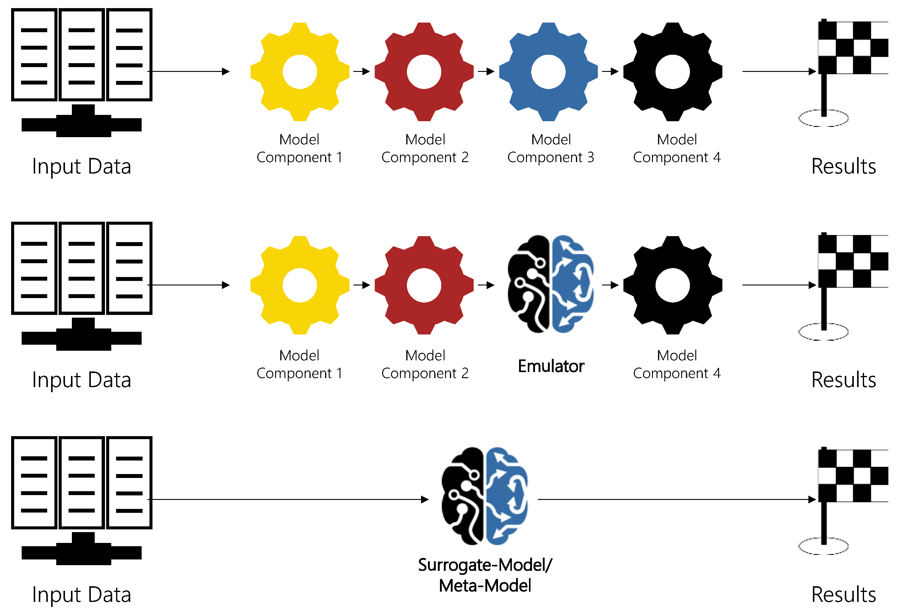
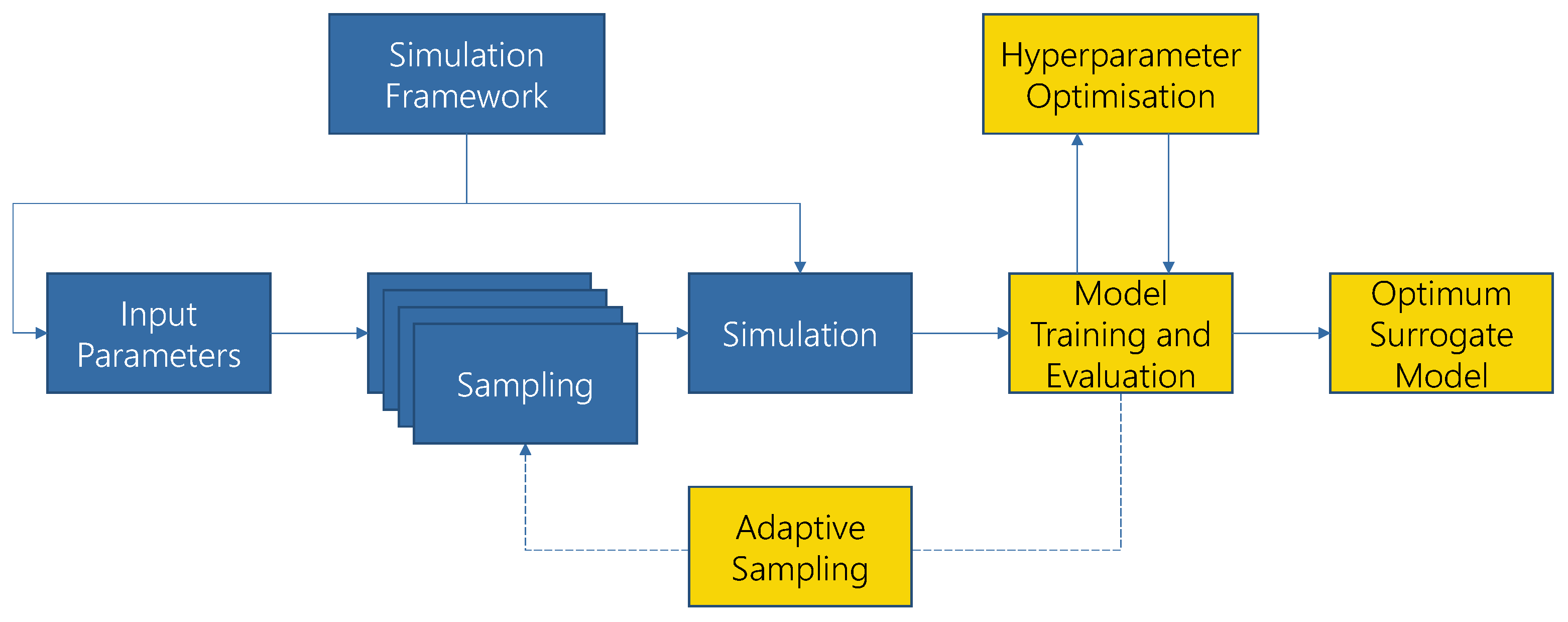
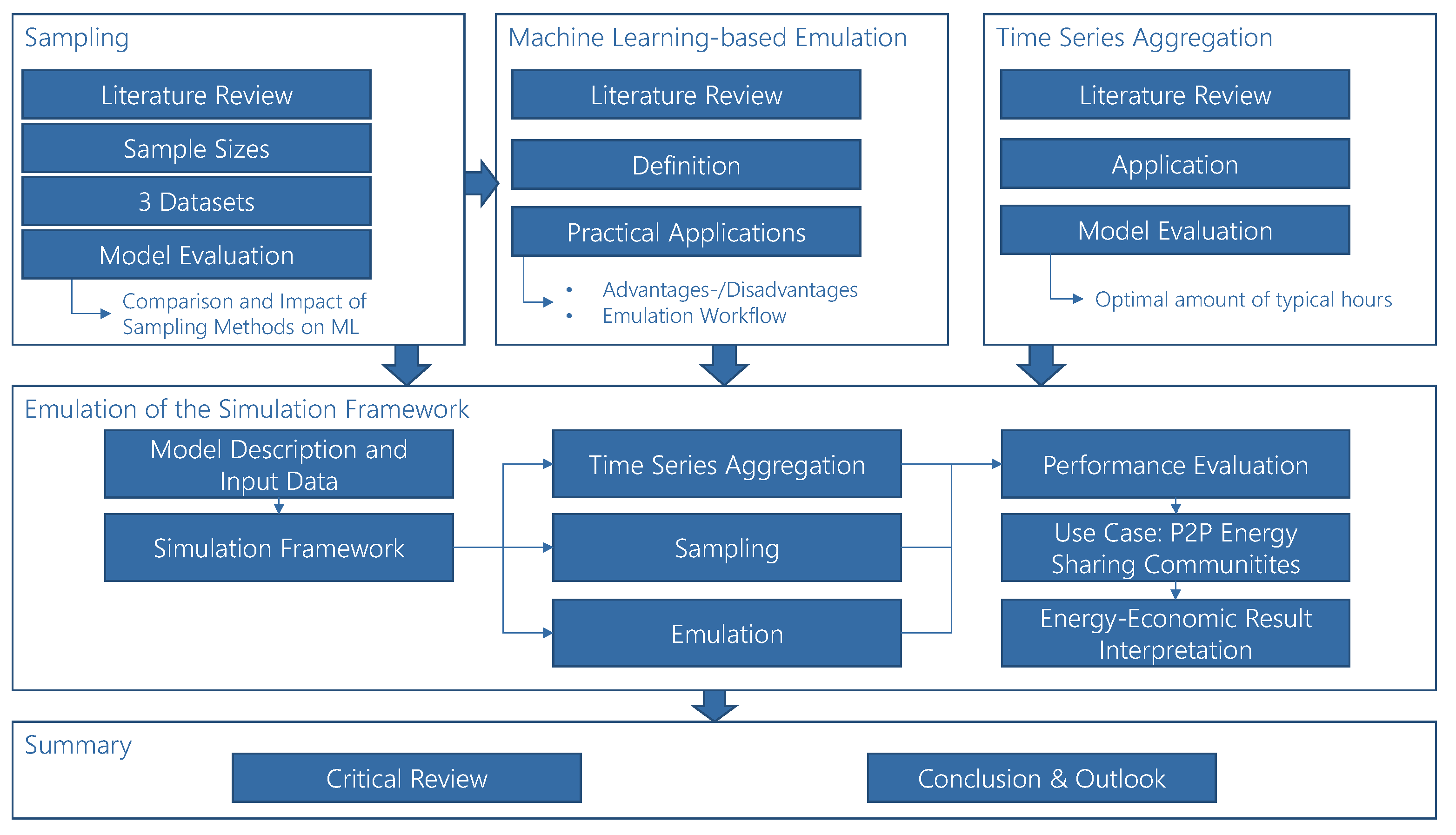
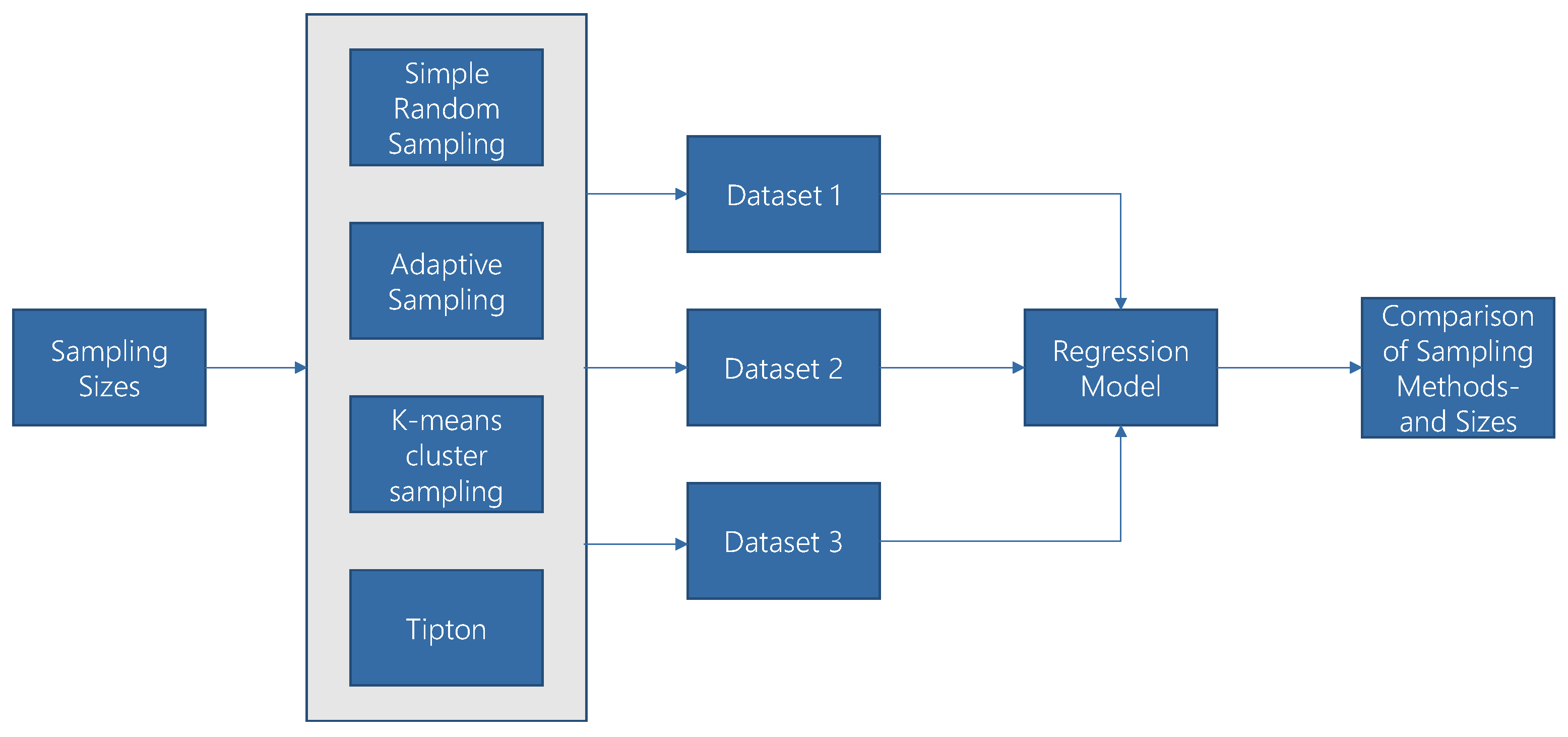
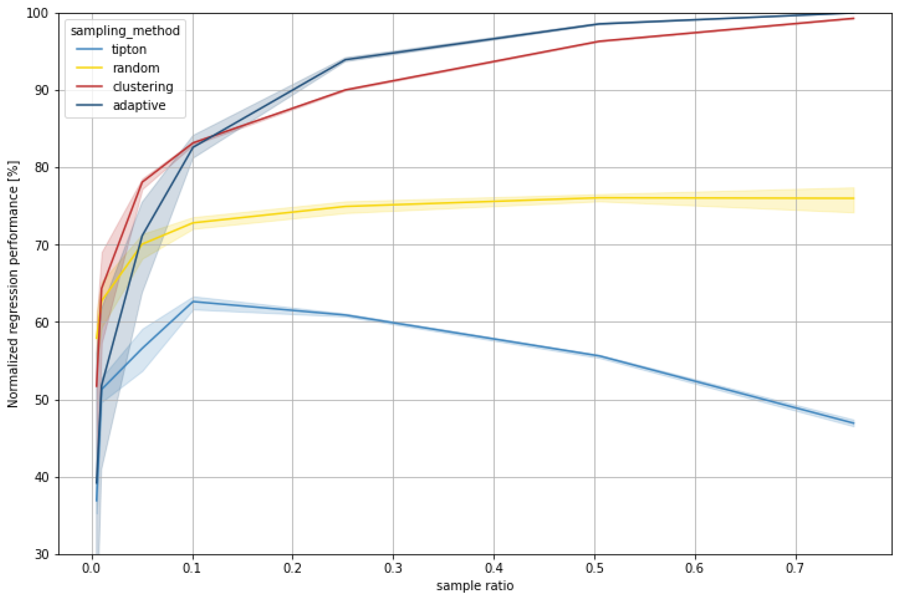
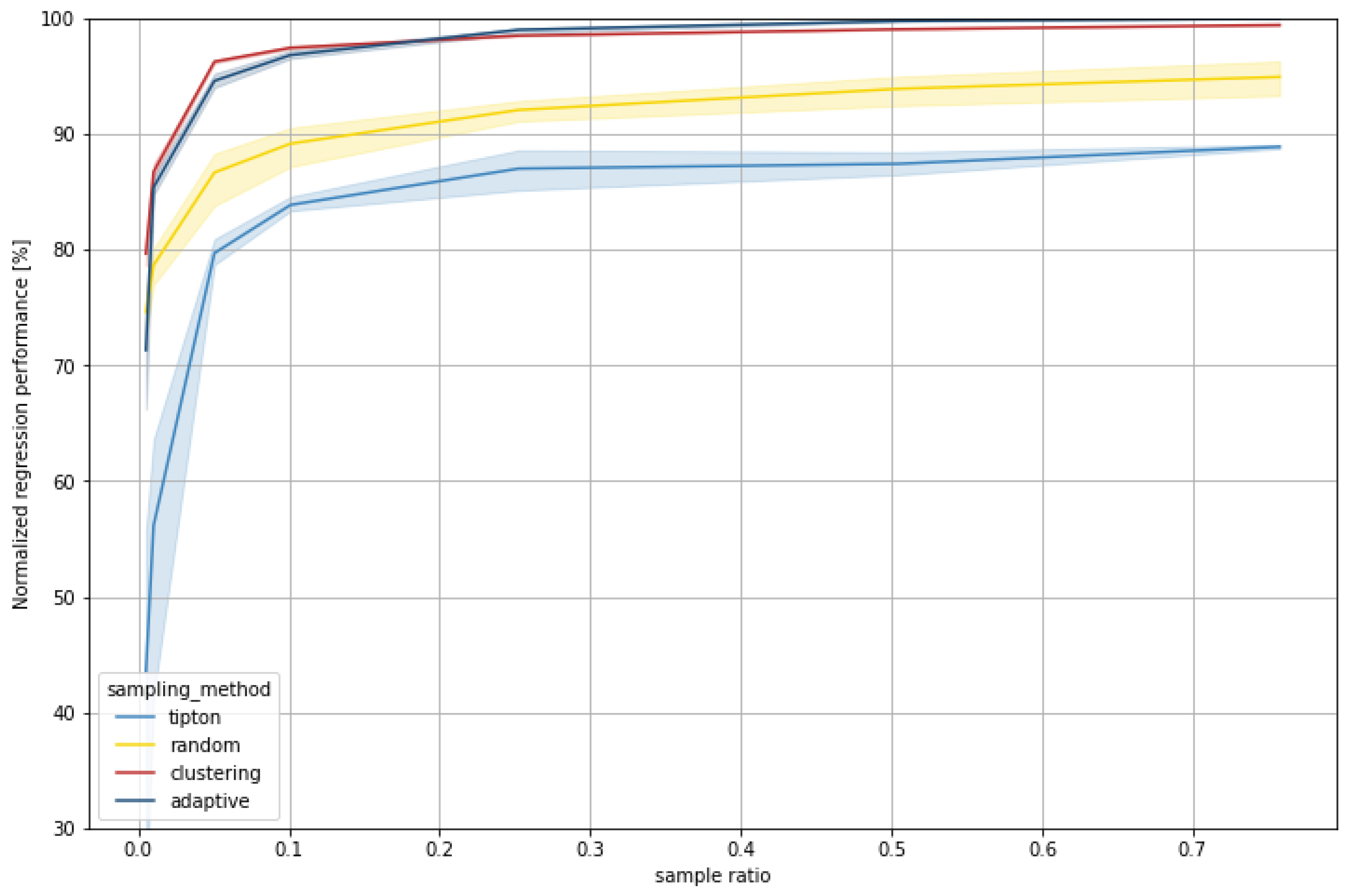
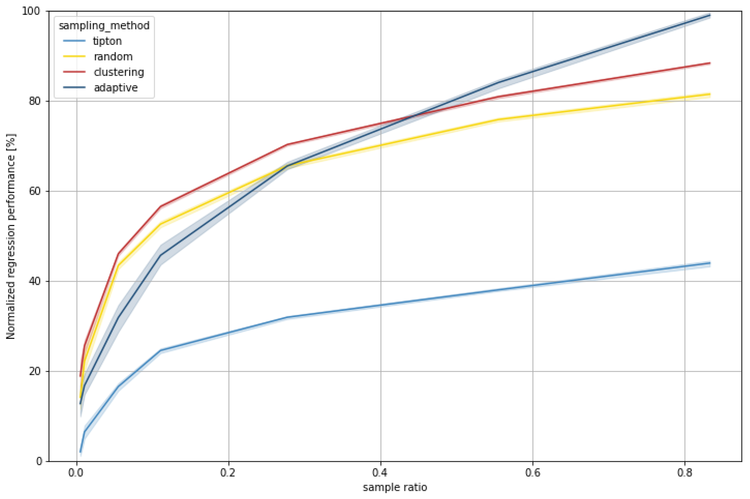
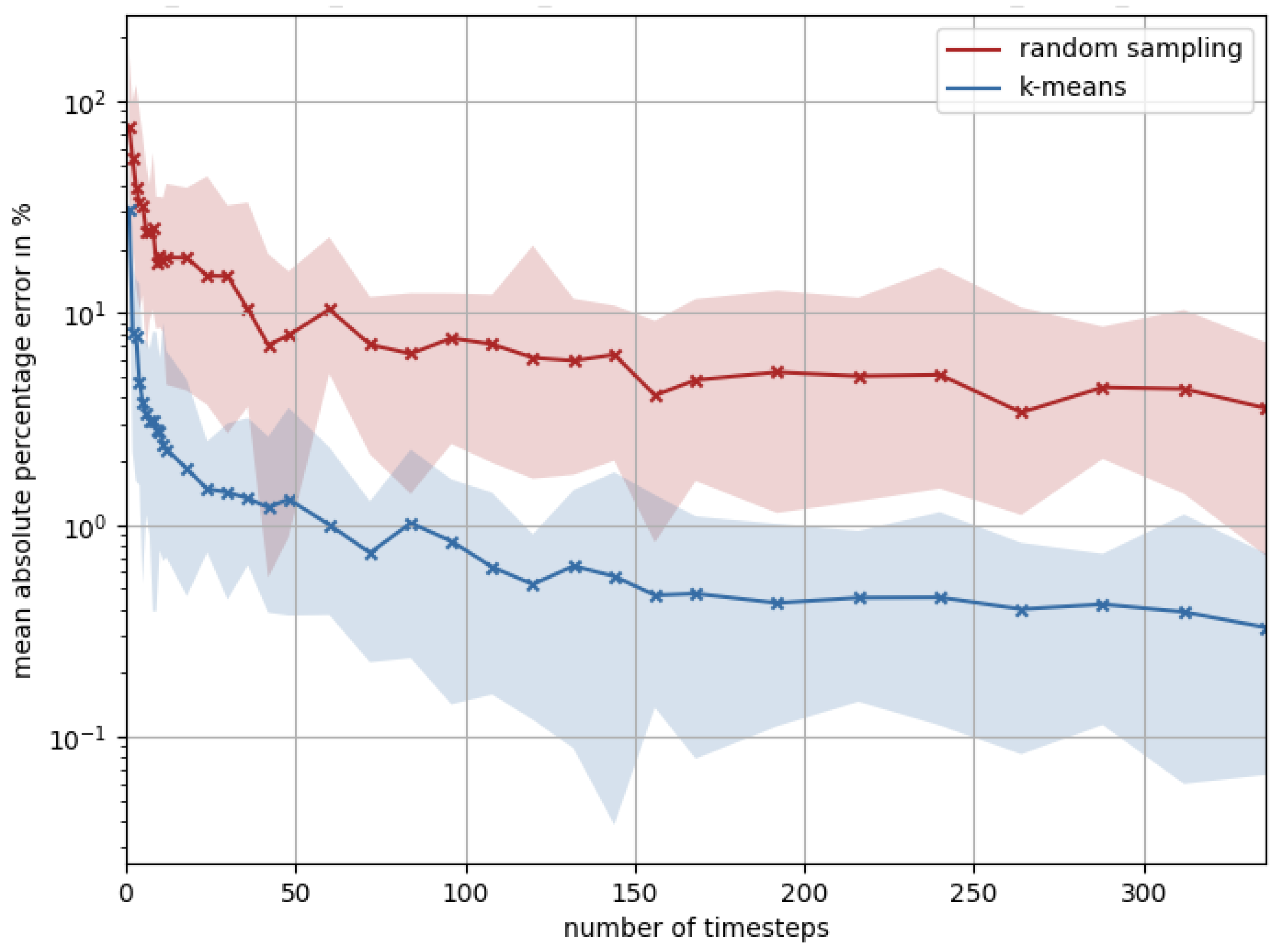
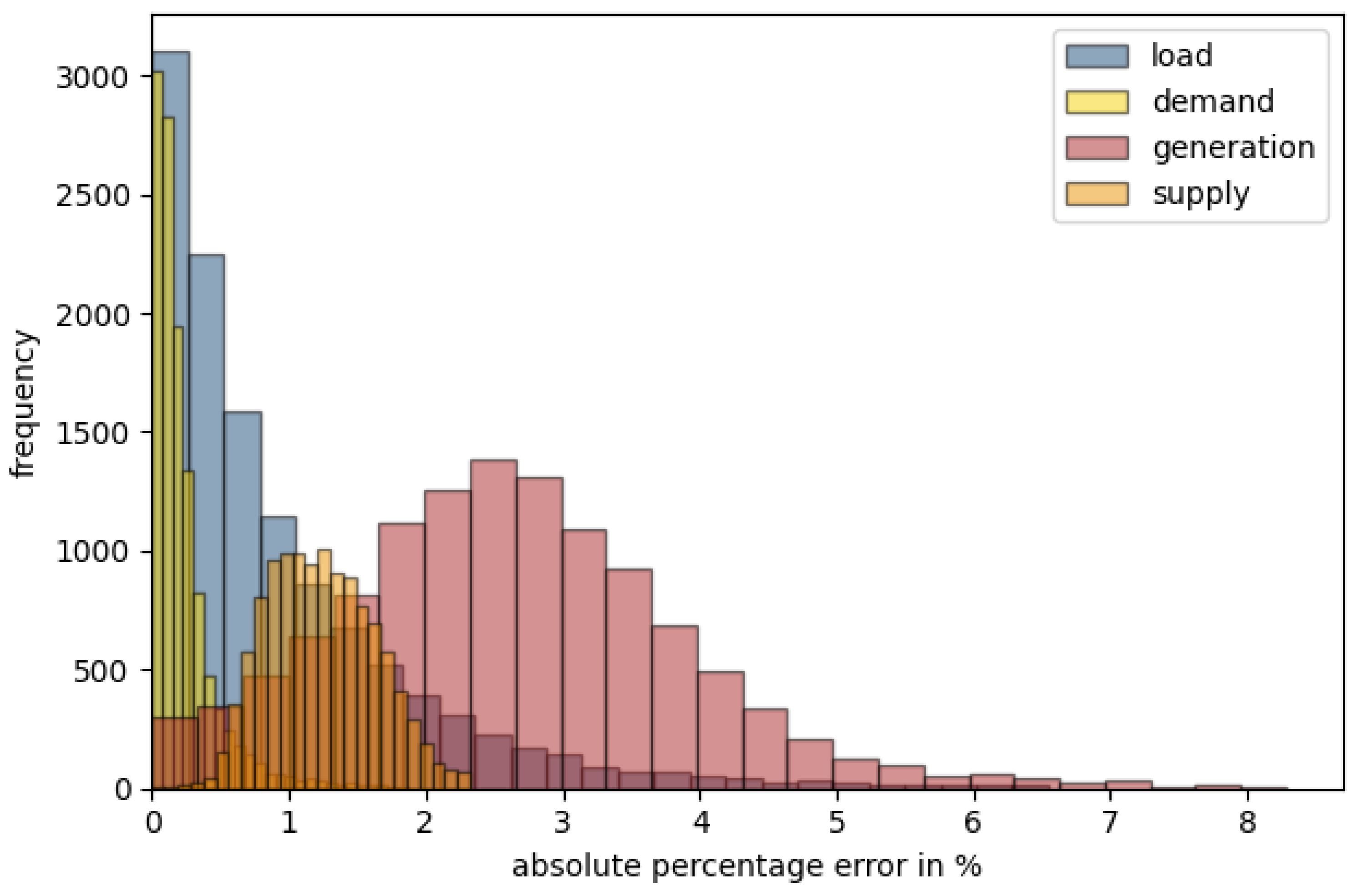
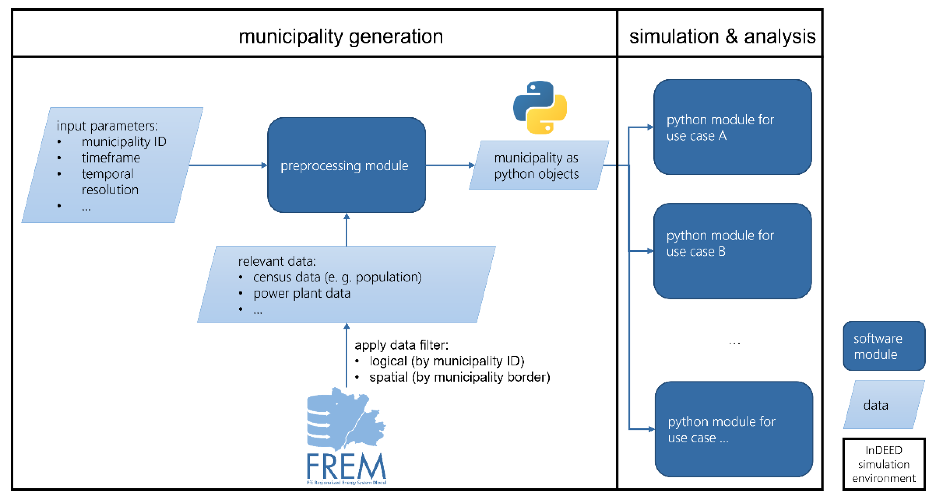
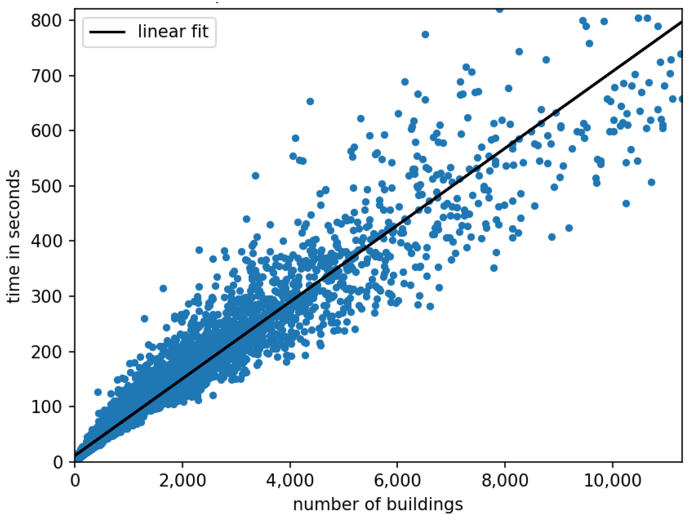
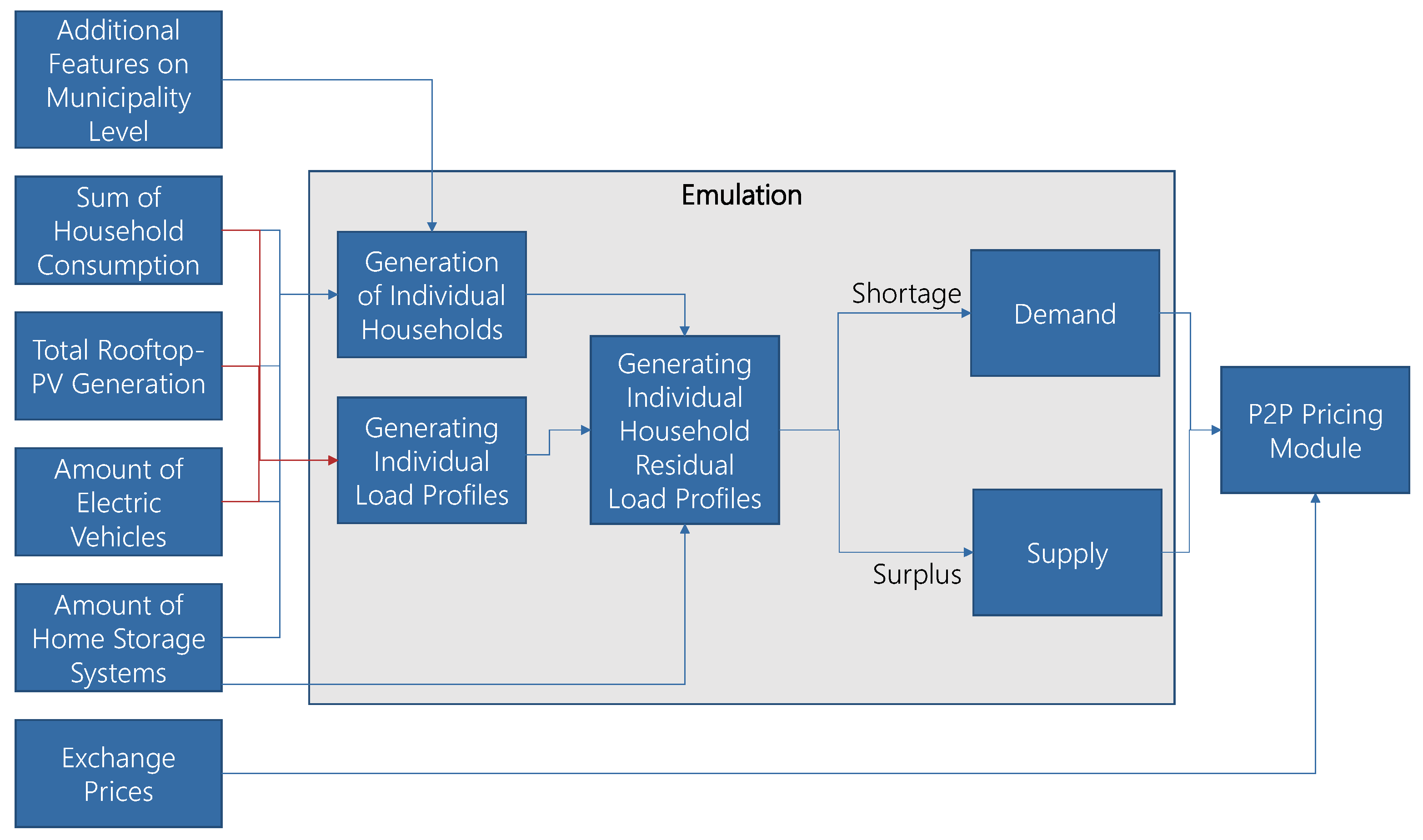
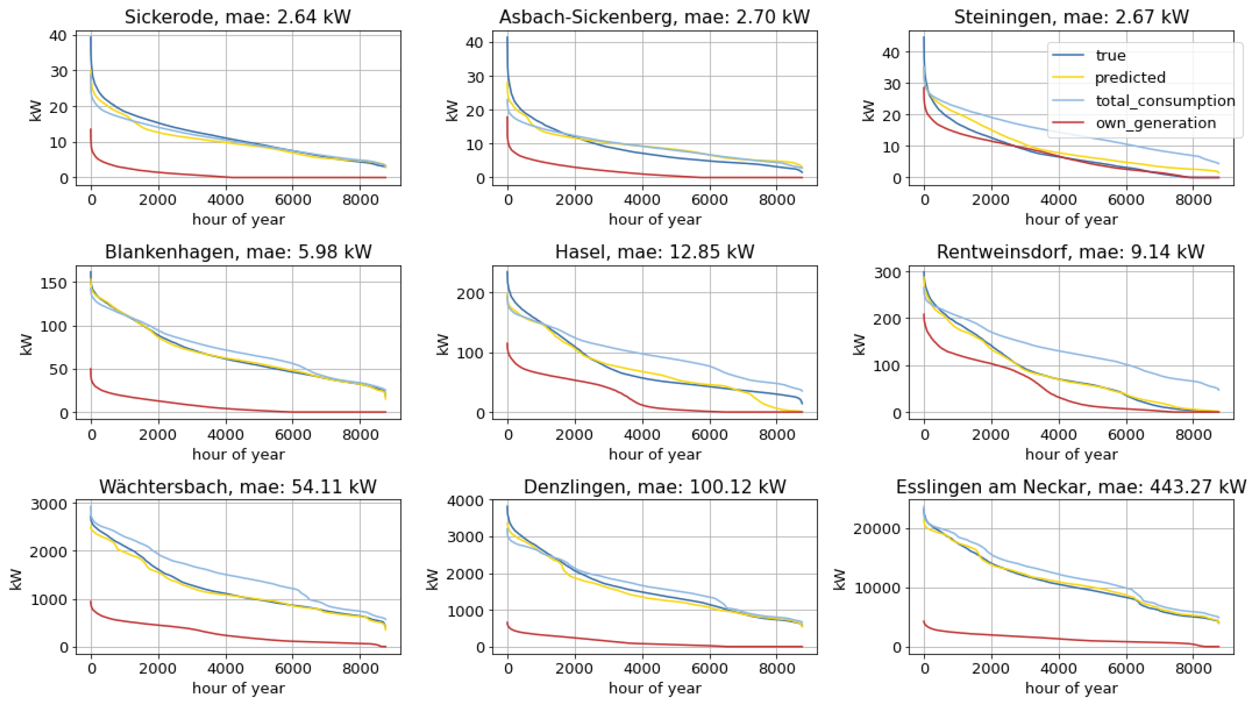
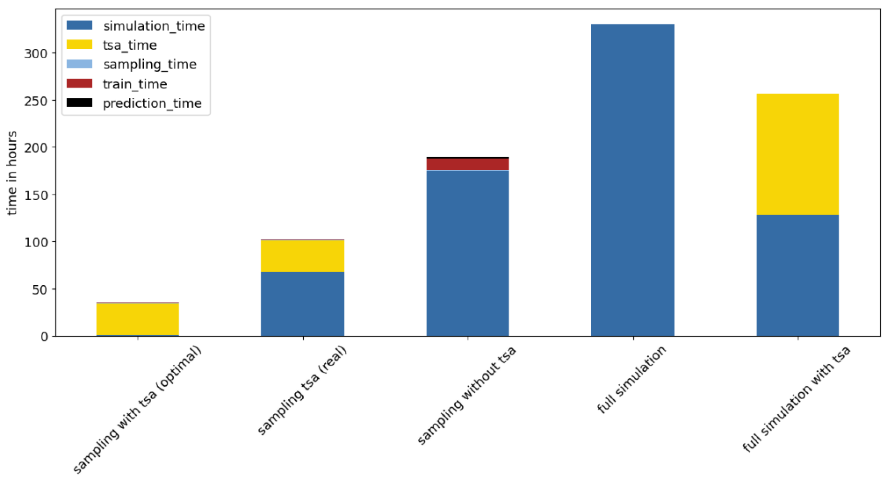
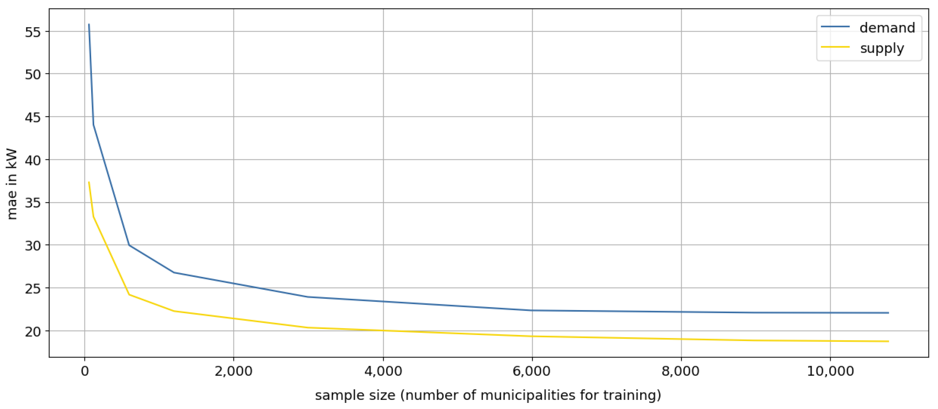
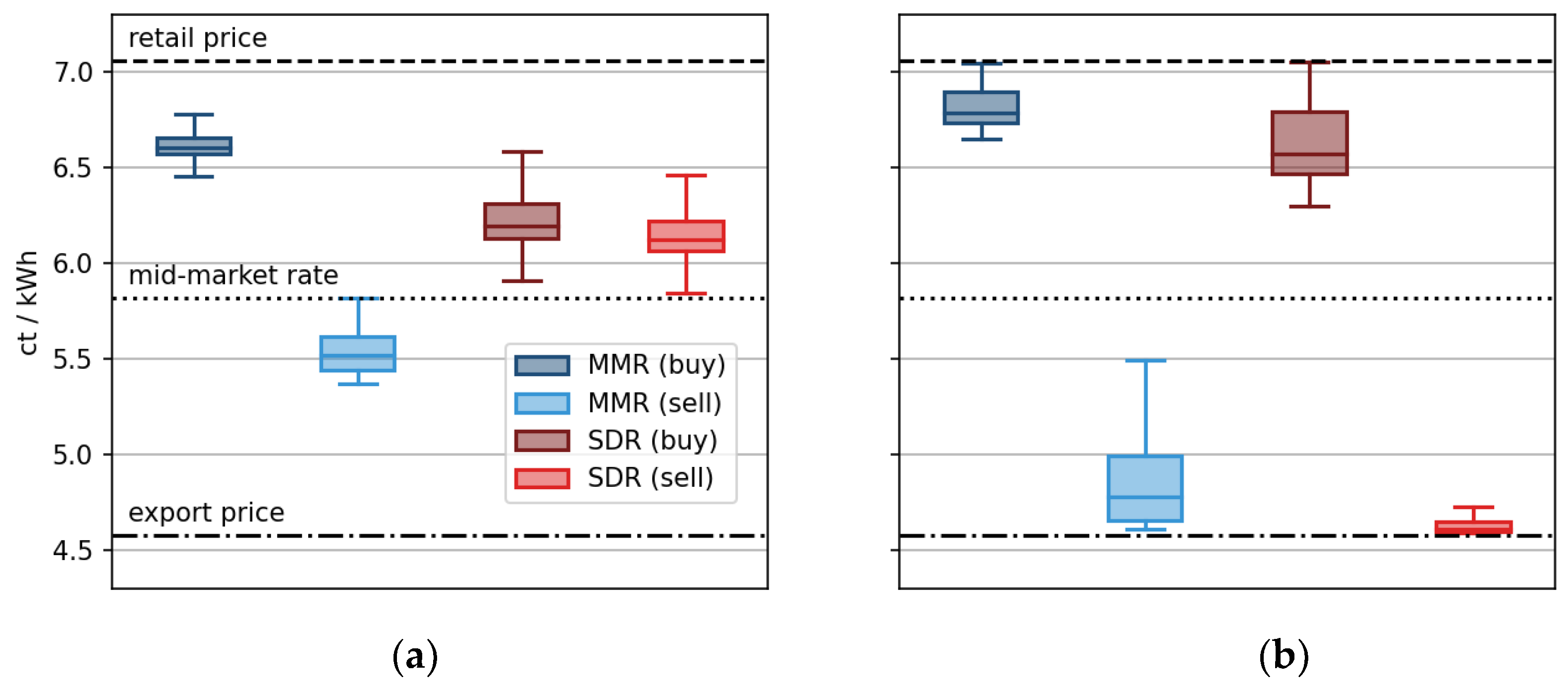
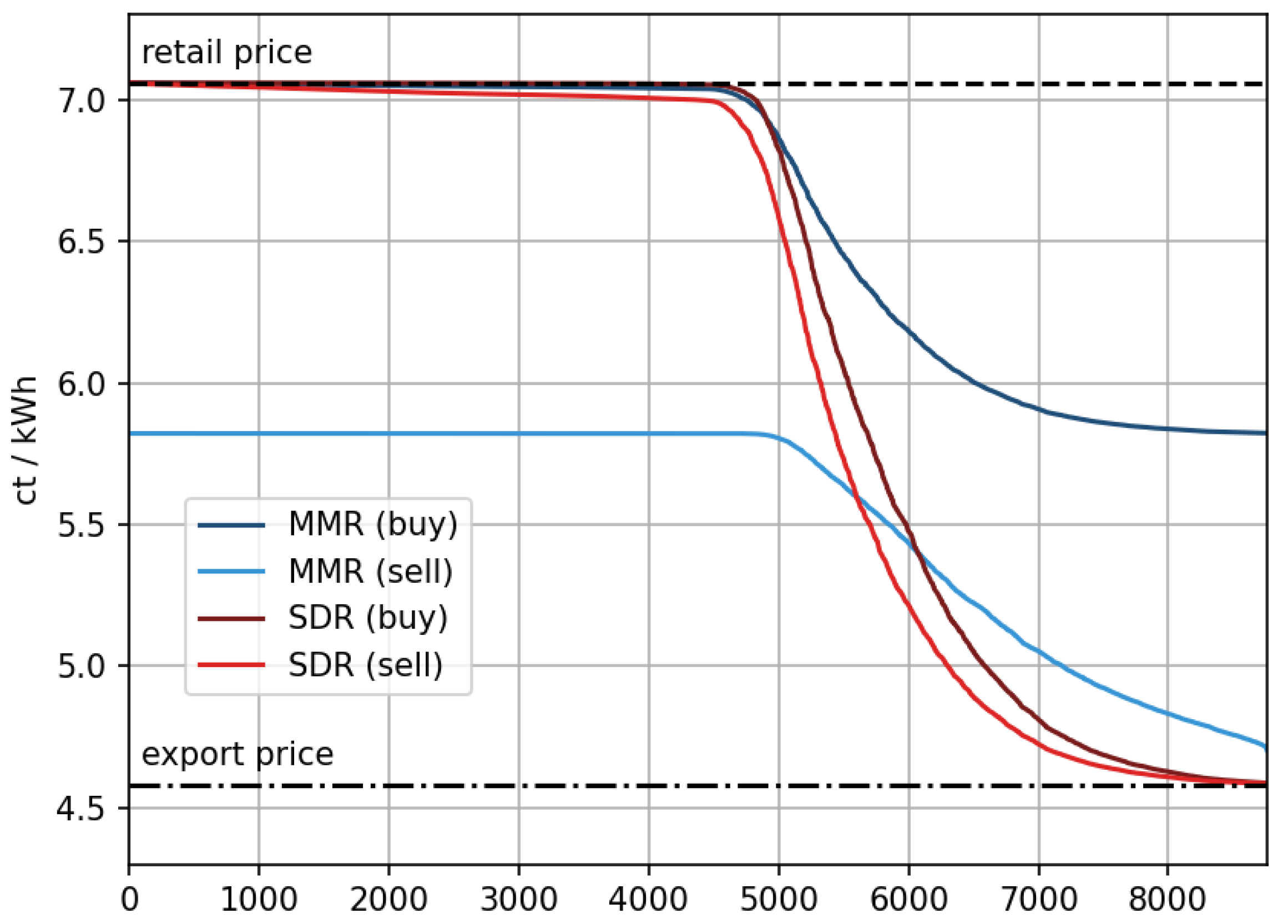
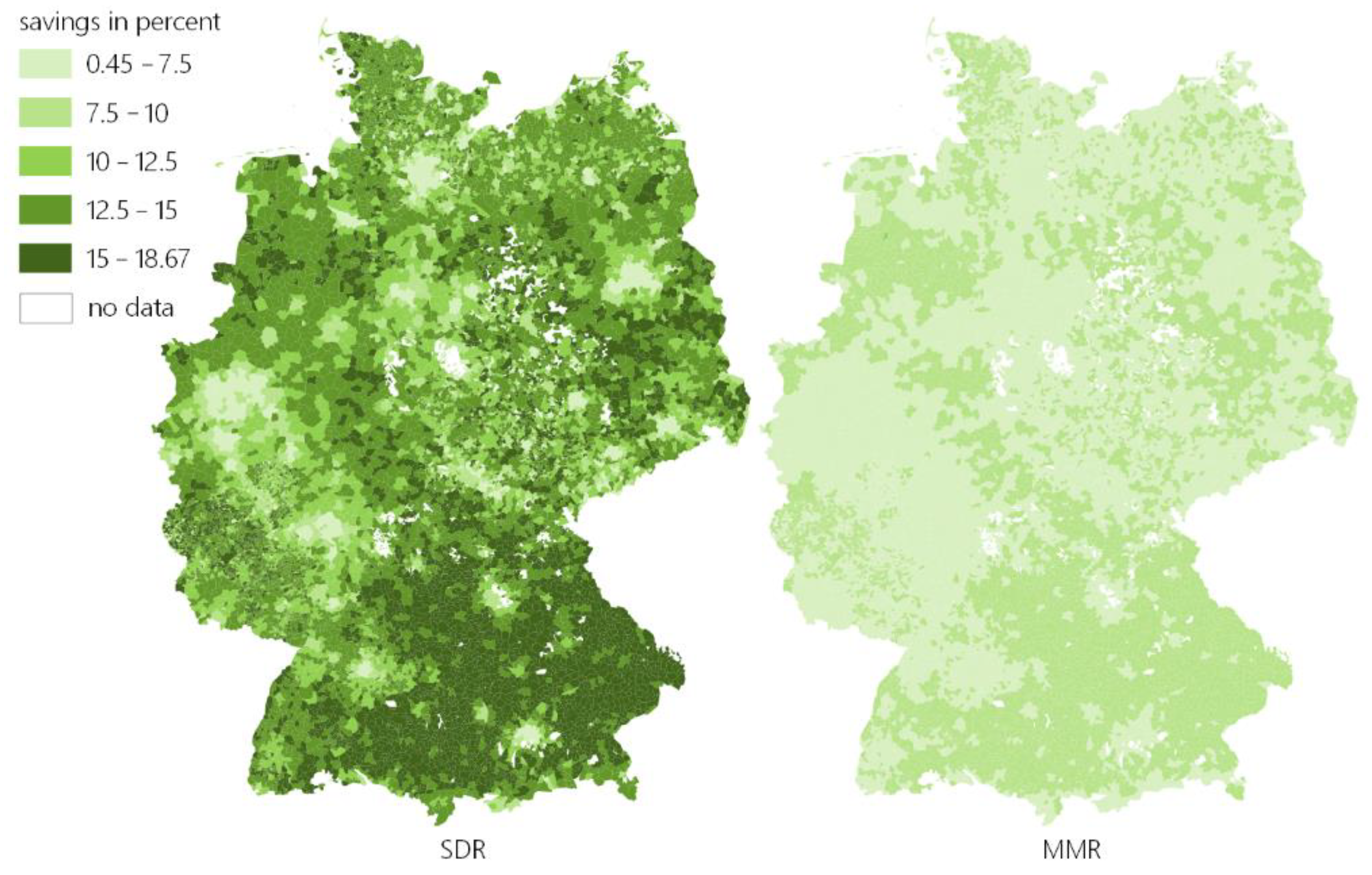
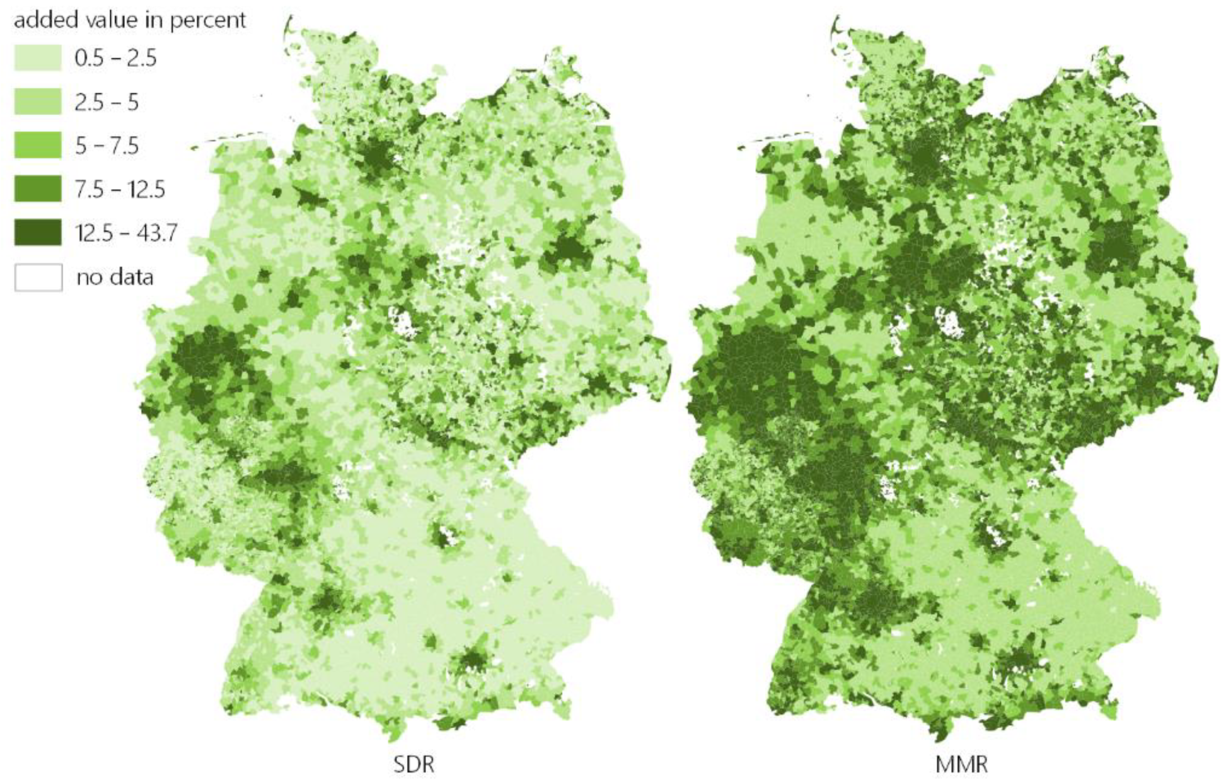
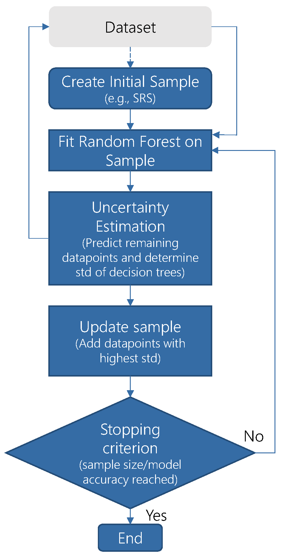
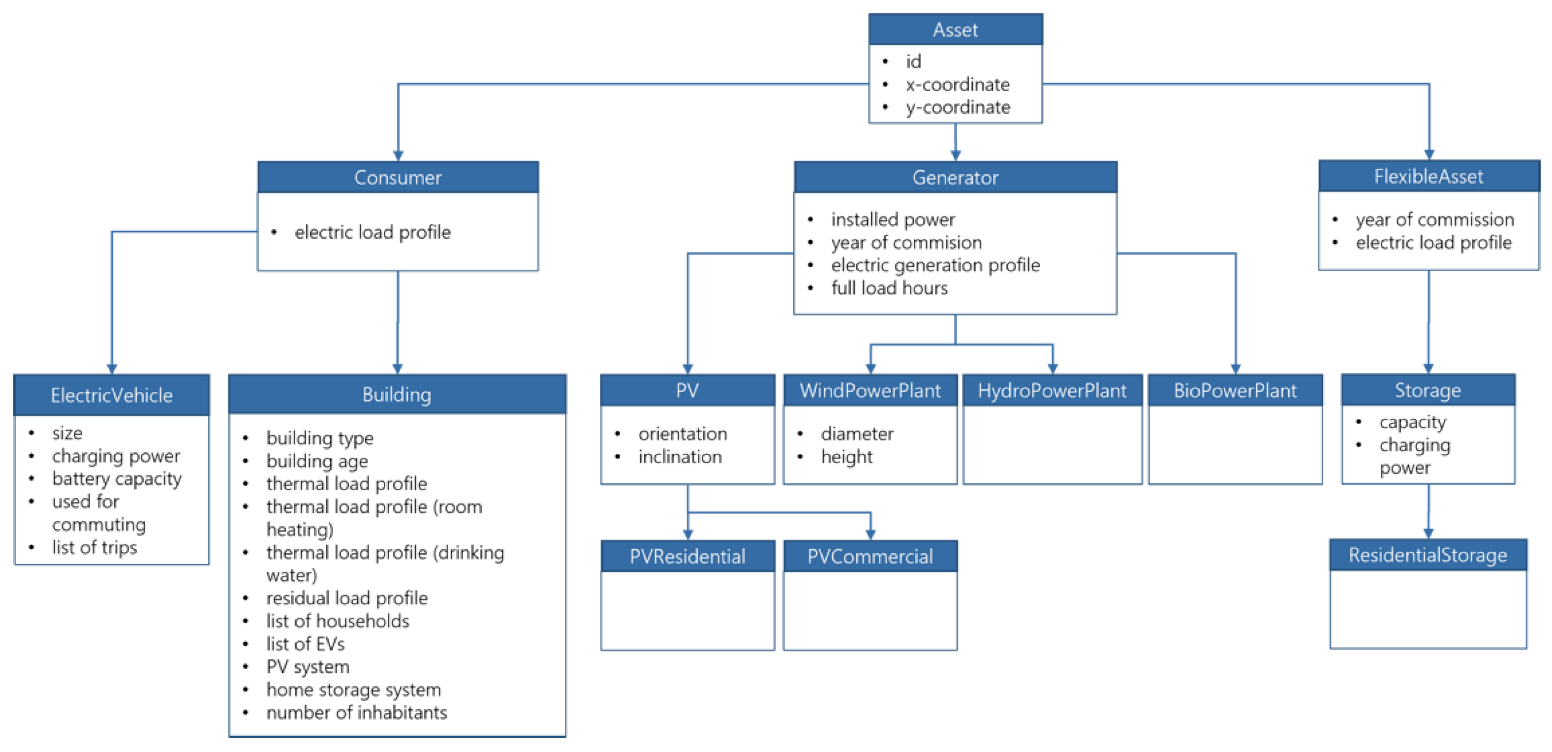
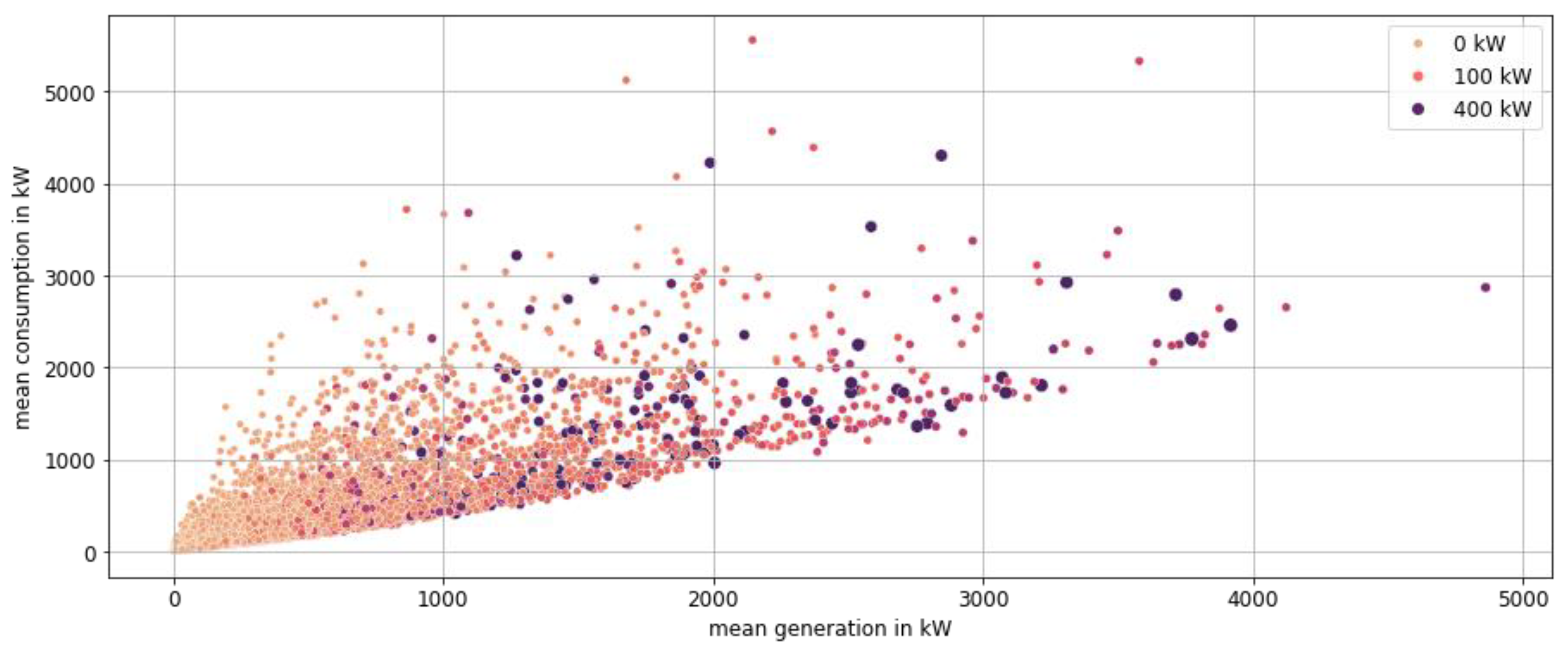
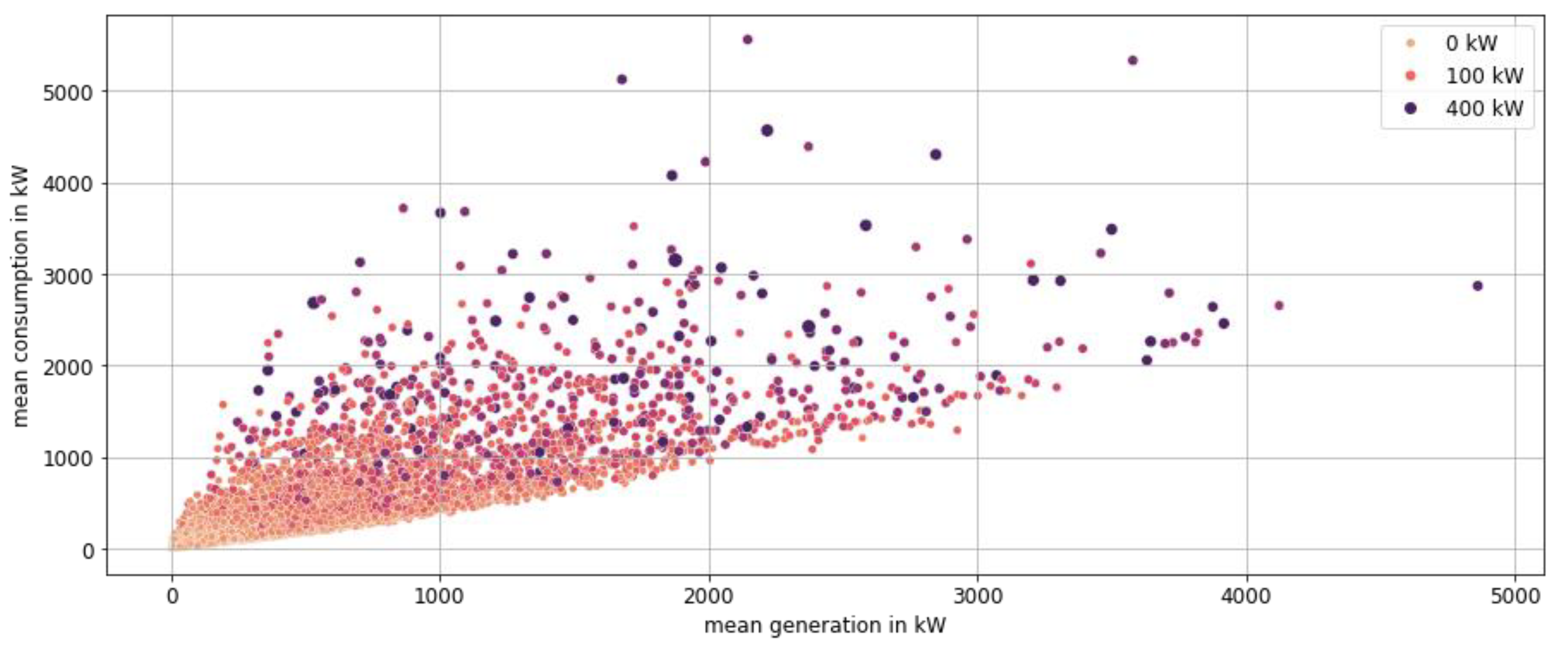


