1. Introduction
Interior permanent magnet synchronous motors (IPMSMs) are increasingly used in household and industrial applications due to their advantages of simple structure, high-torque density, low cost, and good dynamic response [
1]. To guarantee a good driving performance, the output speed of the motor should not only be able to track the reference speed accurately and promptly, but also recover to steady state quickly under the influence of disturbance. The typical filed-oriented control (FOC) topology for IPMSM is designed to be a double-loop structure, where the outer speed loop is in cascade with the inner current loop. Then, the speed and the current can both be controlled through closed-loop regulation. For this control topology, the speed and current regulators play a key role in the performance of the whole IPMSM drive system.
The proportional-integral (PI) control, owing to the advantage of relatively simple structure, high stability, and low steady-state error, is already widely applied in speed and current regulation of IPMSM drives [
2]. However, the IPMSM drive system is a typical nonlinear system. The internal model parameter variations resulting from crossing coupling, magnetic saturation, temperature change, and especially the load inertia change, will induce time-varying and nonlinear characteristics to the model. In this case, the PI control scheme cannot achieve a satisfying dynamic performance in the entire operation range [
3]. To this end, substantial efforts have been devoted to developing nonlinear control schemes, such as sliding mode control [
4,
5], predictive control [
6], robustness control [
7], backstepping control [
8], and artificial intelligence-based control [
9].
The abovementioned control schemes possess their own advantages in handling nonlinear plants. Nevertheless, the various disturbances in the IPMSM drive system still bring challenges for controllers to achieve better performance. In practical applications, IPMSM drive systems are inevitability confronted with various unmeasured disturbances, which may come internally, such as unmodelled dynamics and parameter mismatches, or externally, such as load disturbance. However, the abovementioned schemes are all feedback-based schemes, which means they can only generate the control command through feedback regulation, rather than react directly and promptly to attenuate these disturbances. Although these schemes can finally eliminate the adverse influence of disturbances, it is in a relatively slow way, resulting in the degradation of dynamic performance.
An efficient way to enhance the robustness of the drive system against disturbances and to further exploit the fast dynamic capacities of IPMSM is to introduce an additional feedforward path into the controller besides the traditional feedback path. The newly formulated controller is also known as the two-degree-of-freedom controller [
10], which can counteract the influence of disturbances by using the estimated disturbances to compensate for them in the feedforward path. Among those two-degree-of-freedom methods, active disturbance rejection control (ADRC) shows great prospects due to its unique advantages in handling systems with various uncertainties and disturbance [
11]. The original ADRC is a nonlinear structure with a nonlinear state feedback function, which is designed to achieve a higher convergence rate [
12]. However, this leads to the algorithm being difficult to implement, and makes the stability analysis rather complicated. To this end, Gao simplified this method into a linear version with linear state feedback, known as LADRC [
13]. For the LADRC, the issue of parameter tuning is reduced to the adjustment of bandwidth. Moreover, since the controller is linearized, the conventional frequency-domain method can be adopted to analyze the stability of the controller, which facilitates its application.
In recent years, LADRC has been widely applied in motor drive systems. The LADRC-based regulator can be utilized for current control [
14], speed control [
15,
16,
17,
18], or both [
11,
19,
20]. In [
20], a dual LADRC-based control scheme is proposed, in which the speed LADRC considers the disturbance induced from iron losses, and the current LADRC minimizes the torque ripple by estimating the disturbance corresponding to the back-EMF. In [
21], a higher-order LADRC is studied, in which the conventional dual loop structure is replaced by a single loop structure. Thus, the speed can be directly controlled with faster dynamics. The successful application of LADRC further stimulates the theoretical analysis to go deeper. In [
18], the theoretical comparisons among the PI controller, the disturbance observer (DOB)-based controller, and the LADRC are conducted to show the superiority of LADRC. In [
22], a frequency-domain interpretation of the second-order LADRC is proposed to reveal the association between the LADRC and the PID. In [
23], the relationship between the high-order LADRC and the cascaded low-order LADRCs are explored.
Numerous applications have proved the effectiveness of LADRC in motor control systems. However, for speed control in practical IPMSM drives, there are still some problems that have not yet been fully investigated. Firstly, to achieve closed-loop speed control, the feedback information of rotational speed should be obtained. However, in most application scenarios, the motion sensors mounted on the shaft of the motor are position sensors, such as Hall sensors, optical encoders, or resolvers. Therefore, a low-pass filter is mandatory for suppressing the noise in the process of extracting speed information from the position. Secondly, the rotor magnetic saliency of IPMSM increases the
q-axis inductance and results in a reluctance torque in addition to the permanent magnet torque [
24]. In this case, an MTPA operation scheme is usually adopted to exploit the torque output capability [
1,
25,
26]. Therefore, it would be necessary to improve the conventional LADRC method so as to achieve MTPA operation. Thirdly, to guarantee high performance control of speed, the inertia information of the IPMSM drive system is required. However, in some applications, such as CNC machine tools or winding machines, the inertia may be time-varying. Even though the LADRC can deal with such uncertainties by estimating and compensating for them using linear extended state observer (LESO), it does not mean that the overall performance of the system remains intact. In fact, the kernel of LADRC’s disturbance rejection capability lies in timely and accurate estimation of disturbance. Any mismatch between the actual inertia and the modeled inertia will be regarded as internal disturbance, thereby increasing the estimation burden of LESO, and further degrading the system performance. In [
18], the influence of inertia mismatch on the performance of a surface-mounted PMSM (SPMSM) drive system is discussed. However, the influence of low-pass filter for feedback speed calculation is ignored.
Therefore, to deal with the above mentioned three problems, this article proposes an improved LADRC-based controller for IPMSM drives. The main contributions of this article are summarized as follows.
- (1)
Considering that the typical motion sensor of the IPMSM drive is a position sensor, a third-order LADRC for speed regulation is proposed, in which the position is used as the feedback state. Thus, the low-pass filter for speed calculation can be eliminated.
- (2)
To fully exploit the torque output capability of the IPMSM, the MTPA operation scheme is incorporated into the proposed LADRC-based method.
- (3)
The effect of load inertia mismatch to the system stability, the tracking performance, and the disturbance rejection property is systematically analyzed. To enhance the robustness of the system to inertia mismatch, an inertia identification method is proposed.
- (4)
The proposed LADRC-based method and the load inertia identification method are verified by experimental study.
The remainder of this article are organized as follows.
Section 2 gives a brief description of the dynamic IPMSM model.
Section 3 introduces the design of the LADRC-based speed and current regulators.
Section 4 analyzes the influence of inertia mismatch on the performance of the LADRC-based drive system.
Section 5 presents an improved LADRC-based speed regulator with inertia identification. Finally, the experimental results are shown in
Section 6, and the conclusions are drawn in
Section 7.
2. Dynamic Model of IPMSM
To simplify the modeling of IPMSM, it is commonly assumed that the employed IPMSM has negligible magnetic saturation, cross-coupling, iron losses, and eddy current losses. Moreover, the three-phase windings are symmetric, and the magnetic field in the airgap is sinusoidal. Thus, the stator current dynamics of IPMSM can be described in the
d-
q synchronous reference frame as:
and the mechanical motion dynamics is described as:
where
and
are the
d-
q-axis stator currents;
and
are the
d-
q-axis stator voltages;
and
are the
d-
q-axis inductances;
is the stator winding resistance;
is the flux linkage of the permanent magnet;
is the number of pole pairs;
is the rotor angular velocity (rad/s);
is the viscous friction coefficient (N·m·s/rad);
is the moment of inertia (kg·m
2);
is the load torque (N·m); and
is the electromagnetic torque (N·m). For the employed IPMSM,
is expressed as:
It can be seen in Equation (3) that the electromagnetic torque is comprised of two terms. The first term is the permanent magnet torque . The second term is the reluctance torque which is proportional to . To fully utilize the reluctance torque, the MTPA operation scheme should be incorporated into the controller.
3. Design of LADRC-Based Speed and Current Regulators with MTPA Scheme
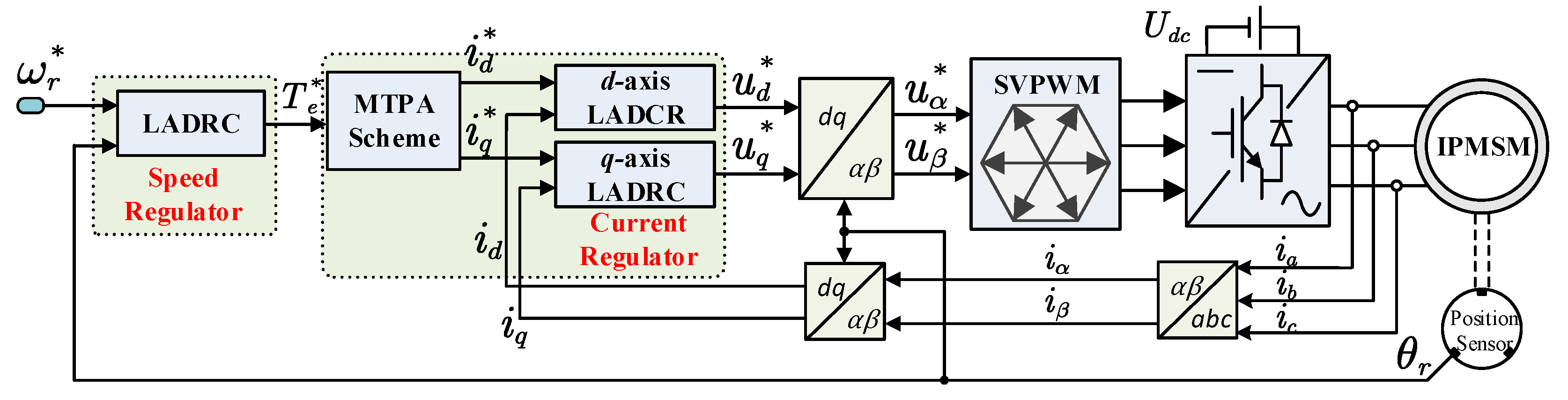
The LADRC-based IPMSM drive system with an MTPA scheme is shown in
Figure 1. The overall system is comprised of an IPMSM, a position sensor, a three-phase voltage-source inverter, a SVPWM generator, three coordinate transformation modules, a speed regulator, and two current regulators. Under the field-oriented control topology, the three-phase stator currents are transformed into
d-axis and
q-axis currents, which respectively represent the flux-producing component and the torque-producing component. The control loop includes a speed loop and two current loops. The speed regulator generates the torque reference, the MTPA scheme generates the
d- and
q-axis current references according to the torque reference, and the two current regulators generate the
d- and
q-axis voltage references.
The speed and current regulators play a key role to the performance of the IPMSM drive system. In this section, a synthesized design for LADRC-based speed and current regulators is presented.
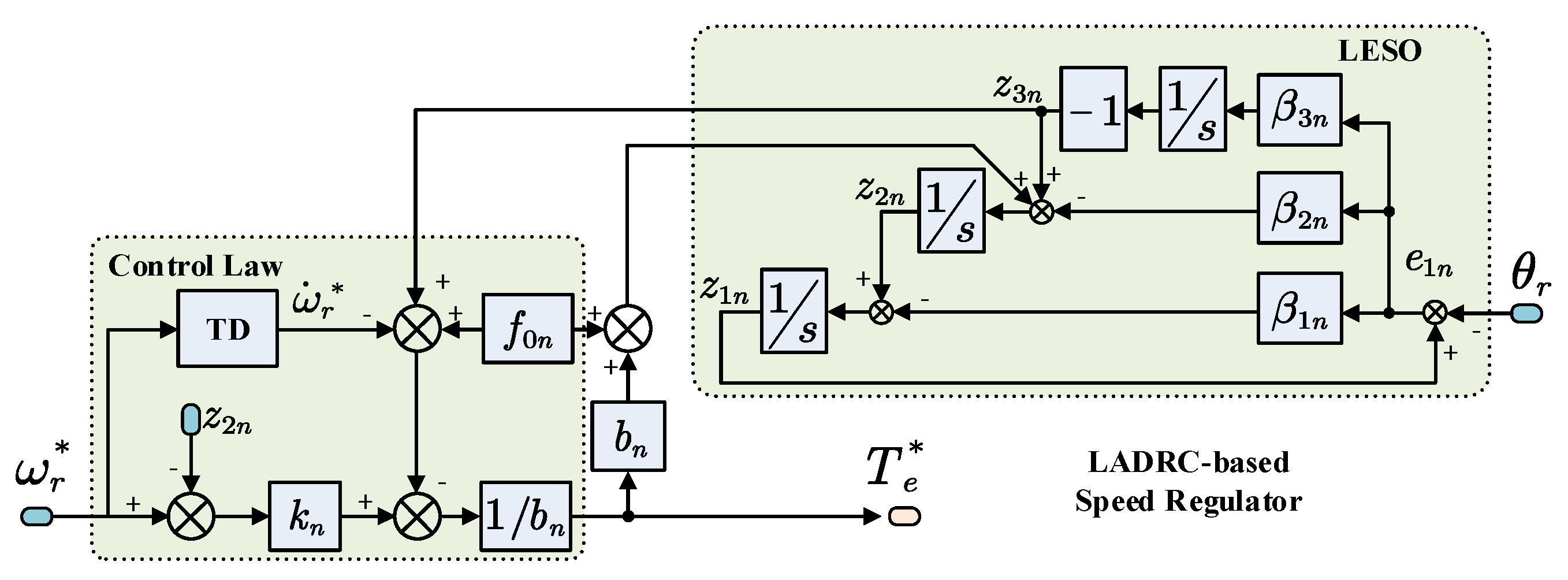
3.1. Design of LADRC-Based Speed Regulator
The key to the application of LADRC is to reformulate the practical controlled plant to a cascaded integral plant and to achieve the modelling of disturbance [
11]. To design the speed LADRC, the mechanical motion dynamics of the IPMSM are reformulated as:
where
is the torque reference;
is the critical gain and
;
and
are respectively the known disturbance and the unknown disturbance; the sum of
and
represents the total disturbance;
is the estimated value of angular velocity; and
is the other unknown disturbance, such as unmodeled dynamics and noise.
In Equation (4), the unknown disturbance is distinguished from the known disturbance . It can be seen that consists of the load torque term and the difference term ( and ). Therefore, the load torque fluctuation and the sudden speed variation will both be considered in the disturbance model.
Commonly, for the first-order plant presented in Equation (4), a second-order LESO can be designed by regarding
as the extended state variable. However, the second-order LESO requires speed feedback information. For most application scenarios, the motion sensors mounted on the shaft of the motor are position sensors, such as Hall sensors, optical encoders, or resolvers. Therefore, the speed information cannot be directly obtained. In order to extract the speed from the measured position, a low-pass filter is required to suppress the noise induced from derivate operation, i.e.,
, where
is the measured rotor position. To eliminate the filter, the second-order plant can be adopted:
Then, a third-order LESO is designed to estimate the states and the unknown disturbance by using the position feedback instead of speed feedback:
where
,
,
are the estimations of
,
,
;
is the estimation error of LESO; and
,
,
are the observer gains. For convenience of parameter tuning and theoretical analysis, this article adopts a scaling- and bandwidth-parameterization method [
13]. The gains are parameterized as follows:
where
is a positive constant denoting the bandwidth of LESO. A higher
helps improve the response rate, but will increase the observer’s sensitivity to noise. In practical applications,
should be designed within reason so as to reach a tradeoff between the rapidity of estimation and the immunity to noise.
The LESO presented in Equation (6) only requires position information . The rotor speed is estimated through the observer, i.e., . Therefore, the low-pass filter used for speed calculation is eliminated.
When LESO becomes stable, the estimation error
will converge. The speed tracking error of LADRC is defined as
. Then, the tracking error dynamic equation can be expressed as:
By adopting the linear feedback control, the speed tracking error will converge in exponential form:
where
is the proportional gain. By substituting Equation (9) into Equation (8), the control law of speed loop LADRC can be derived as:
The control law presented in Equation (10) requires the derivative of reference speed as input. This derivative term acts as a feedforward term to track the variation of reference speed, thereby diminishing the oscillation and overshoot during the adjustment of speed. In practical applications, a tracking differentiator (TD) [
12] can be adopted to calculate
. The block diagram of the LADRC-based speed regulator is shown in
Figure 2.
3.2. Design of LADRC-Based d-q-Axis Current Regulator with MTPA
3.2.1. d-q-Axis Current Reference Generation Based on MTPA Scheme
The essence of controlling the torque is to control the
d- and
q-axis currents. In the dual loop control structure, the speed regulator generates the torque reference
. Therefore, it is necessary to obtain the
d-
q-axis current reference according to
. Commonly, the
d-axis current reference is set to zero, so that the
q-axis current reference will be proportional to
. However, the rotor magnetic saliency of the IPMSM increases the
q-axis inductance and results in a reluctance torque in addition to the permanent magnet torque. To fully exploit the torque output capability of the IPMSM, the maximum torque per ampere (MTPA) operation scheme is adopted. The goal of the MTPA scheme is to achieve the desired torque with a minimum stator current
required, thereby reducing the copper losses and improving the efficiency. The constraints between
,
, and
under MTPA operation is given by:
The proof for Equation (11) is presented in the
Appendix A. For any given torque reference, the
d- and
q-axis current references required for MPTA operation can be obtained from Equation (11). However, the explicit solution of
and
cannot be derived, which makes Equation (11) unsuitable for real-time implementation using microprocessors. To reduce the computation burden, the MTPA scheme can be implemented by means of look-up tables (LUT) with offline calculations [
26]. In this article, the LUT method is adopted to achieve MTPA operation.
3.2.2. Current Regulator Design
The current regulator plays a key role in the torque performance of IPMSM. To design the LADRC-based current regulator, the current dynamics of IPMSM are reformulated as:
where
and
are the
d-
q-axis stator voltage references;
and
are the critical gains, and
,
;
and
are respectively the known disturbance and the unknown disturbance of the
d-axis; and
and
are respectively the known disturbance and the unknown disturbance of the
q-axis.
and
are the other unknown disturbance such as unmodeled dynamics and noise.
By regarding the unknown disturbance
and
as the extended states, the second-order LESOs for
d-axis and
q-axis are established:
where
,
,
,
are the estimations of
,
,
,
;
,
are the estimation errors of LESO; and
,
are the observer gains which are parameterized as follows:
where
is the bandwidth of the current loop LESO.
In analogy with Equation (10), the control law of current loop LADRC can be derived as:
where
and
are the proportional gains for the
d- and
q-axes. The block diagram of the LADRC-based
d-
q-axis current regulators are shown in
Figure 3.
4. Speed Response of the Drive System in the Presence of Inertia Mismatch
The above designed LADRC-based IPMSM drive system requires information on the machine parameters. In particular, the accuracy of the rotor inertia is highly related to the performance of the speed loop. In some applications, such as CNC machine tools or winding machines, the inertia may be time-varying. Although the LADRC can deal with such uncertainties by estimating and compensating for them by using LESO, this does not mean that the overall performance of the drive system remains intact. In fact, the kernel of LADRC’s disturbance rejection capability lies in timely and accurate estimation of disturbance. Any mismatch between the actual inertia and the modeled inertia will be regarded as internal disturbance, thereby increasing the estimation burden of LESO, and further degrading the system performance. In this section, the speed response of the LADRC-based IPMSM drive system in the presence of inertia mismatch are analyzed in detail.
4.1. Frequency-Domain Derivation of the Speed Response
Considering the inertia mismatch, the LESO and the control law of speed loop LADRC are rewritten as:
where
and
are the estimated value of
and
. Then, by transforming Equation (19) into the frequency-domain, the following transfer functions are obtained:
where
is the characteristic polynomial of LESO,
. It should be noted that a lowercase letter is used to represent a time-domain variable, whereas the corresponding capital letter is used to represent the variable in the frequency-domain, e.g.,
and
.
By transforming Equation (20) into the frequency-domain, and combining it with Equation (21), we obtain:
where
,
.
Then, transforming Equation (5) into the frequency-domain, and combining it with Equation (22), we obtain:
Defining
to denote the mismatch ratio of inertia, Equation (23) is rewritten as:
where
is the characteristic polynomial of the closed-loop control system:
Apparently, Equation (24) denotes the speed response with respect to the reference speed and the unknown disturbance in the presence of inertia mismatch. By conducting the frequency-domain analysis, the speed control performance of the LADRC-based drive system can be evaluated.
4.2. Influence of rb on Closed-Loop Stability
To analyze the influence of on the closed-loop stability of the system, the generalized root locus method is adopted. The main idea of this method is to create a new system which owns the same closed-loop characteristic polynomial as Equation (24), and the open-loop gain of the new system is . Then, by analyzing distribution of the open-loop zeros and poles of the new system, the closed-loop stability of system Equation (24) can be indirectly investigated.
Firstly, letting the left side and right side of Equation (25) both be divided by
, and separating
from the equation:
Then, the open-loop transfer function of the new system is designed as:
By setting
, and
(
,
,
) as an example, the root locus plot of Equation (27) with respect to
is obtained, as shown in
Figure 4.
The poles and zeros have been labeled in
Figure 4. It can be seen that, if
, a pair of conjugate complex poles are located on the right side of the imaginary axis, which indicates that the system is unstable. To study the influence of
on the closed-loop stability in a more specific way, the separation points of the root locus and the intersection points with imaginary axis are derived in the following. Firstly, let:
The separation points of the root locus and the corresponding
are derived:
The intersection points of root locus with the imaginary axis and the corresponding
are derived:
It can be easily proved that
,
. Therefore, according to
Figure 4 and Equations (29) and (31), the following conclusions can be drawn:
- (1)
If , a pair of conjugate complex poles are located on the right side of the imaginary axis, thus the system is unstable.
- (2)
If , there exists a pair of conjugate complex poles and a real dominant pole. However, if is very close to , the real part of the complex poles would be very small, and the imaginary part would be very large, thus the overshoot of the system’s step response would be very significant.
- (3)
If , all poles are located on the real axis, thus the step response has no overshoot. Moreover, a larger leads to a faster step response.
- (4)
If , there exists two pair of conjugate complex poles, the system is always stable in this region, and the overshoot exists but is not significant.
4.3. Influence of rb on Tracking Performance
According to Equation (24), the transfer function of speed with respect to its reference is described as:
Setting
, and
(
,
,
) as an example, the Bode diagram of the transfer function
is shown in
Figure 5.
Figure 5 demonstrates the speed tracking performance of the LADRC-based drive system under different
. It can be seen that if
, the system has the desired speed tracking performance in the whole frequency range. If
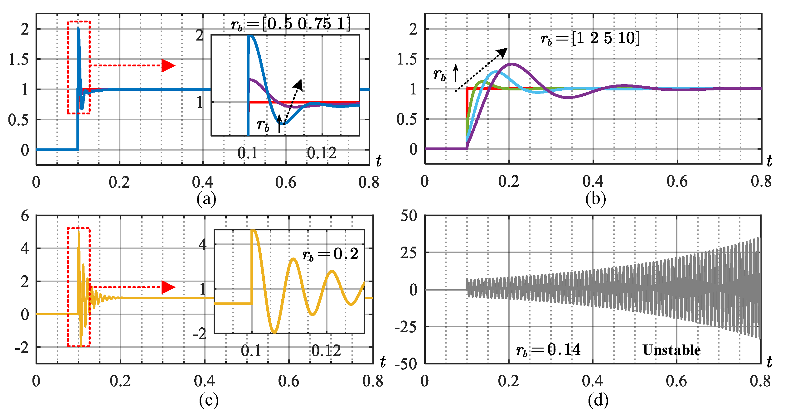
, a steady-state tracking error will occur in the medium- and high-frequency range. However, in the low-frequency range, where the reference speed varies slowly, the steady-state tracking error is negligible. Therefore, it is concluded that the tracking performance of the LADRC-based drive system against inertia mismatch decreases as the frequency of the reference increases.
Figure 6 shows the step response of the transfer function
under different
. It can be noted that the system will not achieve the desired response as long as
. If
is too small, the step response will diverge, hence the system will be unstable. These results are in accordance with the above frequency analysis.
4.4. Influence of rb on Disturbance Rejection Performance
According to Equation (24), the transfer function of speed with respect to the unknown disturbance is described as:
Figure 7 demonstrates the disturbance rejection performance of the LADRC-based drive system under different
. It can be noted that as long as the system is stable, i.e.,
, the disturbance rejection performance increases as
decreases. Moreover, under the same
, the disturbance rejection performance in the medium-frequency range is relatively weaker than that in the low- or high-frequency range.
Figure 8 shows the step response of the transfer function
under different
. It can be noted that as long as the system is stable, the external step unknown disturbance will be quickly rejected by the LADRC. The overshoot decreases as
decreases, which means that the disturbance rejection performance increases. These results are in accordance with the above frequency analysis. Finally, it is concluded that the overestimation of inertia, i.e.,
, is beneficial for the disturbance rejection performance of the LADRC.
According to the above analysis, it can be found that the inertia mismatch can significantly influence the performance of the LADRC-based drive system. Small , i.e., overestimated inertia, can enhance the disturbance rejection performance to a certain degree, but may lead the system to be unstable. As for the tracking performance, it is found that the system will not achieve the desired response as long as . Therefore, to obtain a good tracking performance as well as guarantee the system’s stability, it is necessary to identify the load inertia.
5. Improved LADRC-Based Speed Regulator with Load Inertia Identification
Currently, various methods have been proposed for load inertia identification, such as the speed response-based method [
27], the model reference adaptive system (MRAS) [
28], the extended Kalman filter (EKF) [
29,
30], the orthogonal principle-based method [
31,
32], and the observer-based method [
33]. Although these methods can be applied to the LADRC-based drive system, the additional identification unit will complicate the system, and increase the computational burden to the controller. In fact, the unknown disturbance estimated by the speed loop LESO already contains the inertia mismatch information. Therefore, it would be more efficient to identify the inertia by directly making use of the estimated unknown disturbance rather than introducing an additional identification unit. In this section, an inertia identification method based on the speed loop LESO is proposed. With the identified inertia, the modeled load inertia can be automatically adjusted, hence improving the overall performance of the LADRC-based drive system.
5.1. Design of the LESO-Based Inertia Identification Method
The mechanical motion equation is rewritten as follows by taking the inertia mismatch into consideration:
where
,
is the initial value, and
is the error between the initial value and the actual value of inertia. Through defining
, Equation (4) is rewritten as:
It can be seen in Equation (35) that the unknown disturbance contains the information of . Therefore, it is possible to identify the inertia by making use of the estimated unknown disturbance obtained by the speed loop LESO.
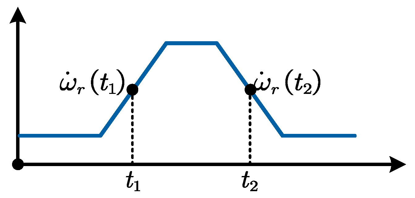
In order to identify the inertia, the coefficient of in Equation (35) should not be zero. Therefore, the IPMSM should be actuated in a speed-varying operation, i.e., . A simple way to conduct the identification process is to force the IPMSM to operate at two different constant accelerations for a short period of time. Meanwhile, the external load torque remains the same.
The speed reference of the LADRC-based drive system is shown in
Figure 9. During the operation, the estimated unknown disturbances at the acceleration moment
and deceleration moment
are stored:
According to the analysis in
Section 4.3, the tracking performance of the LADRC-based speed regulator has a good tolerance for inertia mismatch in low-frequency range. Therefore, the regulator can track the ramp speed reference in
Figure 9 accurately, i.e.,
, and
. Furthermore, the external load torque remains the same during the speed transition, i.e.,
. Moreover, the difference between the unmodeled dynamics
and
can be neglected. Then,
is obtained as:
Finally, the identified inertia is expressed as:
5.2. Improved LADRC-Based Speed Regulator
With the inertia identified, the estimated critical gain
can be automatically adjusted, hence improving the overall performance of the LADRC-based drive system. The block diagram of the improved LADRC-based speed regulator is shown in
Figure 10. In practical applications, the initial inertia
is required. Since the accurate inertia will finally be identified by the proposed method, the initial inertia does not have to be set as accurately as possible. According to the analysis in
Section 4.2, it is suggested that a large
be chosen so as to guarantee the stability of the system.
6. Experimental Results
In this section, experimental results of the proposed LADRC-based IPMSM drive system are presented.
Figure 11 shows the experimental platform. The target machine under test is a three-phase IPMSM, the parameters of which are listed in
Table 1. The IPMSM is driven by a two-level VSI. The control algorithm is implemented on a dSPACE MicroLabBox real-time platform. The dSPACE controller is connected to the VSI through a modulation board. The load torque is provided by an induction machine, which is mechanically coupled with the test machine and controlled by an AC driver. A photoelectric encoder with 2500 threads is utilized to acquire the actual rotor position. The experimental data is transmitted from dSPACE to a desktop computer in digital form through an 100 M ethernet cable. Then, the data is saved to a local directory by ControlDesk (dSPACE GmbH, Paderborn, Germany), the desktop software for dSPACE. Finally, the data is imported to OriginPro software and plotted.
In the following experiments, the sampling and PWM switching frequency are both set to 5 kHz. The deadtime of PWM is set to 1 μs. The DC-link voltage is set to 240 V. The IPMSM is operated in MTPA mode. To reduce the computation burden, the MTPA scheme is implemented by means of look-up tables with offline calculations. The relationship between the torque reference and the
d-
q-axis current references under MPTA operation mode is shown in
Figure 12.
It should be noted that this article mainly concentrates on researching the speed control performance of the LADRC-based drive system. Hence, during the experiments, the parameters for the current loop LADRC are fixed to , . Furthermore, considering the driving capability of the power converter, the torque limit for the speed loop output is set to = 6 N·m.
6.1. Experimental Results of the LADRC-Based IPMSM Drive System with Accurate Inertia
In this experiment, the tracking performance and the disturbance rejection performance of the LADRC-based IPMSM drive system with accurate inertia are evaluated.
Figure 13 shows the experimental results of the speed response with step speed reference from 0 rpm to 1500 rpm. From top to bottom, the plotted signals are
,
, and
. In
Figure 13a, three groups of experiment results with the same
and different
are presented and compared, where
,
. In
Figure 13b, three groups of experiment results with the same
and different
are presented and compared, where
,
. It can be seen that the speed tracking performance is mainly dependent on
. A larger
brings a faster response. It should be noted that since there is a limitation for the speed loop output, the maximum acceleration of speed is restricted. Therefore, the speed response with the step speed reference is actually a ramp response rather than a step response.
Figure 14 shows the experimental results of the speed response with sinusoidal speed reference. The offset, the amplitude, and the frequency of the sinusoidal reference are 1500 rpm, 20 rpm, and 15 Hz, respectively, i.e.,
rpm. From top to bottom, the plotted signals are
,
,
,
, and
. In
Figure 14a, three groups of experiment results with the same
and different
are presented and compared, where
,
. In
Figure 14b, three groups of experiment results with the same
and different
are presented and compared, where
,
. Obviously, the speed tracking performance is mainly dependent on
. A larger
brings a lower tracking latency and a smaller amplitude attenuation.
Figure 15 shows the experimental results of the speed response with step load disturbance. The test IPMSM operates at 1500 rpm. The load IM provides an external step load torque of 3 N·m at 0.3 s. From top to bottom, the plotted signals are
,
,
,
, and
. In
Figure 15a, three groups of experiment results with the same
and different
are presented and compared, where
,
. In
Figure 15b, three groups of experiment results with the same
and different
are presented and compared, where
,
. It can be seen that a larger
or a larger
are both helpful for improving the disturbance rejection performance, and the improvement is relatively more significant when increasing
.
6.2. Experimental Results of the LADRC-Based IPMSM Drive System with Mismatched Inertia
In the following experiment, the tracking performance and the disturbance rejection performance of the LADRC-based IPMSM drive system with mismatched inertia are evaluated.
Figure 16 shows the experimental results of the speed response with step speed reference. Three groups of experiment results with different
are presented and compared, where
,
,
. It can be seen that the speed responses in the three experiments are almost the same. This can be explained according to the analysis in
Figure 5. Since there is a limitation for the speed loop output, the maximum acceleration of speed is restricted. Therefore, the speed response with the step speed reference is actually a ramp response. The ramp speed lies in the low-frequency range in
Figure 5. Therefore, the inertia mismatch has little effect on the speed tracking performance.
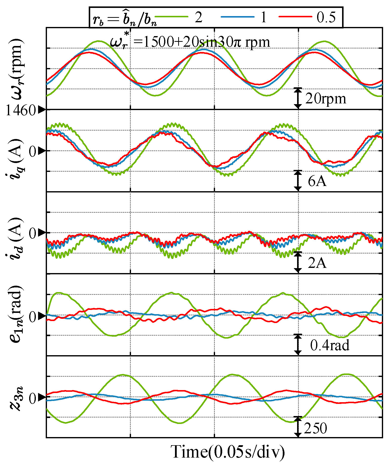
Figure 17 shows the experimental results of the speed response with sinusoidal speed reference. Three groups of experiment results with different
are presented and compared, where
,
,
. It can be seen that
leads to amplitude amplification and phase delay, while
leads to amplitude attenuation and phase advance. This is because the 15 Hz sinusoidal reference lies in the middle-frequency range in
Figure 5. As for the high-frequency range, the corresponding experiments are unable to conduct due to the current limitation of the power converter.
Figure 18 shows the experimental results of the speed response with step load disturbance. Three groups of experiment results with different
are presented and compared, where
,
,
. It can be seen that the speed fluctuation during the loading/unloading process decreases as
decreases, which indicates that the system’s disturbance rejection performance increases as
decreases. These results accord with the analysis in
Figure 6.
6.3. Experimental Results of the Proposed Inertia Identification Method
During this experiment, the IPMSM makes a speed transition from 300 rpm to 1000 rpm, and then back to 300 rpm. The controller parameters are set to
,
.
Figure 19a,b shows the experimental results with initial inertia respectively set to
and
. It can be seen that the identified inertia converges quickly within 0.3 s, and the identified value is close to the actual value, which is 0.0174 kg·m
2.
7. Conclusions
In this article, an improved LADRC scheme for an IPMSM drive system is proposed. The proposed LADRC for speed regulation adopts position feedback instead of speed feedback so that the low-pass filter can be eliminated. Moreover, the MTPA scheme is incorporated into the purposed LADRC to improve the IPMSM drive performance by making full use of its reluctance torque. In addition, considering that the load inertia may vary in some applications, the stability, the tracking performance, and the disturbance rejection performance of the LADRC-based control system with mismatched inertia are analyzed in detail. It is found that the overestimation of inertia can enhance the disturbance rejection performance, but may lead the system to be unstable. As for the tracking performance, it is found that the system will not achieve the desired response as long as the inertia is mismatched. Then, to pursuit a good tracking performance as well as guarantee the system’s stability, an inertia identification method is proposed, which extracts the mismatch information from the estimated disturbance. Extensive experimental results validate the correctness of the theoretical analysis and the effectiveness of the proposed scheme.
However, the designed controller in this article is based an ideal IPMSM model, where the iron losses, the non-sinusoidal back-EMF, the cross-coupling, and the core saturation effect are not considered. In real applications, these unmodelled parts will bring additional disturbance to the drive system and increase the estimation burden of LESO. Thus, the overall performance of the LADRC-based drive system will be degraded. In further research, a more accurate model of IPMSM should be adopted.


