Flywheel Energy Storage System in Italian Regional Transport Railways: A Case Study

Abstract

In this paper, we looked at the role of electromechanical storage in railway applications. A mathematical model of a running train was interfaced with real products on the electromechanical storage market supposed to be installed at the substation. Through this simulation, we gathered data on the recoverable energy of the system, its advantages, and its limitations. Various storage powers were run along variations in speed and gradient to paint a clearer picture of this application. Throughout these simulations, the energy savings were between 25% and 38%, saving up to 0.042 kWh/(seat km).

1. Introduction

Renewable energies are unavoidably subject to variability in accessibility. Wind and sun power, for example, are by their nature unforeseeable and, thus, not programmable [1,2,3]. Today, thanks to technological advances, it is possible to accumulate wind and solar energy and make them available at any time of the day: all thanks to storage and energy accumulation systems. Storage systems are fundamental to the future of sustainable energy [4,5]. Their role is to store electricity and make it available when it is needed most, serving as a balance between supply and demand and helping to stabilize the network [6,7,8,9]. Batteries are today among the most widespread energy storage systems. Year after year, through new research on materials and advanced manufacturing technologies, they are improved, ensuring greater efficiency, low level costs, and a design-to-recycle approach aimed at obtaining an increasingly environmentally sustainable product [10,11,12,13]. One of the most hopeful new technologies for storing and setting the energy grid is the use of flywheel systems, also known as flywheel energy storage systems (FESSs) [14,15]. The system is generally composed of a flywheel, a motor/generator, and the control electronics for connection to an external electrical network. In particular, the system is characterized by the magnetic suspension of the flywheel and its housing in a vacuum chamber. In practice, a flywheel battery absorbs energy from an electrical source in order to charge itself [16,17], stores it in the form of rotational kinetic energy, and when needed, supplies it to the load in the form required by the load itself. The quantity of stored energy depends on the speed of rotation and the inertia of the flywheel, i.e., its size, weight, and the dimension of the rotor radius. There are different types of FESSs, low-speed FESSs characterized by a flywheel rotation speed that can reach 10,000 rpm or high-speed FESSs. These devices operate at extremely high rotational speeds of up to 100,000 rpm. The amount of energy varies from about 5 Wh/kg up to 100 Wh/kg while the efficiency of this system is very high (up to 95%) [18]. The prospective widespread use of the FESSs will be influenced by the progressive reduction of the still very high level of costs, and may also increase due to its flexibility of use; such as in the field of uninterruptible power systems (UPS), for responding to short supply interruptions, or in the transport sector—the latter being analyzed in this article. The energy of a running train is approximately a function of its speed and mass. The regional train of Ferrovie dello Stato, capable of carrying up to 160 seated passengers, weighs approximately 230 tons and cruises at 170 km/h. This yields roughly 71 kWh of energy per train. Most of this energy gets wasted once the train comes to a halt, some of it through friction and some of it through the brakes. This energy could be saved if the latter was stored and re-used at the following departure. Bartlomiejczyk et al. [19] conducted an analysis in Gdynia on the share of energy wasted in a trolleybuses system, reporting potential energy savings of 40%. The power of the E.464, the most common locomotive, is 3.5 MW while its tractive effort is 200 kN [20]. Hillmansen [21] showed that high speeds and short distances between stops increase the efficiency gain through storage. In our simulation, the train runs round-trip the track connecting Genova to La Spezia, stopping at the 30 stations in between. The train runs a track of 86 km, for a cumulative length of 172 km and 63 stations. Studies on energy storage in railway applications [22,23,24,25,26,27,28,29] have been carried out; comparisons with the results found in our studies are examined in Section 4. The altimetric plot is symmetric, i.e., it runs the same path in both ways to eliminate the need to include the potential energy difference between the starting and finishing stations. The storage is hypothesized to be installed at the substation; this has the advantage of being limited by weight and inertial behaviors that occur on board the train, while the disadvantage is the double path the energy has to take, making the whole recovery system less efficient.

2. Mathematical Model

The equations used to model the system are taken from [23]; these were in turn re- adapted from the “modified Davis equation”, “Canadian National Railway formula”, and the formula in use by the French National Railway Company. The free body diagram is composed by three main forces: traction, friction and gradient. The differential equation relating forces and acceleration is the following:

$${\overrightarrow{F}}_{traction}-{\overrightarrow{F}}_{friction}-{\overrightarrow{F}}_{gradient}=M_{train}\cdot \overrightarrow{a}$$

(1)

Since we are dealing with a one-directional problem, the vectorial notation will be omitted. Rochard and Schmid [30] recollected the most common formulae used to calculate train resistances and compared them; the formula used in [23] was chosen for its relatively high values compared to the rest, while the plot below (Figure 1) represents the magnitude of the resistive forces that act on the train at various speeds for the convoy studied. The intersection with the y-axis shows the initial effort the locomotive has to overcome at each starting, while at abscissa greater than zero, the force derived from the plot represents the total resistive forces of the train. The formulae analyzed are: the modified David equation, the French National Railway Company “Société Nationale des Chemins de fer Français” SNCF equation for rolling stock, the SNCF equation for train on bogies, the Strahl equation, and the Sauthoff equation.

2.1. Train and Railway Parameters

The focus of our study is a convoy made up of one E.464 locomotive and four UIC-Z1 carriages. This convoy was chosen because it represents the typical commuter train in Italian railway transport. The data used for this study are reported in (

Table 1. Train and railway parameters.

Name	Description	Unit	Values	Ref.
Mloco	Mass of the locomotive	kg	72,000	[20]
Mcarriage	Mass of the carriage	kg	36,000	-
Mpayload	Mass of the payload (50%)	kg	16,000	-
Ncarriage	Number of carriages	-	4	-
Nloco	Number of locomotives	-	1	-
Naxl	Cumulative number of axles	-	20	-
S	Front surface area	m2	12	-
Ftrain	Maximum traction of locomotive	kN	200	[20]
Ptrain	Maximum power of locomotive	MW	3.5	[20]
Pstorage	Power limit of the FESS	MW	1–1.5–2–2.8	-
ηDC	Substation to wheel efficiency	-	0.8	[23]
ηFW	Flywheel total-total efficiency	-	0.95	[31,32]
pemp	Empirical mass factor	%	8	[23]
$\stackrel{\wedge }{v}$	Maximum speed	m/s	44.5	-
â	Maximum acceleration	m/s2	1.1	[33]
d	Deceleration	m/s2	0.6	[34,35]

) below:

2.2. Drive Cycle

The drive cycle is obtained through an algorithm. The baseline of this algorithm is that the freight accelerates until a point where it either meets the maximum speed or the point at which it needs to start braking. The braking phase is supposed at a constant rate of 0.6 m/s² [34], which is considered a sharp braking. This is done to preserve the comfort of passengers; this value is also found in [35] as 1.5 mph/s (0.67 m/s²). The acceleration is the maximum acceleration allowed by the traction force F_traction as found in [23]. The tractive effort is hence determined as such:

$$F_{traction}=min(F_{train},\frac{P_{train}}{v})$$

(2)

In the figure below, the traction force is represented with respect to velocity. The darker lines represent the ideal forces while the lighter-colored ones represent the forces adjusted by friction (F_traction − F_friction), it also being a function of velocity. The plot (Figure 2) is calculated using a 0% gradient:

Using the tractive effort and the resistive forces obtained above, the acceleration is determined as such:

$$a=\frac{F_{traction}-F_{friction}-F_{gradient}}{M_{train}}$$

(3)

When the instant acceleration is determined, the speed is then updated through the kinematic equation:

$$\frac{dv}{dt}=a v=v_0+{\displaystyle \mathrm{\int }adt}$$

(4)

In the same way, the position is then updated through the equation:

$$\frac{dx}{dt}=a x=x_0+{\displaystyle \int vdt}$$

(5)

It then starts to calculate the braking distance, i.e., the space needed to come to a halt, and compares it to the space between itself and the next station. When the two spaces coincide, the train starts the braking maneuver. After a period of 1 s the algorithm checks the new F_traction, calculates the new acceleration, and the process keeps going until the last station is reached. It is important to note that when F_traction > 0, it represents the pulling force of the motor, while F_traction < 0 represents the braking force. The maximum power transmissible by the locomotive back to the line is equal to its nominal power. The rest of the power needs to either be dissipated through conventional brakes or be sent to the DC line through other generators. If the regenerative braking is only done by the locomotive, it determines the power limit of our storage, after which the locomotive would not be able to supply more power, which in our case is equal to 2.8 MW.

$$P_{lim}^{storage}=P_{train}\cdot {\eta }_{DC}$$

(6)

2.3. Acceleration and Speed Plot

No gradient data is shown below; the effect of the gradient will be discussed in the next chapter. The speed limit in this iteration is set at 31 m/s (110 km/h). The train starts accelerating, tractioned by the maximum effort of the locomotive; once it reaches the power limit, the traction begins to diminish with increasing speeds. It is also possible to observe the traction needed to maintain the constant speed tracts in (Figure 3).

The braking is always constant under the conditions of the simulation; the effect of this approximation will be discussed in a later section. By overlapping the speed and acceleration diagram, we obtain the following graph (Figure 4):

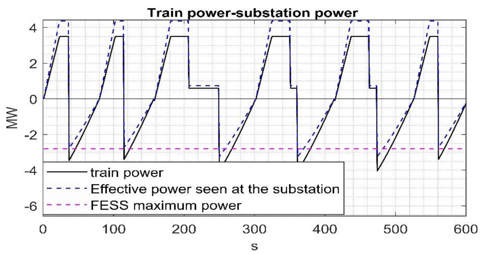
2.4. Energy Management

The storage function is to temporarily hold the train energy while it comes to a halt. In our system, the energy during braking flows from the locomotive (which acts as a generator), through the catenary, to the substation where the storage is hypothesized to be. When the train needs power to accelerate once again, the energy storage gets discharged and power flows again through the catenary, to the locomotive. Train tracks laid in rural areas would be too expensive to retrofit with a catenary, hence why many railway companies adopt diesel locomotives for these tracks. Proposed solutions in [36] include on-board energy storage or short catenaries installed at planned stops to improve efficiency.

3. Energy Estimation and Results

The data crucial to this simulation describe the power consumption during the journey. In the diagram that follows, it is represented in black.

$$P_{traction}=F_{traction}\cdot v$$

(7)

The following graph (Figure 5) also shows P_DC as a blue segmented line, while the purple line represents $P_{lim}^{storage}$, in this case equal to 2.8 MW.

What we are interested in is the energy consumption and the energy recoverable by the FESS. The formula for the energy is as follows:

$$\frac{dE}{dt}=P E=E_0+{\displaystyle \int Pdt}$$

(8)

In the case of the train consumption, P is the power used by the traction forces when P_pos = max(P_traction, 0)

$$E_{pos}^{train}={\displaystyle \int P_{pos}dt}$$

(9)

To understand the limit of our storage, it is also useful to define the total braking energy, i.e., a function of the braking power, the power obtained by the traction forces when P_br = min(P_traction, 0):

$$E_{br}^{train}={\displaystyle \int P_{br}dt}$$

(10)

In the case of the energy stored in the FESS, P_FESS is a function of two variables: the braking power arriving at the substation, $P_{br}^{DC}=P_{br}\cdot {\eta }_{DC}$, and the power limit of the FESS. It can be expressed as follows; it is important to note that the total-to-total efficiency of the flywheel is accounted for in this equation:

$$P_{FESS}=min(\left|P_{br}^{DC}\right|,\left|P^{storage}\right|)$$

(11)

$$E_{FESS}={\displaystyle \int P_{FESS}·{\eta }_{FW}dt}$$

(12)

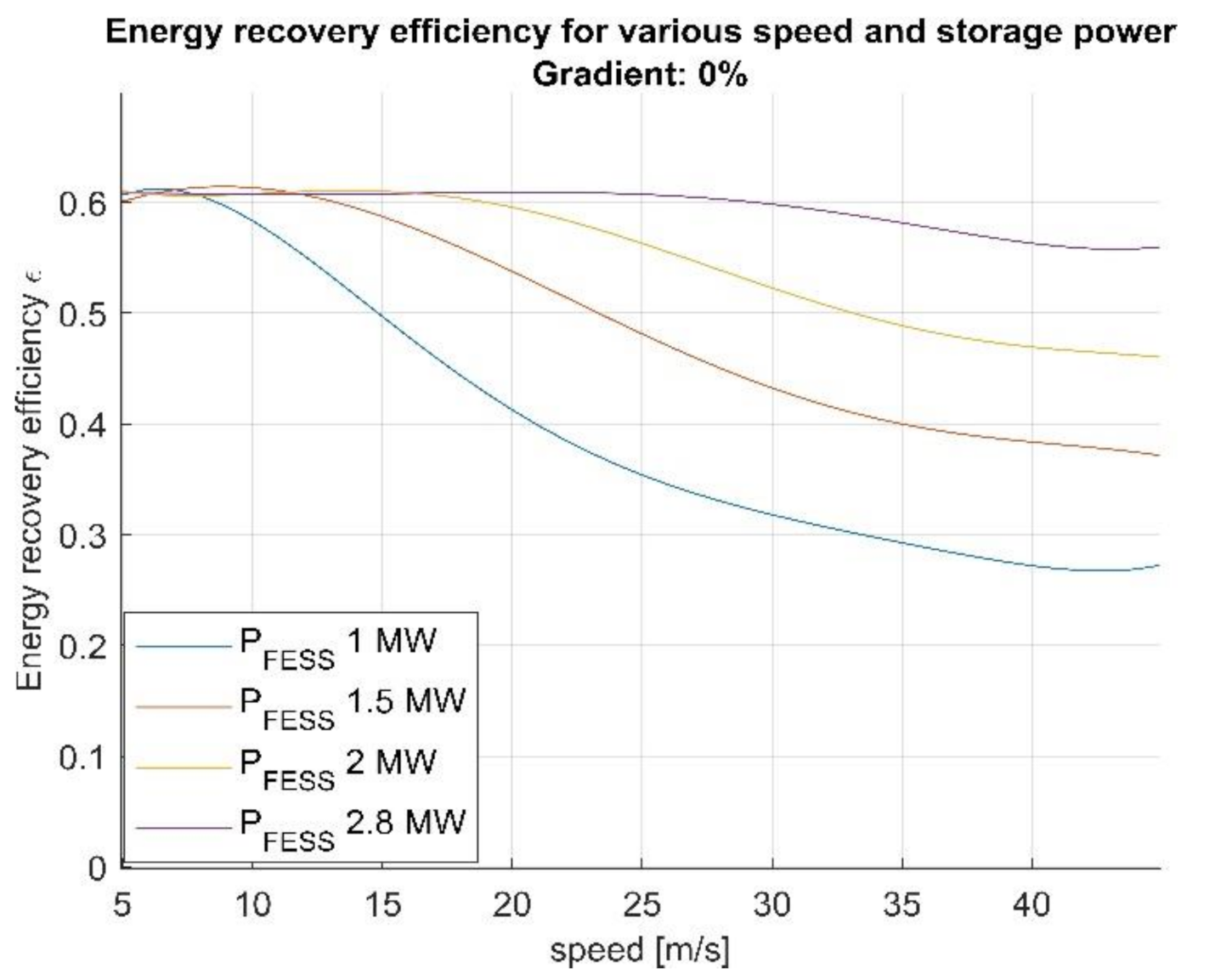
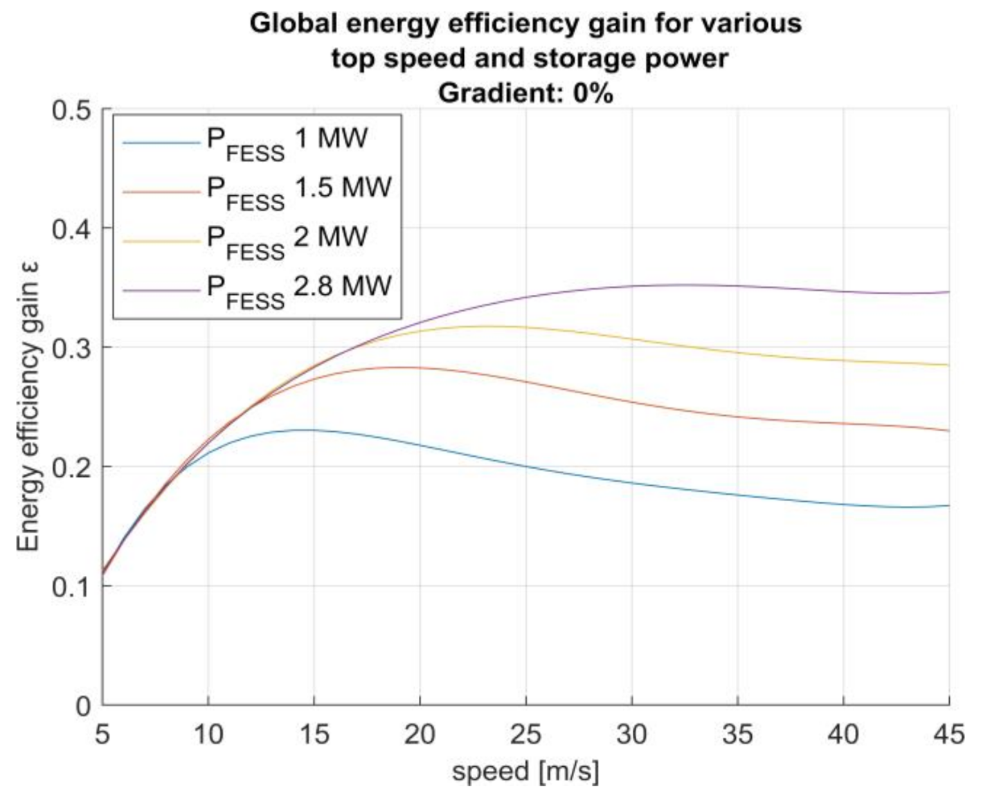
3.1. No Gradient Results

We show below the results of the simulation. According to the results found in [21], higher speeds increase the energy savings; this is due to the fact that losses by friction become proportionally less than the other energies. The simulation estimates the energy required by the train at the substation Equation (13), the braking energy arriving at the substation Equation (14), and the energy gathered by the flywheel Equation (15); the energy recovered is equal to the energy accumulated by the FESS multiplied once again by η_DC due to the fact that the energy has to, once again, flow through the catenary to reach the train. The relations between the energies used are as follows:

$$E_{pos}^{DC}=\frac{E_{pos}^{train}}{{\eta }_{DC}}$$

(13)

$$E_{br}^{DC}=E_{br}^{train}\cdot {\eta }_{DC}$$

(14)

$$E_{recovered}=E_{FESS}\cdot {\eta }_{DC}$$

(15)

It also calculates the efficiency gain 16 as the ratio between the energy recovered and the total energy consumed during the journey, as well as the energy recovery efficiency 17, given by the ratio of the energy recovered and the braking energy:

$$\epsilon =\frac{E_{recovered}}{E_{pos}^{DC}}$$

(16)

$$ϵ=\frac{E_{recovered}}{E_{br}^{train}}$$

(17)

The table below (

Table 2. Results (gradient 0%), P_FESS = $P_{lim}^{storage}$.

Top Speed m/s	${\mathit{E}}_{\mathit{p}\mathit{o}\mathit{s}}^{\mathit{D}\mathit{C}}\left[\mathbf{kWh}\right]$	${\mathit{E}}_{\mathit{b}\mathit{r}}^{\mathit{D}\mathit{C}}\left[\mathbf{kWh}\right]$	EFESS [kWh]	ε	ϵ
12.5	856.5	290.1	275.6	0.257	0.608
18.25	1490	612	581.3	0.312	0.608
25	2308	1043	990.4	0.343	0.608
31.25	3122	1475	1371	0.358	0.605
44.5	4209	2083	1816	0.356	0.557

) recollects the energy drawn at the substation for the entire journey, the braking energy that could arrive at the substation, and the amount of energy that the flywheel could store throughout the journey; it then reports both efficiencies introduced above. As for ε and ϵ, the equations could be re-written using the data available in the table as:

$$\epsilon =\frac{E_{FESS}\cdot {\eta }_{DC}}{E_{pos}^{DC}}$$

(18)

$$ϵ=\frac{E_{FESS}\cdot {\eta }_{DC}^2}{E_{br}^{DC}}$$

(19)

When travelling on an horizontal track, with a top speed of 12.5 m/s, the train consumes 856.5 kWh of energy throughout its journey; of this, 290.1 kWh of energy is dissipated in the braking maneuver. If energy recovery systems were installed, of the 290.1 kWh wasted, 275.1 kWh could be recovered, improving the efficiency of our system by 25.7%. A total of 60.8% of the wasted energy could be recovered, which is the mathematical limit of our model; when the top speed is 44.5 m/s, only 57.5% of the energy could be recovered, while the rest would need to be dissipated or would be lost in the transmission between the train and the substation. In our system there are four main energies: the positive energy, the friction energy, the braking energy, and the energy lost in the transmission, related by the law of conservation of energy:

$$E_{pos}=E_{br}+E_{friction}+E_{losses}$$

(20)

Our recovery system is acting on the braking energy; this is because friction and lost energy are not conservative by definition. As already stated, E_pos can be increased by the multiple stops and high top speed. This way, E_br increases proportionally more than E_friction. The limit to this is given by $P_{lim}^{storage}$, when the speed is too high the power needed to stop is greater than this limit and needs to be disposed in other non-recoverable ways. To overcome this issue, a new braking algorithm could be implemented, such as one limiting the braking power to Pstorage. However, this is beyond the scope of this paper.

The relationships between ϵ (Figure 6), ε (Figure 7), P^storage and $\stackrel{\wedge }{v}$ are the following:

As we can see, there is a speed at which the energy recovery efficiency ϵ starts decreasing. This causes the efficiency gain ε to have a local maximum at speeds that get increasingly higher with Pstorage. For an energy storage power of 1 MW, which represent roughly one third of the power limit of the energy recovery system, the energy recovery efficiency drops from the value of 60.8%, which represents the limit for our storage, to a value of 30% at speed of 40 m/s (144 km/h). Because of this, the efficiency gain at 40 m/s is less than 20%.

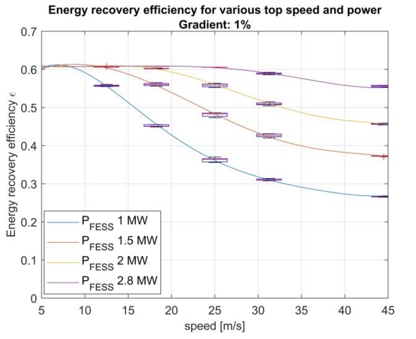
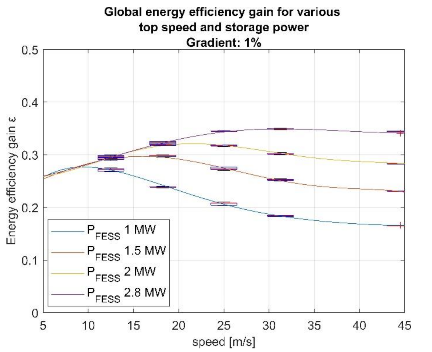
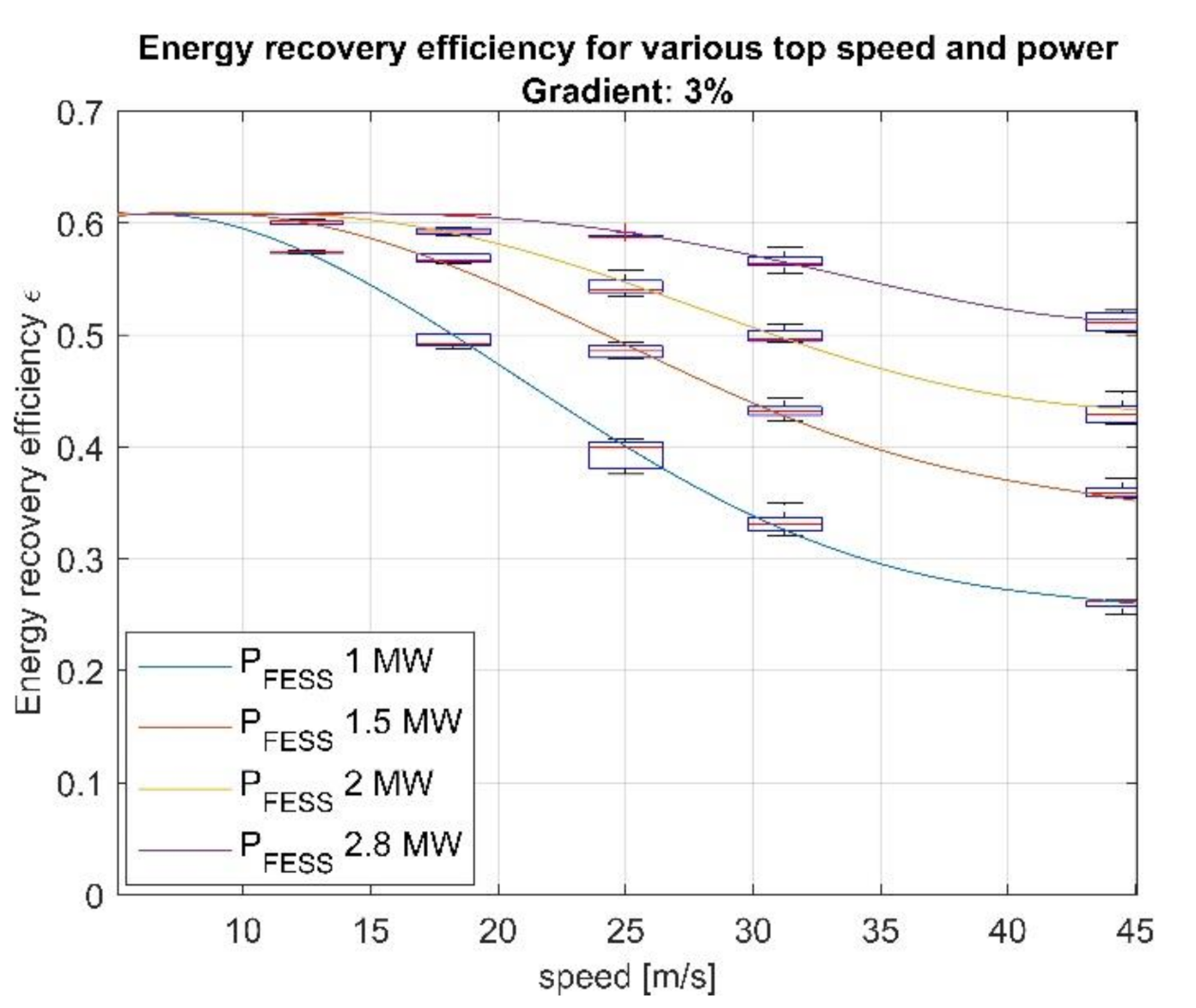
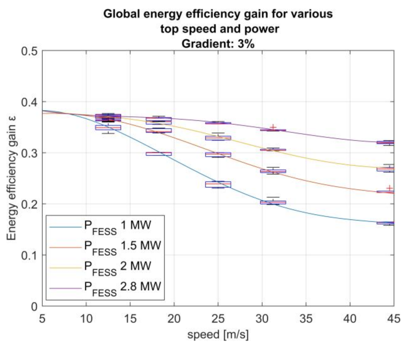
3.2. Gradient Results

The altimetric plot is randomly generated with a slope between the chosen maximum and minimum. In our case, the highest grade analyzed will be 3%. The results given are obtained through various iterations of the simulation and averaged; the standard deviation for the energy recovery efficiency and the efficiency gain has been calculated to be 0.6% for the gradient of 3% and 0.5% for the gradient of 1%. The gradient introduces the conservative gravitational potential energy in the system and consequently the horizontal forces. The effects are twofold and are clearly visible in the equation of conservation of energy:

$$E_{pos}+E{ }_{gravit}^{pos}=E_{friction}+E_{br}+E_{gravit}^{neg}+E_{losses}$$

(21)

At the end of each journey, the magnitude of $E{ }_{gravitational}^{pos}$ and $E{ }_{gravitational}^{neg}$ is always zero. This is because the height difference between the start and finish is null. Throughout the journey, this energy gets accumulated in the train as it rises and is then recovered in the FESS, improving the gain of efficiency of the system. This is because conservative energies constitute a greater share of the total energy. The negative effect occurs during the downhill path: here F_gradient is negative, hence it goes against deceleration. This higher resistance requires more power from the locomotive, which exceeds $P_{lim}^{storage}$ more easily, thus reducing the energy recovery ratio.

The results (

Table 3. Results (gradient 1%), PFESS = $P_{lim}^{storage}$.

Top Speed m/s	${\mathit{E}}_{\mathit{p}\mathit{o}\mathit{s}}^{\mathit{D}\mathit{C}}\left[\mathbf{kWh}\right]$	${\mathit{E}}_{\mathit{b}\mathit{r}}^{\mathit{D}\mathit{C}}\left[\mathbf{kWh}\right]$	EFESS [kWh]	ε	ϵ
12.5	1052	423	401.9	0.305	0.608
18.25	1600	678	644.1	0.322	0.608
25	2381	1088	1028	0.345	0.605
31.25	3131	1475	1371	0.349	0.592
44.5	4230	2097	1799	0.340	0.549

) with a gradient of 1% are represented; for a top speed of 12.5 m/s the total energy consumed for the entire journey is 1052 kWh and the energy dissipated under braking that could be instead reaching the substation is 423 kWh. Of this, 401.9 kWh could be managed to be recovered by the storage when P = $P_{lim}^{storage}$, yielding an efficiency gain of 30.5%. The efficiency gain goes from 30.5% to 34.9%, while the storage efficiency drops from the theoretical limit of 60.8% to 54.9%. The figures regarding the gradient results include a boxplot to represent the distribution of the results obtained through various iterations of the altimetric path. The lines represented represent the average values calculated at each top speed. Below, the results of the effect of P^storage and the top speed are represented for the energy recovery efficiency (Figure 8) and the energy efficiency gain (Figure 9):

This shows that the behavior of the energy recovery ratio ϵ is fairly equal to the no-gradient one. This means that the power generated by the gradient forces is not enough to reach Pstorage sooner than expected, whereas the efficiency gain ε starts at a clearly higher value. Hence, energy recovery systems can start being valuable at lower speeds where a minimal gradient is present.

In this table (

Table 4. Results (gradient 3%), PFESS = $P_{lim}^{storage}$.

Top Speed m/s	${\mathit{E}}_{\mathit{p}\mathit{o}\mathit{s}}^{\mathit{D}\mathit{C}}\left[\mathbf{kWh}\right]$	${\mathit{E}}_{\mathit{b}\mathit{r}}^{\mathit{D}\mathit{C}}\left[\mathbf{kWh}\right]$	EFESS [kWh]	ε	ϵ
12.5	1785	885.7	841.4	0.377	0.608
18.25	2160	1052	995.7	0.369	0.606
25	2785	1320	1223	0.351	0.593
31.25	3359	1611	1438	0.342	0.571
44.5	4445	2219	1743	0.314	0.503

), the numerical results for a gradient of 3% are represented; for a top speed of 12.5 m/s, the total energy consumed for the entire journey is 1785 kWh and the energy dissipated under braking that could be instead reaching the substation is 885.7 kWh. Of this, 841.4 kWh could be managed to be recovered by the storage when P = $P_{lim}^{storage}$, yielding an energy recovery ratio of 37.7%. When the top speed is set at 44.5 m/s, the energy consumed is equal to 4445 kWh, while the efficiency gain is 31.4%. The energy recovery ratio, i.e., the braking energy that the system manages to recover, is 50.3%; this is dictated by the high top speed and the high bursts of power needed to slow down the convoy. Below, the effects of the storage size and top speed are plotted for the energy recovery efficiency (Figure 10) and the energy efficiency gain (Figure 11):

When the gradient is 3%, its effects on ϵ start to become more visible. The value starts at 37.7% and drops off to 31.4% at 44.5 m/s (160 km/h) where Pstorage = 2.8 MW. Where Pstorage = 1 MW, its value is 16%. The efficiency of the energy saving is much more prominent at low speed with a steep gradient, while its effects at higher speed start diminishing. The energy recovery efficiency could be improved, as already stated, by a different braking algorithm.

3.3. Energy Savings

The mathematical model implemented outputted results of various iterations where geography, top speed, and type of storage were changed. This showed the potential energy savings. A way to express savings is by the energy consumed and saved per seat per kilometer; [37] reports values between 0.05 [$\frac{kWh}{seat\cdot km}$] to 0.09 [$\frac{kWh}{seat\cdot km}$], while according to our studies, the results are the following. It is important to note the generality of the results reported in the aforementioned study when comparing them to our results reported in (

Table 5. Energy per seat per kilometer. Top speed 18.25 m/s.

Gradient	$\mathbf{Consumed} \left[\frac{\mathbf{k}\mathbf{W}\mathbf{h}}{\mathbf{s}\mathbf{e}\mathbf{a}\mathbf{t}\cdot \mathbf{k}\mathbf{m}}\right]$	$\mathbf{Saved} \left[\frac{\mathbf{k}\mathbf{W}\mathbf{h}}{\mathbf{s}\mathbf{e}\mathbf{a}\mathbf{t}\cdot \mathbf{k}\mathbf{m}}\right]$
0%	0.054	0.017
1%	0.058	0.019
3%	0.078	0.029

) and (

Table 6. Energy per seat per kilometer. Top speed 31.25 m/s.

Gradient	$\mathbf{Consumed} \left[\frac{\mathbf{k}\mathbf{W}\mathbf{h}}{\mathbf{s}\mathbf{e}\mathbf{a}\mathbf{t}\cdot \mathbf{k}\mathbf{m}}\right]$	$\mathbf{Saved} \left[\frac{\mathbf{k}\mathbf{W}\mathbf{h}}{\mathbf{s}\mathbf{e}\mathbf{a}\mathbf{t}\cdot \mathbf{k}\mathbf{m}}\right]$
0%	0.112	0.041
1%	0.112	0.040
3%	0.122	0.042

).

It is therefore possible to conclude that quayside storage, with a nominal power adjusted by efficiency and equal to that of the locomotive, can improve the efficiency of our modeled railway from 25% to 38%, despite the disadvantageous path the energy has to make. Comparatively, energy storage with a peak power of one third of that of the locomotive can improve the efficiency by more than 15%.

4. Discussion

A comprehensive study reviewed state-of-the-art technologies for energy recovery systems in railway systems [38] and reported real-world results of energy savings between 20% and 30%. As for on-board energy storage, savings are reported at 24% [39] and 18.6–35.6% [40]. These values refer to real-world data and account for phenomena that cannot be properly modelled. Applications of FESS in railways in New York, according to one study [22], have been adopted since 2000. This demonstrates that energy storage can reduce the peak power demands at the rectifier and provide reinforcement to the supply infrastructure; it can also provide additional energy savings with regenerative motors on-board the train. As already pointed out by Rupp et al. [23], the literature on FESS storage in railway application is somewhat limited. According to their study, the savings were between 9.83% to 31.21%. The focus of their study was a light transit convoy with on-board FESS. Under their hypothesis, the track had no gradient. Due to inherent differences in the convoy Rupp et al. studied and our own convoy model, our data for no-gradient conditions reports efficiencies between 16.7% and 35.6% depending on the storage nominal power. Barrero et al. [27] modelled a metro network with stationary and on-board Energy Storage Systems (ESS) and found that reduction achieved with stationary ESS varies as a function of the traffic conditions, ESS size, and ESS distribution along the line. With efficient metro trains, savings were 18.7%, 25.1%, and 36.4% at high, moderate, and low traffic volumes, respectively. Whereas, using on-board ESS on every vehicle, the maximum energy savings achieved varied between 27.3% and 36.3% at high and low traffic volumes, respectively. The results reported by Barrero et al. for low traffic volume match quite well with our findings; this is because the track we analyzed was run by only a single train. This underlines the importance of studying the interaction of multiple trains on the same line, which will be one of the focuses of our next studies. Li et al. [28] introduced a prototype FESS for commuter trains, though their focus was on the manufacturing processes for the FESS. Hillmansen and Roberts analyzed a high-speed and a commuter diesel train combined with energy storage in [29] and found savings of 28% and 35% respectively, while the energy per seat per kilometer travelled saved was 0.02 kWh/(seat km). The results of the energy efficiency gain are in accordance with our results, while the energy saved per seat per kilometer depends on the convoy chosen, its top speed, and the layout of the track. Chymera et al. showed that more than 50% of the energy dissipated in a transit system comes from braking [30], which also sets a limit on the energy that can be recovered through energy storage. The authors of [40] conduct a similar study to ours on a Brazilian route, calculating a theoretical 23.87% energy savings; when introducing the optimal size storage, an energy savings of 15.67% is achieved. [31] shows how coupling a flywheel in a slug car can reduce fuel consumption and NOx emissions by recovering the braking energy; gas emission reduction is another factor to take into account when dealing with ICE locomotives. Given the energy savings sourced in these aforementioned publications and the ones calculated in our studies, it is possible to conclude that our model is behaving as expected, yielding results for various configurations and showing, for each case, the expected energy savings for our case. It is important to conclude that the energy savings percentage is not the only figure to observe: costs and total energy consumed are an important factor to include in designing new railways or retrofitting ESS into existing ones.

5. Conclusions

Along with the number of stops and top speed [21], it is also possible to conclude that the gradient of the track plays a great role in low top speed systems, where the effort to overcome the steepness of the grade is comparable to that needed to overcome the friction and resistance of the train. This underlines the beneficial efficiency gains of installing storage facilities on tracks with a relevant altimetric gain with respect to flat tracks. In any case, the results have hereby been proven to be applicable to any track and for any reasonable nominal power. The economical matter is being worked on by the authors, who will try to find the optimal size for storage and energy capacity in a given system. Further studies on braking algorithms and their effect on travel time and gained efficiency alongside the storage energy capacity are encouraged and will be a focus of our next studies. Even though these results were obtained for a single train and a single route, this study can be adapted for various cases and is advised for any future railway planning. A railway system will also be modeled to study the interactions between multiple rolling stocks of different kinds.

References

1. Khare, V.; Nema, S.; Baredar, P. Solar-wind Hybrid Renewable Energy System: A Review. Renew. Sustain. Energy Rev. 2016, 58, 23–33. [Google Scholar] [CrossRef]
2. Elhadidy, M.A.; Shaahid, S.M. Parametric Study of Hybrid (Wind Solar Diesel) Power Generating Systems. Renew. Energy 2000, 21, 129–139. [Google Scholar] [CrossRef]
3. Lior, N. Sustainable Energy Development: The Present (2009) Situation and Possible Paths to the Future. Energy 2010, 35, 3976–3994. [Google Scholar] [CrossRef]
4. Ibrahim, H.; Ilinca, A.; Perron, J. Energy Storage Systems—Characteristics and Comparisons. Renew. Sustain. Energy Rev. 2008, 12, 1221–1250. [Google Scholar] [CrossRef]
5. Ebrahim, T.; Zhang, B. CleanTX Analysis on Energy Storage; Cleanenergy Incubator, University of Texas at Austin: Austin, TX, USA, 2008. [Google Scholar]
6. Palizban, O.; Kauhaniemi, K. Energy Storage Systems in Modern Grids—Matrix of Technologies and Applications. J. Energy Storage 2016, 6, 248–259. [Google Scholar] [CrossRef]
7. U.S. Department of Energy. Grid Energy Storage; U.S. Department of Energy: Washington, DC, USA, 2013.
8. Strzelecki, R.M.; Benysek, G. (Eds.) Power Electronics in Smart Electrical Energy Networks; Springer Science & Business Media: Berlin/Heidelberg, Germany, 2008. [Google Scholar]
9. Zhao, H.; Wu, Q.; Hu, S.; Xu, H.; Rasmussen, C.N. Review of Energy Storage System for Wind Power Integration Support. Appl. Energy 2015, 137, 545–553. [Google Scholar] [CrossRef]
10. Reihani, E.; Sepasi, S.; Roose, L.R.; Matsuura, M. Energy Management at the Distribution Grid Using a Battery Energy Storage System (BESS). Int. J. Electr. Power Energy Syst. 2016, 77, 337–344. [Google Scholar] [CrossRef]
11. Oudalov, A.; Cherkaoui, R.; Beguin, A. Sizing and optimal operation of battery energy storage system for peak shaving application. In Proceedings of the 2007 IEEE Lausanne Power Tech, Lausanne, Switzerland, 1–5 July 2007. [Google Scholar]
12. Riffonneau, Y.; Bacha, S.; Barruel, F.; Ploix, S. Optimal power flow management for grid connected PV systems with batteries. IEEE Trans. Sustain. Energy 2011, 2, 309–320. [Google Scholar] [CrossRef]
13. Mehr, T.H.; Masoum, M.A.; Jabalameli, N. Grid-connected lithium-ion battery energy storage system for load leveling and peak shaving. In Proceedings of the 2013 Australasian Universities Power Engineering Conference (AUPEC), Hobart, Australia, 29 September–3 October 2013. [Google Scholar]
14. Lee, H.; Shin, B.Y.; Han, S.; Jung, S.; Park, B.; Jang, G. Compensation for the power fluctuation of the large scale wind farm using hybrid energy storage applications. IEEE Trans. Appl. Supercond. 2011, 22, 5701904. [Google Scholar]
15. Kailasan, A.; Dimond, T.; Allaire, P.; Sheffler, D. Design and Analysis of a Unique Energy Storage Flywheel System—An Integrated Flywheel, Motor/Generator, and Magnetic Bearing Configuration. ASME J. Eng. Gas Turbines Power 2015, 137, 042505. [Google Scholar] [CrossRef]
16. Liu, H.; Jiang, J. Flywheel Energy Storage—An Upswing Technology for Energy Sustainability. Energy Build. 2007, 39, 599–604. [Google Scholar] [CrossRef]
17. Genta, G. Kinetic Energy Storage Theory and Practice of Advanced Flywheel Systems; Butterworths: London, UK, 1985. [Google Scholar]
18. Ahrens, M.; Kucera, L.; Larsonneur, R. Performance of a Magnetically Suspended Flywheel Energy Storage Device. IEEE Trans. Control Syst. Technol. 1996, 4, 494–502. [Google Scholar] [CrossRef]
19. Bartłomiejczyk, M.; Połom, M. Multiaspect Measurement Analysis of Breaking Energy Recovery. Energy Convers. Manag. 2016, 127, 35–42. [Google Scholar] [CrossRef]
20. Ferrovie Emilia Romagna, Immatricolazione E.464. 2009. Available online: https://www.fer.it/wp-content/uploads/2015/04/CIG-5004756C58-Allegato-1-al-Capitolato_documentazione-tecnica.pdf (accessed on 10 October 2021). (In Italian).
21. Hillmansen, S. Sustainable Traction Drives. In Proceedings of the 7th IET Professional Development Course on Railway Electrification Infrastructure and Systems (REIS 2015), London, UK, 8–11 June 2015; p. 15. [Google Scholar] [CrossRef]
22. Richardson, M.B. Flywheel Energy Storage System for Traction Applications. In Proceedings of the International Conference on Power Electronics Machines and Drives, Sante Fe, NM, USA, 4–7 June 2002; pp. 275–279. [Google Scholar] [CrossRef]
23. Rupp, A.; Baier, H.; Mertiny, P.; Secanell, M. Analysis of a Flywheel Energy Storage System for Light Rail Transit. Energy 2016, 107, 625–638. [Google Scholar] [CrossRef]
24. Barrero, R.; Tackoen, X.; Van Mierlo, J. Stationary or Onboard Energy Storage Systems for Energy Consumption Reduction in a Metro Network. Proc. Inst. Mech. Eng. F J. Rail Rapid Transit 2010, 224, 207–225. [Google Scholar] [CrossRef]
25. Li, Y.L.; Zhang, X.Z.; Dai, X.J. Flywheel Energy Storage System for City Trains to Save Energy. Adv. Mater. Res. 2012, 512–515, 1045–1048. [Google Scholar] [CrossRef]
26. Hillmansen, S.; Roberts, C. Energy Storage Devices in Hybrid Railway Vehicles: A Kinematic Analysis. Proc. Inst. Mech. Eng. F J. Rail Rapid Transit 2007, 221, 135–143. [Google Scholar] [CrossRef]
27. Renfrew, A.C.; Chymera, M.; Barnes, M. Analysis of Energy Dissipation in an Electric Transit System. In Proceedings of the IEEE/ASME/ASCE 2008 Joint Rail Conference, Wilmington, DE, USA, 22–24 April 2008; pp. 321–326. [Google Scholar] [CrossRef]
28. Wang, Z.; Palazzolo, A.; Park, J. Hybrid Train Power with Diesel Locomotive and Slug Car–Based Flywheels for NOx and Fuel Reduction. J. Energy Eng. 2012, 138, 215–236. [Google Scholar] [CrossRef] [Green Version]
29. Frilli, A.; Meli, E.; Nocciolini, D.; Pugi, L.; Rindi, A. Energetic Optimization of Regenerative Braking for High Speed Railway Systems. Energy Convers. Manag. 2016, 129, 200–215. [Google Scholar] [CrossRef]
30. Rochard, B.P.; Schmid, F. A Review of Methods to Measure and Calculate Train Resistances. Proc. Inst. Mech. Eng. F J. Rail Rapid Transit 2000, 214, 185–199. [Google Scholar] [CrossRef]
31. Piller Power Systems. Piller UB-V Series. 2021. Online Datasheet. Available online: https://www.piller.com/en-GB/2777/critical-power-modules-cpm-with-flywheel (accessed on 10 September 2021).
32. Sabihuddin, S.; Kiprakis, A.E.; Mueller, M. A Numerical and Graphical Review of Energy Storage Technologies. Energies 2015, 8, 172–216. [Google Scholar] [CrossRef]
33. Bae, I.; Moon, J.; Seo, J. Toward a Comfortable Driving Experience for a Self-driving Shuttle Bus. Electronics 2019, 8, 943. [Google Scholar] [CrossRef] [Green Version]
34. Quaglietta, E. A Microscopic Simulation Model for Supporting the Design of Railway Systems: Development and Applications. Ph.D. Thesis, University of Naples Federico II, Naples, Italy, 2011. [Google Scholar]
35. Francis, H.; Dressel, D.E. Electric Railway Engineering; Franklin Classics Trade Press: New York, NY, USA, 2018. [Google Scholar]
36. Mayrink, S., Jr.; Oliveira, J.G.; Dias, B.H.; Oliveira, L.W.; Ochoa, J.S.; Rosseti, G.S. Regenerative Braking for Energy Recovering in Diesel-Electric Freight Trains: A Technical and Economic Evaluation. Energies 2020, 13, 963. [Google Scholar] [CrossRef] [Green Version]
37. Perez-Martinez, P.J.; Ivan, A.S. Energy consumption of passenger land transport modes. Energy Environ. 2010, 21, 577–600. [Google Scholar] [CrossRef]
38. Khodaparastan, M.; Mohamed, A.A.; Brandauer, W. Recuperation of Regenerative Braking Energy in Electric Rail Transit Systems. IEEE Trans. Intell. Transp. Syst. 2019, 20, 2831–2847. [Google Scholar] [CrossRef] [Green Version]
39. Domínguez, M.; Cucala, A.; Fernández, A.; Pecharromán, R.; Blanquer, J. Energy efficiency on train control: Design of metro ATO driving and impact of energy accumulation devices. In Proceedings of the 9th World Congress on Railway Research, Lille, France, 22–26 May 2011. [Google Scholar]
40. Barrero, R.; Van Mierlo, J.; Tackoen, X. Energy Savings in Public Transport. IEEE Veh. Technol. Mag. 2008, 3, 26–36. [Google Scholar] [CrossRef]
Figure 1. Train friction forces obtained through different formulae.
Energies 15 01096 g001
Figure 2. Tractive effort of the locomotive.
Energies 15 01096 g002
Figure 3. Locomotive forces in the first 600 s.
Energies 15 01096 g003
Figure 4. Speed and acceleration plot over time.
Energies 15 01096 g004
Figure 5. Train power and substation power during the journey.
Energies 15 01096 g005
Figure 6. No gradient energy recovery efficiency for multiple top speeds and FESS powers.
Energies 15 01096 g006
Figure 7. No gradient efficiency gain for multiple top speeds and FESS powers.
Energies 15 01096 g007
Figure 8. One percent gradient energy recovery efficiency for multiple top speeds and FESS powers.
Energies 15 01096 g008
Figure 9. One percent gradient efficiency gain for multiple top speeds and FESS powers.
Energies 15 01096 g009
Figure 10. Three percent gradient energy recovery efficiency for multiple top speeds and FESS powers.
Energies 15 01096 g010
Figure 11. Three percent gradient efficiency gain for multiple top speeds and FESS powers.
Energies 15 01096 g011