Article

A Grid-Connected Microgrid Model and Optimal Scheduling Strategy Based on Hybrid Energy Storage System and Demand-Side Response

1
School of Management, Guizhou University, Guiyang 550025, China
2
Key Laboratory of “Internet+” Collaborative Intelligent Manufacturing in Guizhou Province, Guiyang 550025, China
*
Author to whom correspondence should be addressed.
Energies 2022, 15(3), 1060; https://doi.org/10.3390/en15031060
Submission received: 30 November 2021 / Revised: 2 January 2022 / Accepted: 24 January 2022 / Published: 31 January 2022

Abstract

:
The power gap between supply and demand in the microgrid caused by the uncertainty of wind and solar output and users’ electricity consumption needs to be absorbed by the hybrid energy storage devices and the demand-side electricity price response. To maximize the service life of the lithium battery pack, this paper optimizes a reasonable ratio of the supercapacitor pack’s daily charge and discharge times to the daily cycle times of the lithium battery pack. The model construction includes two parts: power prediction and multi-objective optimization modeling. In the case study, a microgrid district under the Guizhou Power Grid is analyzed and discussed. Based on the predicted wind output, solar output, and load demand on a certain day, the optimal scheduling results have been obtained. On the one hand, a reasonable ratio regarding the daily charge and discharge times of hybrid energy storage devices has been obtained under the optimized parameter k in the model. Correspondingly, the daily operation and maintenance of the lithium battery pack is minimum. On the other hand, when the hybrid energy storage devices and demand-side electricity price response are included and not, the changes on the supply and demand sides (a) and of three evaluation indicators (b) are compared, respectively. Thus, the effectiveness of the model in this paper is verified.

1. Introduction

The microgrid is a small power grid composed of the distributed power supply, the energy storage device, the load, etc. [1]. The connection of wind and solar renewable energy into the distribution network (DN) in the form of the microgrid is generally considered to be an effective method to absorb renewable energy nearby. However, the scale of the microgrid is small and its self-regulation ability is weak. The active power balance and voltage stability [1] of it is therefore extremely susceptible to the intermittency and fluctuation of wind and solar output power and the randomness of electricity consumption of users, posing an urgent problem to be solved for the operation of the microgrid. The energy storage device is designed to reduce the uncertainty of supply and demand. The hybrid energy storage devices composed of the supercapacitor pack and the lithium battery pack can make up for the technical defect of a single energy storage device and achieve complementary advantages [2,3]. The uncertainty on both sides of the supply and demand would cause the supply and demand power gap. The power gap would be allocated between the supercapacitor pack and the lithium battery pack. In the allocation what should be paid attention to is the reasonable ratio of the daily charge and discharge times of the supercapacitor pack to the daily cycle times of the lithium battery pack. If the ratio is unreasonable, the service life of the lithium battery pack will be affected. As a result, it is necessary to optimize and decide the aforementioned “reasonable ratio”.
As far as the absorption of the power gap between supply and demand is concerned, previous research mostly focused on the descriptive methods of the uncertainty of the renewable energy output, such as the scene method [4,5]. References [6,7,8,9] only include the battery energy storage device. Reference [10] deals with the intermittency and volatility of the renewable energy output power directly from the perspective of supply and demand collaborative scheduling, yet does not focus on hybrid energy storage devices’ charging and discharging process when they are applied to solve this problem. As far as the problem of maximizing the service life of the battery equipment is concerned, the previous literature [11,12,13] that used hybrid energy storage devices to absorb the power gap rarely considered maximizing the service life of the battery equipment simultaneously. References [3,8,14] do not consider the goal of maximizing the service life of a battery device. Among them, Reference [8] believes that the purpose of prolonging the service life of the battery equipment could be achieved by bringing in the state-of-charge (SOC) constraint and the charge and discharge power constraint of battery equipment. These two constraints are only general constraints of battery equipment. Previous studies that consider the problem of maximizing the service life of the battery equipment focus on the total operation cost of energy storage [15,16,17,18,19,20], SOC [21], the charge and discharge power [10], and the life model [22,23,24]. These angles lack practicality for they are either not that convincing or the model is complex. For example, in Reference [15], the battery’s service life is reflected on the parameters of the investment cost and operation and maintenance cost, namely the theoretical cycle times and the operation and maintenance cost coefficients. Compared with obtaining the battery’s cycle times by optimization, these parameters are constant. From the perspective of minimizing the daily cycle times of the battery to maximize the battery’s service life, its method is not that convincing in the effect of achieving the battery’s service life maximization. By contrast, to represent the service life of the battery equipment by cycle times is both theoretically based and easy to understand. Maximizing the service life of the battery equipment can be interpreted as that the battery equipment can be used for more years. Since the service life is the ratio of the theoretical cycle times to the annual cycle times [25], it is necessary to minimize the daily cycles times of the battery equipment. In addition to dispatching the hybrid energy storage devices, the absorption of the power gap between supply and demand can also rely on the demand side electricity price response [4,26,27]. The elastic load is a kind of load that can be adjusted flexibly by the microgrid operator according to the supply conditions. According to the characteristic of the elastic load being sensitive to the change of the electricity price [28], the microgrid operator can formulate the demand-side electricity price response function used to (1) guide the elastic load consumers to adjust their habits of electricity consumption, (2) reduce the peak and valley difference of the load curve [29], and (3) reduce the electricity purchased from the distribution network.
For the absorption of the power gap between supply and demand, on the one hand, dispatch the hybrid energy storage devices from the supply-side perspective. To maximize the service life of the lithium battery pack, this article makes an optimization decision on the reasonable ratio of the supercapacitor pack’s daily charge and discharge times to the lithium battery pack’s daily cycle times; on the other hand, consider the demand-side electricity price response from the demand-side perspective. This paper makes an optimization decision on the elastic load transfer power. Academic contribution is to make the ratio of the power type supercapacitor pack’s daily charge and discharge times to the energy type lithium battery pack’s daily cycle times as reasonable as possible to maximize the service life of the lithium battery pack and reduce its operation and maintenance cost.
This paper is organized as follows: Section 2 is an overview of the microgrid system; Section 3 introduces the methodology; Section 4 gives and discusses the optimal scheduling results; Section 5 summarizes the outcome of the paper.

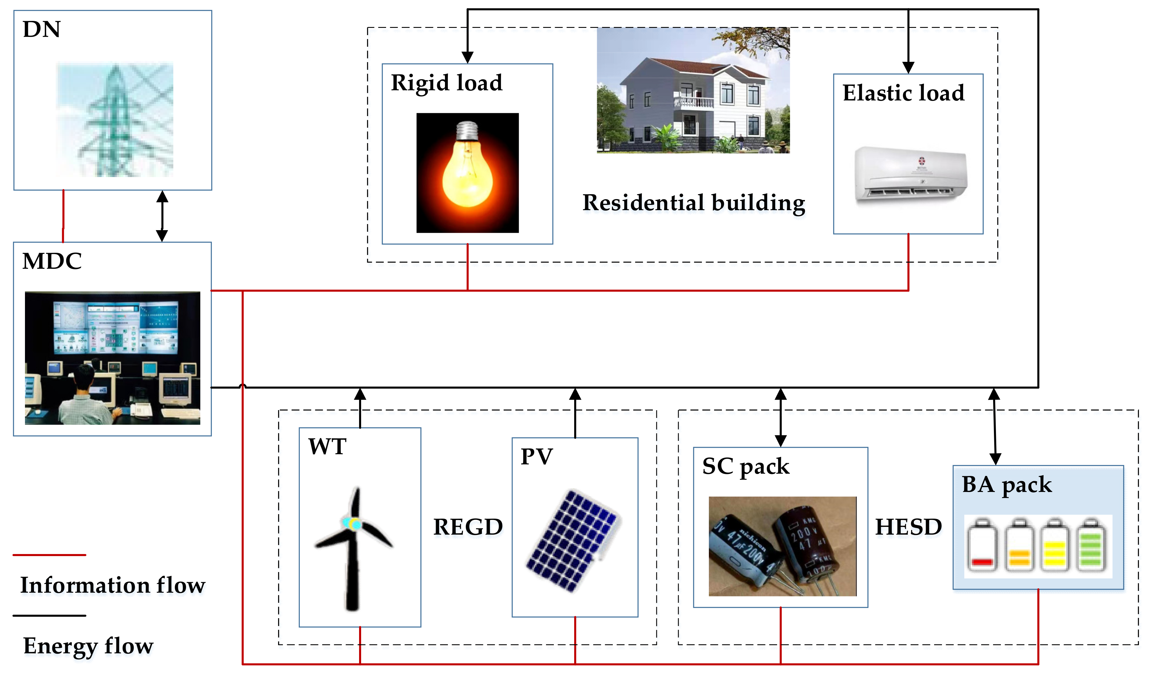
2. Overview of the Microgrid System

An enormous number of microgrids exist throughout western China. As a kind of distributed power source, these microgrids play important roles in terms of people’s daily life. Among them, Guizhou Province, located on the Yunnan-Guizhou Plateau in southwest China, is relatively rich in wind energy resources. Moreover, the scale of photovoltaic power generation projects in western Guizhou has developed rapidly in recent years. Therefore, a microgrid system can be built according to local conditions [30], and clean energy can be used to solve local energy demand problems, which is conducive to improving the level of regional renewable energy utilization and promoting regional economic development. When the distributed power generation in the grid is insufficient, the microgrid is connected to the distribution network to ensure a continuous power supply. Under the jurisdiction of a distribution network (e.g., the Guizhou Power Grid) are a host of microgrids. This article takes one of them as an example. The basic framework of a microgrid district under the Guizhou Power Grid is shown in Figure 1.
The microgrid district consists of renewable energy generation devices (REGD), hybrid energy storage devices (HESD), the load, and a microgrid dispatch center (MDC). (1) Renewable energy generation devices include wind turbines (WT) and photovoltaic (PV), whose output power is intermittent and uncertain due to climate conditions. (2) Hybrid energy storage devices include a supercapacitor pack (SC pack) and a lithium battery pack (BA pack), which are used to alleviate the intermittency and uncertainty of the renewable energy output power and the randomness of users’ electricity consumption. When the total wind and solar output power is higher than the load, the hybrid energy storage devices are charged, and vice versa. (3) The load is divided into rigid load and elastic load. The microgrid operator can adjust the elastic load by means of electricity price to achieve the lowest power supply cost while ensuring that the user satisfaction with electricity will not be significantly reduced. (4) Renewable energy generation devices, hybrid energy storage devices, and the load are connected to the microgrid dispatching center through the communication network. The microgrid dispatching center obtains the real-time power supply and load demand information and adjusts these devices according to the energy optimization dispatching strategy.
However, due to the small scale of the microgrid district and its weak self-regulation ability, to meet the instantaneous balance of power, it is necessary to accurately predict the power generation and the load of a certain day in the future. To overcome the intermittency of wind and solar output power, it is necessary to equip the hybrid energy storage devices to charge when the supply exceeds demand, and vice versa. But lithium batteries are not only expensive but also have far fewer cycle times than supercapacitors. Therefore, it is necessary to decide a reasonable ratio of the charge and discharge times of supercapacitors to the cycle times of lithium batteries to maximize the service life of the lithium battery pack. Significantly, whether electricity is purchased or sold, grid connection is the last choice of the microgrid. In other words, when the supply is less than the demand, it will not be considered to purchase electricity from the distribution network until all the power sources in the microgrid are put into use but still cannot meet the demand; When the supply exceeds the demand, it will not be considered to sell electricity to the distribution network until all the loads in the microgrid are satisfied but there is remaining wind and solar output power.

3. Methodology

This paper adopts the Back Propagation (BP) neural network to predict the power generation and the load of a certain day in the future, and also sets up the multi-objective model to make the ratio of the supercapacitor pack’s daily charge and discharge times to the lithium battery pack’s daily cycle times as reasonable as possible.

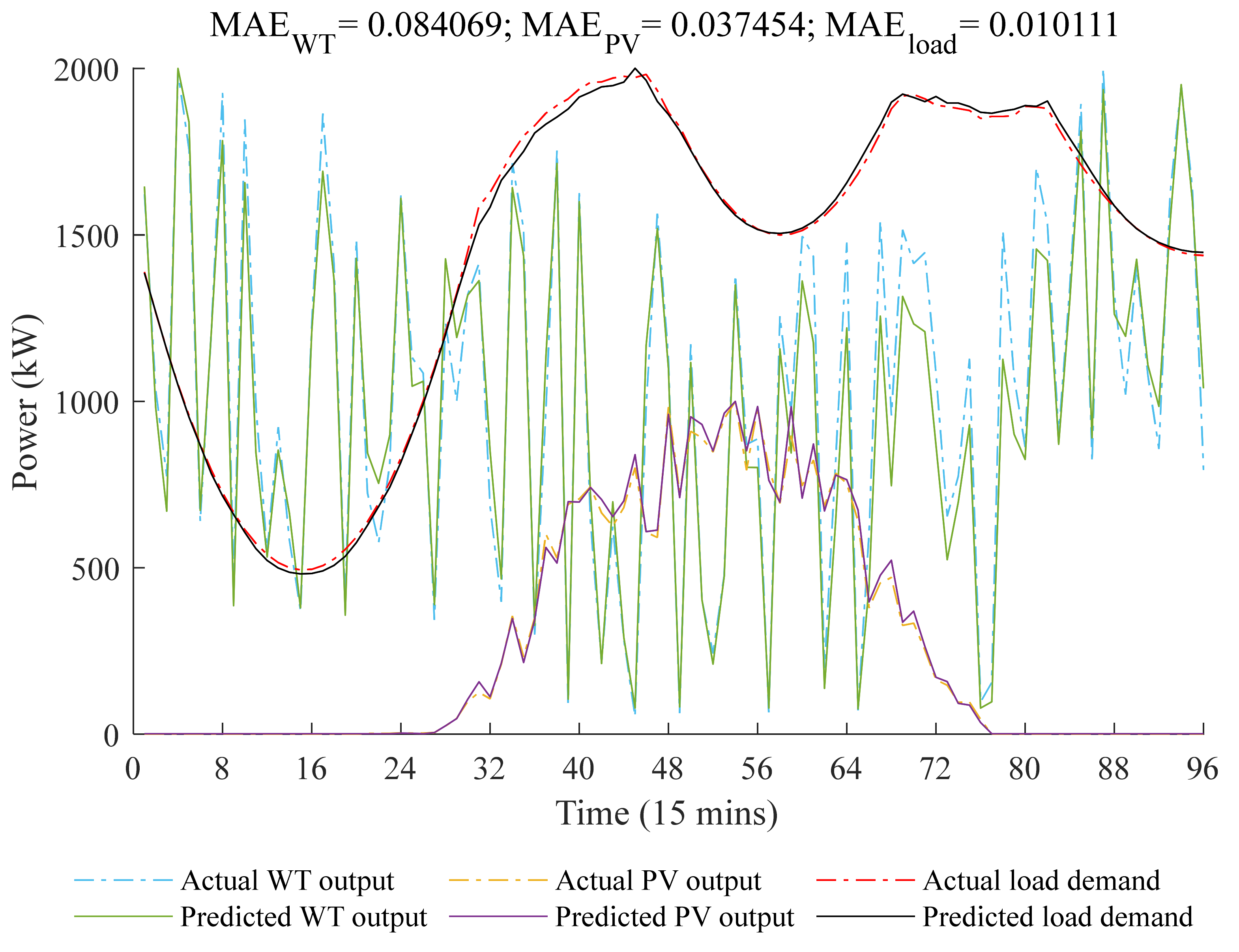
3.1. Power Prediction

This paper uses the BP neural network to predict the wind power, photovoltaic power, and total load power of the summer typical day in the next year of the microgrid community. The input values of the BP neural network are set as the various power of the summer typical day in the previous two years of the district. The output values of the BP neural network are set as the various power of the summer typical day in the third year of the district. The error evaluation indices of the test set are the mean absolute error (MAE) (see Equation (1)) and the difference calculation of the F test (use the Excel software to get the difference calculation table of the F test).
MAE = 1 N s a m = 1 N s a X m Y m X m / 1 N s a m = 1 N s a X m
where N s a is the number of test samples, X m is the actual value, and Y m is the predicted value.

3.2. Multi-Objective Optimization

This section includes the objective functions, the constraints, and the solution algorithm of the multi-objective optimization model.

3.2.1. Objective Functions

There are three objective functions—1st, the daily operation and maintenance cost of the lithium battery pack, 2nd, the peak and valley difference of the daily load curve, and 3rd, the daily electricity cost of users.
  • Objective f 1 : Minimize the daily operation and maintenance cost of the lithium battery pack;
Its expression is Equation (2).
min f 1 = ρ o m , 2 × j = 1 N b a C b a j
ρ o m , 2 = ρ o m , 1 × k exp V a + exp V a k
ρ o m , 1 = ρ i n v × E b a × k o m × r 1 + r Y e 1 + r Y e 1 / n Y e
V a = 1 N b a 1 j = 1 N b a C b a j 1 N b a j = 1 N b a C b a j 2
ρ e l a t = ρ r i g × exp k × P b u y , 1 e l a t P e l a , 1 t
Using the U-shaped average cost curve [31] for reference, the operation and maintenance cost per cycle period of the lithium battery pack ( ρ o m , 2 ) is assumed to be a Nike function (see Equation (3)). It is related to 1st, the fixed operation and maintenance cost per cycle period ( ρ o m , 1 ) (see Equation (4)) [15,32]; 2nd, the proportional coefficient k in the demand-side electricity price response function (see Equation (6)) [28]; and 3rd, the variance of the daily cycle times of lithium battery units ( V a ) (see Equation (5)). C b a j is the daily cycle times of the jth lithium battery unit. N b a is the number of units contained in the lithium battery pack. ρ i n v , E b a , k o m , r , Y e and n represent the investment cost per capacity of the lithium battery unit, the rated capacity of the lithium battery unit, the operation and maintenance cost coefficient, the interest rate, the theoretical service life, and the theoretical cycle times, respectively. ρ r i g is the rigid electricity price, and ρ e l a t is the real-time electricity price. P b u y , 1 e l a t represents the power purchased from the distribution network at the electricity price within the real-time electricity price ceiling. P e l a , 1 t is the remaining elastic load. And the reason why it’s called “remaining” is that the elastic load has been previously satisfied in accordance with the following order: 1st, the wind and solar output; 2nd, being transferred to other time for electricity consumption; and 3rd, the hybrid energy storage discharge. Note: if a charge-discharge period of a lithium battery unit meets the constraints of continuous and deep charge and discharge (see Equation (19) for details), call the charge-discharge period a cycle. In other words, the cycles times refer to the charge and discharge times that meet the constraints of continuous deep charge and discharge.
  • Objective f 2 : Minimize the peak and valley difference of the daily load curve;
Its expression is Equation (7).
min f 2 = max t = 1 ~ T P l o a d a f t t min t = 1 ~ T P l o a d a f t t , w h e r e T = 96
P l o a d a f t t = P l o a d t + P e l a u p t P e l a d o w n t P s c c h a t P b a c h a t
P e l a u p q = 0 , i f   q S e t , 2 0 P e l a u p q = s S e t , 2 P e l a t r a n s , q P g a p q 0 P e l a d o w n s = q S e t , 1 P e l a t r a n s , q P g a p s , i f   q S e t , 1   &   s S e t , 2 P e l a d o w n s = 0 , i f   s S e t , 1 w h e r e S e t , 1 = t | P g a p t < 0 , S e t , 2 = t | P g a p t 0
P s c c h a t = i = 1 N s c P s c , i c h a t , P b a c h a t = j = 1 N b a P b a , j c h a t
Equation (8) indicates that due to the elastic load’s transfer and the charge of hybrid energy storage devices, the load curve demonstrates peak shaving and valley filling. T = 96 means that a day is divided into 96 periods. P l o a d a f t t is the total load after peak shaving and valley filling, and P l o a d t is the original total load. P e l a u p t represents the elastic load power that is transferred from other time, P e l a d o w n t represents the elastic load power that is transferred to other moments, and P e l a t r a n s , q is the amount of the elastic load transfer from time s to time q. If there is the remaining wind and solar output at time t, t belongs to the set of time— S e t , 1 . If there is the remaining elastic load demand at time t, t belongs to the set of time— S e t , 2 . Equation (9) expresses that on the one hand, the sum of the elastic load transferred to time t does not exceed the remaining wind and solar output at that time; on the other hand, the sum of the elastic load transferred from time t does not exceed the remaining elastic load demand at that time. P s c c h a t and P b a c h a t are the charge power of the supercapacitor pack and the lithium battery pack, respectively. P s c , i c h a t and P b a , j c h a t are the charge power of the ith supercapacitor unit and the jth lithium battery unit, respectively. N s c is the number of units contained in the supercapacitor pack.
  • Objective f 3 : Minimize the daily electricity cost of users;
Its expression is Equation (11).
min f 3 = t = 1 T ρ r i g × P w t t + P p v t + ρ r i g × P e l a d o w n t + P s c d i s t + P b a d i s t + ρ e l a t × P b u y , 1 e l a t + ρ p e l × P b u y 2 e l a t × Δ t
P s c d i s t = i = 1 N s c P s c , i d i s t , P b a d i s t = j = 1 N b a P b a , j d i s t
In parentheses of Equation (11), the 1st part, ρ r i g × P w t t + P p v t , represents the electricity cost of the load satisfied by the wind and solar output power; the 2nd part, ρ r i g × P e l a d o w n t + P s c d i s t + P b a d i s t , represents the sum of the electricity cost of the elastic load transferred to other moments and the elastic load satisfied by the discharge power of hybrid energy storage devices; the 3rd part, ρ e l a t × P b u y , 1 e l a t , represents the electricity cost of the elastic load satisfied by the power purchased from the distribution network at the real-time electricity price; and the 4th part, ρ p e l × P b u y 2 e l a t , represents the cost of penalizing the elastic load electricity consumption for exceeding the electricity corresponding to the real-time electricity price ceiling. P s c d i s t and P b a d i s t are the discharge power of the supercapacitor pack and the lithium battery pack, respectively. P s c , i d i s t and P b a , j d i s t are the discharge power of the ith supercapacitor unit and the jth lithium battery unit, respectively. ρ p e l represents the punitive electricity price, and P b u y 2 e l a t represents the power purchased from the distribution network at the punitive electricity price. The time interval Δ t is 15 min.
The decision variables are the charge and discharge power of each energy storage unit at 96 points in a day, the shifting power of the elastic load at 96 points in one day, and the exchanged power between the microgrid and the distribution network at 96 points in a day.

3.2.2. Constraints

There are constraints of five aspects—1st, the supply order of the power and the satisfied order of the load, 2nd, the power balance, 3rd, the SOC and charge and discharge power of each energy storage unit, 4th, the continuous and deep charge and discharge of each unit in the lithium battery pack, and 5th, the demand-side electricity price response.
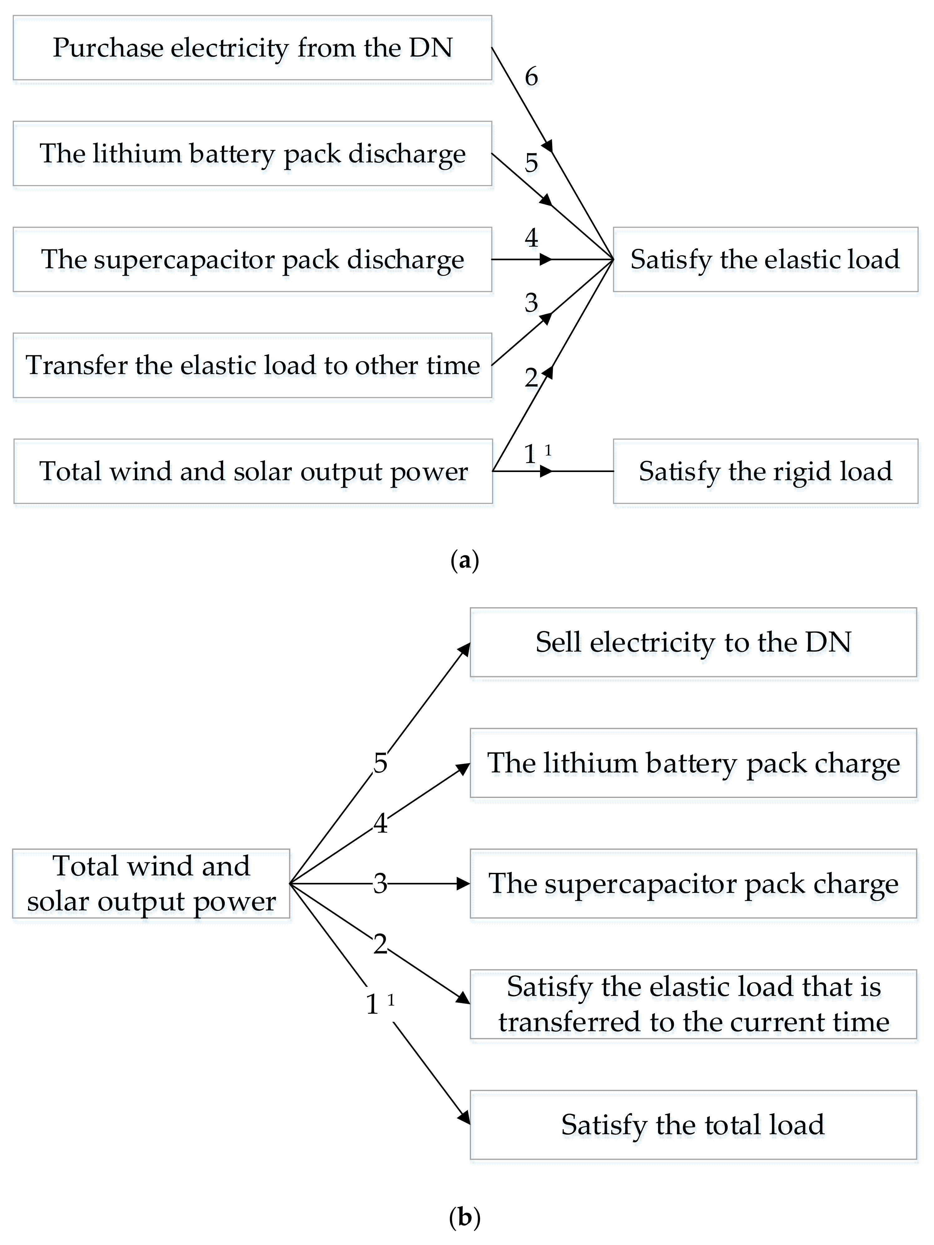
  • Constraints of the supply order of the power and the satisfied order of the load;
There are two situations in which the total wind and solar output power is less than the total load at time t as well as the total wind and solar output power is greater than the total load at time t. There is only one situation at time t. The only one situation at time t refers to: a binary variable U s t is introduced, which represents whether the total wind and solar output power ( P w t t + P p v t ) is greater than the total load ( P l o a d t ) at time t.
U s t = 1 , i f   P w t t + P p v t > P l o a d t 0 , e l s e ,   t = 1 T .
where P w t t + P p v t > P l o a d t represents a situation—the total wind and solar output power is greater than the total load at time t. If this situation happens, U s t takes 1. P w t t + P p v t P l o a d t represents the other situation—the total wind and solar output power is less than the total load at time t. If this situation happens, U s t takes 0. At time t, U s t cannot take 1 and 0 at the same time, that is, there is only one situation at time t. In different situations, the supply order of the power and the satisfied order of the load are different, which can be illustrated from Figure 2.
In Figure 2a, when the total wind and solar output power is less than the total load at time t, the total wind and solar output power is first used to satisfy the rigid load. Then the elastic load is satisfied in accordance with the following order: 1st, the remaining total wind and solar output, 2nd, transferring the elastic load to other moments for electricity consumption, 3rd, the supercapacitor pack discharging, 4th, the lithium battery pack discharging, and 5th, purchasing electricity from the distribution network. In Figure 2b, when the total wind and solar output power is greater than the total load at time t, the total wind and solar output power is absorbed in accordance with the following order. That is, 1st, satisfying the total load, 2nd, satisfying the elastic load transferred to the current time, 3rd, the supercapacitor pack charging, 4th, the lithium battery pack charging, and 5th, selling power to the distribution network.
  • Constraints of power balance;
P w t t + P p v t + P s c d i s t + P b a d i s t + P b u y t = P l o a d t , i f   P g a p t 0 P w t t + P p v t + P s c c h a t + P b a c h a t + P s e l l t = P l o a d t , e l s e w h e r e P b u y t = P b u y , 1 e l a t + P b u y 2 e l a t 0 , P s e l l t < 0 , P g a p t = P l o a d t P w t t + P p v t
P b u y t > 0   & i f   P g a p t > 0   & P s e l l t = 0 , P g a p t P s c d i s t P b a d i s t > 0 P b u y t = 0   & i f   P g a p t 0   & P g a p t P s c d i s t P b a d i s t = 0 P s e l l t = 0 , o r   P g a p t < 0   & P g a p t + P s c c h a t + P b a c h a t = 0 P s e l l t < 0   & i f   P g a p t < 0   & P b u y t = 0 , P g a p t + P s c c h a t + P b a c h a t > 0
P l o a d t = P r i g t + P e l a t , P r i g t = k r i g × P l o a d t
Equation (13) is the power balance constraint. P g a p t is the power gap, a positive value indicates that the total load is greater than the total wind and solar output, and vice versa. P b u y t is the electricity the microgrid purchases from the distribution network, expressed as a positive value. P b u y t equals to the sum of the electricity purchased at the real-time electricity price ( P b u y , 1 e l a t ) and the electricity purchased at the punitive electricity price ( P b u y 2 e l a t ). P s e l l t is the electricity the microgrid sells to the distribution network, expressed as a negative value. In Equation (14), the 1st part, P b u y t > 0   &   P s e l l t = 0 , indicates that when the sum of the total wind and solar output power and the hybrid energy storage devices’ discharge power is less than the load power, consider purchasing electricity from the distribution network; the 2nd part, P b u y t = 0   &   P s e l l t = 0 , indicates that when the sum of the total wind and solar output and the hybrid energy storage devices’ discharge power is sufficient to meet the total load, there is no need for the microgrid to purchase electricity; besides, when the sum of the load and the charge power of hybrid energy storage devices is sufficient to absorb the total wind and solar output, there is no need for the microgrid to sell electricity; and the 3rd part, P s e l l t < 0   &   P b u y t = 0 , indicates that when the sum of the load and the charge power of hybrid energy storage devices is less than the total wind and solar output power, the microgrid sells electricity to the distribution network. P w t t and P p v t are the wind turbine and photovoltaic output power, respectively. P r i g t and P e l a t are the rigid load and elastic load, respectively, and k r i g is the proportion of the rigid load to the total load.
  • Constraints of SOC and charge and discharge power of each energy storage unit;
    S s c , i t = S s c , i t 1 P s c , i c h a   |   d i s t × Δ t E s c S b a , j t = S b a , j t 1 P b a , j c h a   |   d i s t × Δ t E b a  
    S s c m n S s c , i t S s c max , S b a min S b a , j t S b a max
    P s c max P s c , i c h a t 0 < P s c , i d i s t P s c max , P b a max P b a , j c h a t 0 < P b a , j d i s t P b a max
    where S s c , i t and S b a , j t are the state of charge of the ith supercapacitor unit and the jth lithium battery unit at time t, respectively. S s c , i 0 and S b a , j 0 are the initial state of charge of the ith supercapacitor unit and the jth lithium battery unit, respectively. E s c is the rated capacity of the supercapacitor unit. P s c , i c h a   |   d i s t is the charge or discharge power of the ith supercapacitor unit, and P b a , j c h a   |   d i s t is the charge or discharge power of the jth lithium battery unit. S s c max and S s c m n are the upper and lower limits of the state of charge of the supercapacitor unit. S b a max and S b a min are the upper and lower limits of the state of charge of the lithium battery unit. P s c max and P b a max are the upper limits of the discharge power of the supercapacitor unit and the lithium battery unit, respectively. If the charge and discharge power of the energy storage unit is positive, it means discharging, and if it is negative, it means charging.
  • Constraints of continuous and deep charge and discharge of each unit in the lithium battery pack;
    P b a , j c h a t + 1 < 0   & P b a , j d i s t + 1 = 0 , i f   S b a , j t L < S b a , j t L + 1 = = S b a , j t &   S b a min < S b a , j t < S b a max P b a , j d i s t + 1 > 0   & P b a , j c h a t + 1 = 0 , i f   S b a , j t L > S b a , j t L + 1 = = S b a , j t &   S b a min < S b a , j t < S b a max w h e r e t L 1
Among the time before t when the SOC value is not equal to S b a , j t , the time with the shortest distance to t is recorded as (t-L). The meaning of continuous charge and discharge constraints includes two aspects. First, the SOC curve of each unit in the lithium battery pack increases monotonically during the charging process, and there is no midway discharge; Second, the SOC curve of each unit in the lithium battery pack decreases monotonously during the discharging process, and there is no midway charge. In other words, whether a lithium battery unit is charged or discharged at the time (t + 1) depends on its historical SOC changes in addition to the relationship between supply and demand at that time. In equation (19), the continuous charge and discharge constraint is reflected in whether the sign of the charge and discharge power of the lithium battery unit at the time (t + 1) is positive or negative. The meaning of deep charge and discharge constraints includes two aspects. First, the SOC value of each unit in the lithium battery pack starts from S b a min to the end S b a max during the charging process, and each unit in the lithium battery pack cannot be discharged until the SOC value rises to S b a max ; Second, the SOC value of each unit in the lithium battery pack starts from S b a max to the end S b a min during the discharging process, and each unit in the lithium battery pack cannot be charged until the SOC value drops to S b a min . In Equation (19), so long as the SOC of the lithium battery unit at time t is in the open interval S b a min , S b a max , it is necessary to satisfy formula (19), which is a show of the deep charge and discharge constraint.
  • Constraints of demand-side electricity price response;
    P g a p t = P e l a d o w n t + P s c d i s t + P b a d i s t + P b u y , 1 e l a t + P b u y , 2 e l a t , w h e n   P g a p t 0
    ρ e l a t ρ r i g × ξ
Equation (20) expresses that when the total output of the wind and solar is less than the total load, the remaining elastic load after being satisfied by wind and solar output power P g a p t is composed of three parts: 1st, a part transferred to other time ( P e l a d o w n t ), 2nd, hybrid energy storage devices discharge power ( P s c d i s t + P b a d i s t ), and 3rd, a part purchased from the distribution network ( P b u y , 1 e l a t + P b u y , 2 e l a t ). ρ r i g × ξ is the real-time electricity price ceiling, and ξ is the maximum multiple of the real-time electricity price relative to the rigid electricity price.

3.2.3. Solution Algorithm

The three objectives f 1 , f 2 and f 3 are linearly weighted to create a new single goal F .
min F = ω 1 × f 1 f 1 min f 1 max f 1 min + ω 2 × f 2 f 2 min f 2 max f 2 min + ω 3 × f 3 f 3 min f 3 max f 3 min
f 2 max = max t = 1 ~ T P l o a d t min t = 1 ~ T P l o a d t f 3 min = ρ r i g × t = 1 T P l o a d t × Δ t f 1 max = ρ o m , 1 × C max × N b a f 3 max = t = 1 T C u s t f 1 min = f 2 min = 0
C u s t = P l o a d t × ρ r i g × Δ t , i f   P g a p t 0 P w t t + P p v t × ρ r i g × Δ t + Q g a p t × ρ r i g , i f   0 < Q g a p t Q s t e p , 1 l o a d P w t t + P p v t × ρ r i g × Δ t + Q s t e p , 1 l o a d × ρ r i g + Q g a p t Q s t e p , 1 l o a d × ρ r i g + 0.05 , i f   Q s t e p , 1 l o a d < Q g a p t Q s t e p , 2 l o a d P w t t + P p v t × ρ r i g × Δ t + Q s t e p , 1 l o a d × ρ r i g + Q s t e p , 2 l o a d Q s t e p , 1 l o a d × ρ r i g + 0.05 + Q g a p t Q s t e p , 2 l o a d × ρ r i g + 0.3 , i f   Q s t e p , 2 l o a d < Q g a p t Q s t e p , 3 l o a d P w t t + P p v t × ρ r i g × Δ t + Q s t e p , 1 l o a d × ρ r i g + Q s t e p , 2 l o a d Q s t e p , 1 l o a d × ρ r i g + 0.05 + Q s t e p , 3 l o a d Q s t e p , 2 l o a d × ρ r i g + 0.3 + Q g a p t Q s t e p , 3 l o a d × ρ r i g × 2 , i f   Q s t e p , 3 l o a d < Q g a p t Q s t e p , 4 l o a d P w t t + P p v t × ρ r i g × Δ t + Q s t e p , 1 l o a d × ρ r i g + Q s t e p , 2 l o a d Q s t e p , 1 l o a d × ρ r i g + 0.05 + Q s t e p , 3 l o a d Q s t e p , 2 l o a d × ρ r i g + 0.3 + Q s t e p , 4 l o a d Q s t e p , 3 l o a d × ρ r i g × 2 + Q g a p t Q s t e p , 4 l o a d × ρ r i g × 3 , i f   Q s t e p , 4 l o a d < Q g a p t Q s t e p , 5 l o a d P w t t + P p v t × ρ r i g × Δ t + Q s t e p , 1 l o a d × ρ r i g + Q s t e p , 2 l o a d Q s t e p , 1 l o a d × ρ r i g + 0.05 + Q s t e p , 3 l o a d Q s t e p , 2 l o a d × ρ r i g + 0.3 + Q s t e p , 4 l o a d Q s t e p , 3 l o a d × ρ r i g × 2 + Q s t e p , 5 l o a d Q s t e p , 4 l o a d × ρ r i g × 3 + Q g a p t Q s t e p , 5 l o a d × ρ p e l , i f   Q g a p t > Q s t e p , 5 l o a d w h e r e Q g a p t = P g a p t × Δ t
where (1) ω 1 , ω 2 and ω 3 are weights of each sub-goal, i.e., f 1 , f 2 , and f 3 , respectively, whose decision method is to first count the number of papers using each target in the WOS database in the past three years, and then use the judgment matrix method [33] to determine each weight. (2) f 1 min , f 2 min and f 3 min are the minimum values of each sub-goal, i.e., f 1 , f 2 , and f 3 , respectively, and f 1 max , f 2 max and f 3 max are the maximum values of each sub-goal, i.e., f 1 , f 2 , and f 3 , respectively, whose calculation formula is Equation (23). C max represents the maximum daily cycle times of the lithium battery unit. (3) C u s t is the electricity cost of users at time t. Equation (24) indicates that when the total wind and solar output is greater than the total load at time t, the total load is applied to the rigid price. When the total wind and solar output at time t is less than the total load, the part of the total load that is satisfied by the total wind and solar output is applied to the rigid price. While among the total load exceeding the total wind and solar output, i.e., Q g a p t , the parts located in intervals I1, I2, I3, I4, I5 and I6 are applied, respectively, to EP1, EP2, EP3, EP4, EP5 and EP6. I1, the 1st interval, is 0 ,   Q s t e p , 1 l o a d ; I2 is Q s t e p , 1 l o a d ,   Q s t e p , 2 l o a d ; I3 is Q s t e p , 2 l o a d ,   Q s t e p , 3 l o a d ; I4 is Q s t e p , 3 l o a d ,   Q s t e p , 4 l o a d ; I5 is Q s t e p , 4 l o a d ,   Q s t e p , 5 l o a d ; and I6 is Q s t e p , 5 l o a d ,   Q g a p t . EP1, the 1st kind of electricity price, is the rigid electricity price; EP2 is the electricity price after the rigid electricity price increases 0.05 CNY/kWh; EP3 is the electricity price after the rigid electricity price increases 0.3 CNY/kWh; EP4 is the electricity price that is twice the rigid electricity price; EP5 is the electricity price that is 3 multiples of the rigid electricity price; and EP6 is the punitive electricity price. Q s t e p , 1 l o a d , Q s t e p , 2 l o a d , Q s t e p , 3 l o a d , Q s t e p , 4 l o a d and Q s t e p , 5 l o a d are the electricity demarcation points of the step electricity price.
In this paper, the particle swarm algorithm based on natural selection is used to solve the multi-objective optimal dispatching model of the microgrid. A particle swarm algorithm is a kind of heuristic algorithm, which finds the global optimum by following the optimal value currently searched by the particles. The natural selection mechanism is added to the algorithm (that is, the entire particle swarm is sorted by fitness value in each iteration, and the velocity and position of the best half of the particles are used to replace the position and velocity of the worst half) to avoid the algorithm from falling into the local optimum. Using MATLAB software for simulation calculation, the results of multi-objective optimal dispatching of the microgrid are obtained.

4. Results and Discussion

4.1. Data Explanation

The power source, energy storage, and load demand of a microgrid district under the Guizhou Power Grid are configured as follows: 1st, a 2000 kW wind turbine, 2nd, a 1000 kW photovoltaic, 3rd, hybrid energy storage devices composed of a supercapacitor pack and a lithium battery pack, whose parameters are shown in Table 1, and 4th, the load whose daily maximum is 2000 kW. The rigid load accounts for 60% of the total load, i.e., k r i g = 0.6 , and the elastic load refers to air conditioners, washing machines, and so on. The rigid electricity price ρ r i g is 0.5 CNY/kWh. The k in the demand-side electricity price response function is 1.2. The highest multiple of the rigid electricity price ξ is 3, and the penalty electricity price ρ p e l is 5 CNY/kWh. The investment cost per capacity of the lithium battery unit ( ρ i n v ), the operation and maintenance cost coefficient k o m , the interest rate r , the theoretical service life Y e , and the theoretical cycle times n take 2400 CNY/kWh, 12%, 5%, 6 years, and 4500, respectively. The maximum daily cycle times of the lithium battery unit ( C max ) is 15. This paper searched the WOS core collection for articles from 2019 to 2021 in the format of “TS = microgrid and TS = ‘energy storage’ and TS = ‘demand response’”. The statistics show that the number of articles using the aforementioned f 1 , f 2 and f 3 as objective functions is 37, 76, and 45, respectively, and then the target weights ω 1 , ω 2 , ω 3 are calculated to be (0.2342, 0.4810, 0.2848). The electricity demarcation points of the step electricity price, i.e., Q s t e p , 1 l o a d , Q s t e p , 2 l o a d , Q s t e p , 3 l o a d , Q s t e p , 4 l o a d and Q s t e p , 5 l o a d are 50 kWh, 200 kWh, 360 kWh, 400 kWh, and 600 kWh, respectively [34].
Select the wind power, photovoltaic power, and total load power data with a time resolution of 1 min in the summer typical day from 2019 to 2021 of the district. Set the training samples as 1344 groups, and the test samples as 96 groups. The test results of the wind power, photovoltaic power, and total load power based on the BP neural network are shown in Figure 3.
The MAE indicators (see Figure 3) are all small, indicating that the precision of the prediction model is relatively high. In addition, the difference calculation table of the F test is shown in Table 2. It can be seen that for wind power, F = 0.004481, F crit = 3.890867, F < F crit, indicating that the F value is not significant at the level of α = 0.05. That is, there is no significant difference between the actual value and the predicted value at the level of α = 0.05. Therefore, the prediction results have a high degree of credibility. Similarly, the PV power and total load can be analyzed. Finally, it is concluded that the model trained by the BP neural network has a higher prediction accuracy. To sum up, the prediction accuracy of the MAE and F test is relatively high, indicating that the trained model can be used to predict the power of a certain day in the future. Accordingly, this paper uses the model to predict various power with a time resolution of 15 min of the summer typical day in 2022 of the district, and the prediction results are shown in Figure 4.

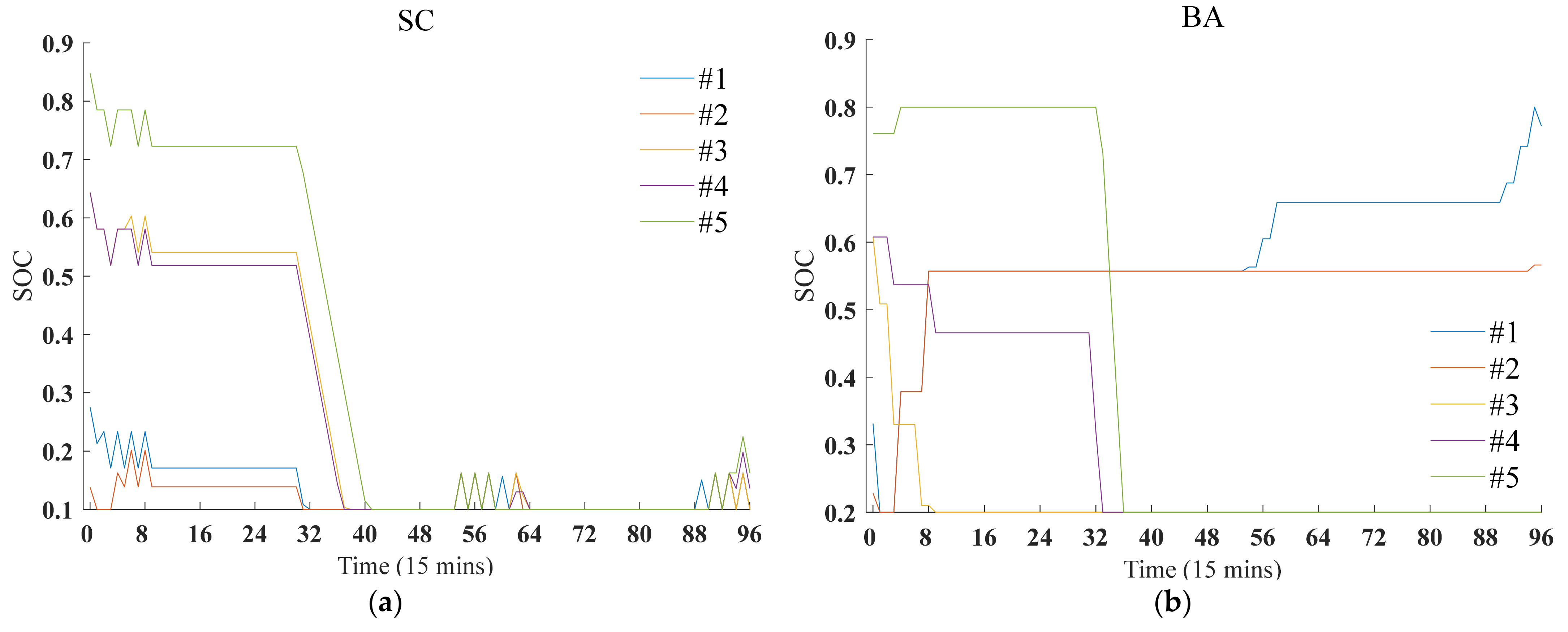
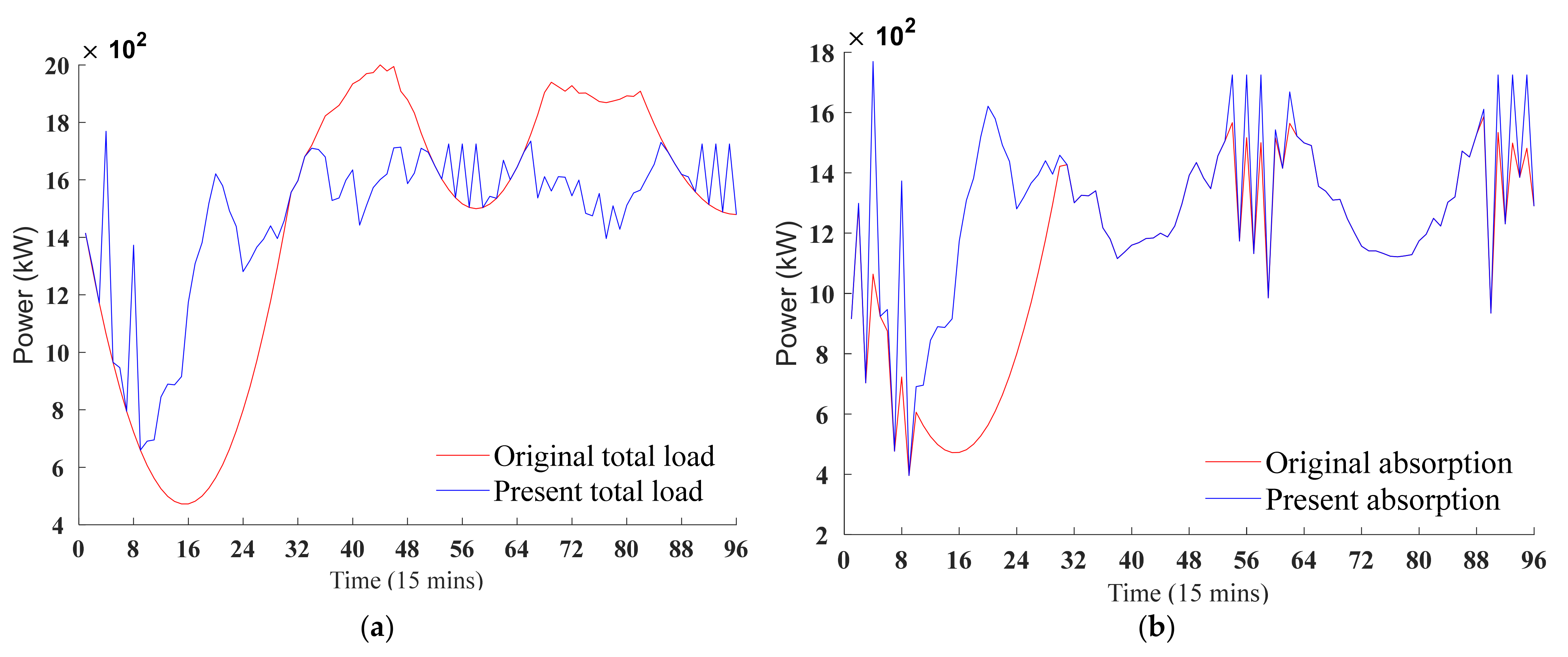
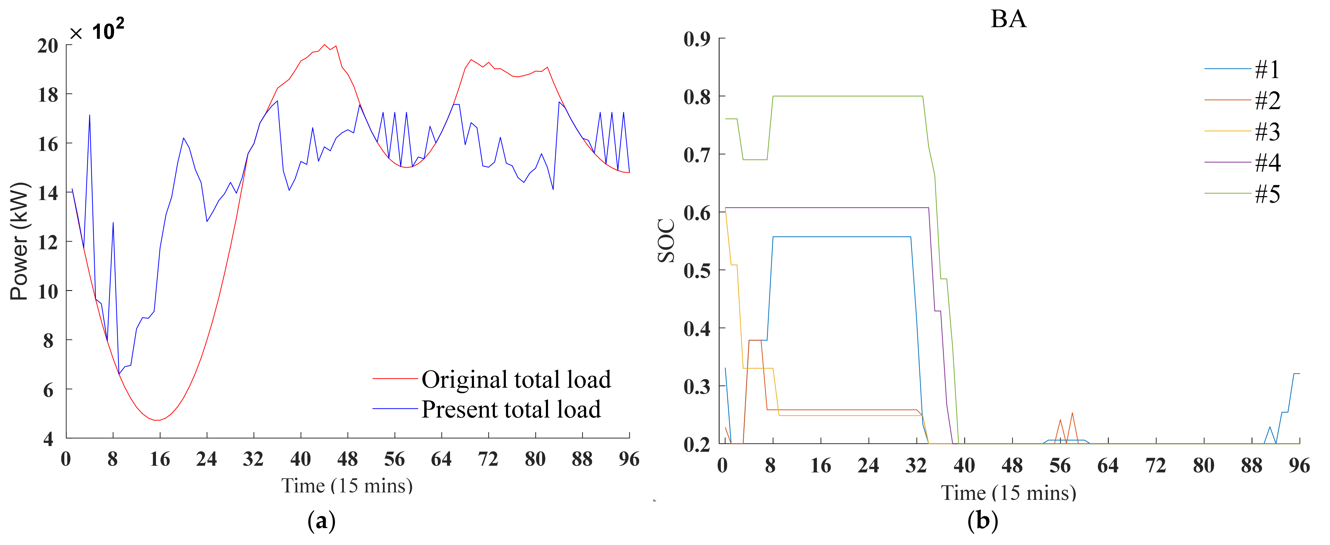
4.2. Optimal Scheduling Results

One of the approaches to absorb the power gap between the total supply and total demand in Figure 4 is the charge and discharge of hybrid energy storage devices. In Figure 5, according to the optimized SOC curve of each energy storage unit, it can be counted that the daily charge and discharge times of each unit in the supercapacitor pack are 15, 11, 10, 10, and 8, respectively; and the daily cycle times of each unit in the lithium battery pack are 2, 1, 1, 1, and 1, respectively. In contrast, the daily cycle times of each lithium battery unit are fewer, which is beneficial to prolong the service life of the lithium battery pack. Besides, because the service life of the lithium battery pack is determined by the unit with the shortest service life in the pack, it is also required that the daily cycle times of each unit in the lithium battery pack are as uniform as possible. Therefore, the result in Figure 5: the ratio of the daily charge and discharge times of each supercapacitor unit to the daily cycle times of each lithium battery unit is reasonable.
(1) In Figure 1 (i.e., the basic framework of a microgrid district under the Guizhou Power Grid), the wind and solar output power is random, volatile, and intermittent, which demands an energy buffer zone. As energy storage devices or to say as an energy storage link, the supercapacitor pack and lithium battery pack come into being. The primary motivation for setting them is purely and simply to weaken to a certain extent and even overcome the aforementioned randomness, volatility, and intermittency on the supply side. When the total wind and solar output power is higher than the load power, the hybrid energy storage devices (i.e., the supercapacitor pack and lithium battery pack) are charged to the utmost according to the surplus wind and solar output power; When the total wind and solar output power is less than the load power, the hybrid energy storage devices are discharged to the utmost according to the remaining load power. Under such a system architecture and engineering background, this paper extracts one day’s data about the wind and solar output power to conduct the experiment. First, the power prediction is made. The wind and solar output power on a certain day in the future is predicted. Then, based on the randomly selected day’s wind and solar output power data, the multi-objective optimization model is solved, and the optimization result in Figure 5 (i.e., SOC curves of hybrid energy storage devices) is obtained. It is within the extracted day that the experiment in this paper is conducted. On a randomly selected day is the deeply important context for making the power prediction and subsequently obtaining the optimal scheduling results. Suppose the extracted day is replaced with another, then the uncertain wind and solar output power on another day will become different rather than repeat itself every day, hence the optimization result in Figure 5 will also change rather than repeat itself every day. (2) On the current randomly selected day, the optimized parameter k in the model of this paper is 1.2. When k takes 1.2, the optimized daily cycle times of the lithium batteries are 2, 1, 1, 1, and 1, respectively, which is beneficial to maximize the service life of the lithium battery pack. If the k is not 1.2, the daily cycle times of the lithium batteries are not 2, 1, 1, 1, or 1, respectively.
Figure 6a shows that after considering the hybrid energy storage devices and demand-side electricity price response, the peak-to-valley difference rate of the daily load curve drops from 76.39% to 62.07%, having a certain effect of peak shaving and valley filling. The drop in peak load (7:30~13:00 and 15:30~21:45) is due to the shift of the elastic load to other times. If the elastic load continues to use electricity at peak hours, the demand-side electricity price response function and the punitive electricity price will be applied, and the electricity cost will be high. If electricity is transferred to other times, the rigid electricity price will be applied, and the electricity cost will be low. In pursuit of minimum electricity cost, the users choose to shift the elastic load to other times. The rise of the valley load (2:15~7:15) is due to the shift of the elastic load to valley hours. With the strong wind and solar output during this period, coupled with the application of the rigid electricity price, the users are driven by economic benefits to shift their elastic load electricity consumption to the period, which not only saves their own electricity cost but also increases the use of renewable energy power generation. In addition, the charge of the hybrid energy storage devices when the wind and solar output is large will also increase the off-peak (refers to the period except 7:30~13:00 and 15:30~21:45) load. In other words, the charge of hybrid energy storage devices is another way to absorb wind and solar power in addition to the elastic load electricity consumption transfer. In Figure 6b, the daily absorption of wind and solar output inside the microgrid increases by 12.72% (see the next paragraph for details). The increase in the consumption of renewable energy in the microgrid is related to the charging of hybrid energy storage and the transfer of flexible load electricity. After optimization, the elastic load shifts from the peak period (7:30~13:00 and 15:30~21:45) of the original electricity consumption to the original electricity consumption’s trough period (2:15~7:15) when the renewable energy output is abundant, thus increasing the consumption of renewable energy output during the valley period, thereby causing the upswing of the consumption curve of renewable energy during the valley period. The charging of hybrid energy storage during periods of sufficient renewable energy output is another reason for the upswing of the renewable energy consumption curve. It can be seen that the transfer of elastic load electricity and the charging and discharging of hybrid energy storage are the common reasons for the change of the load curve (i.e., Figure 6a) and the change of the consumption curve of renewable energy (i.e., Figure 6b). Under the combined effect of the two, the load curve and the renewable energy output curve have a better match in the time dimension.
In the following text, the term “originally” refers to the situation in which the hybrid energy storage devices and demand-side electricity price response are not considered, while the term “now” refers to the situation where they are considered. Three indicators—1st, the daily electricity cost of users, 2nd, the daily electricity purchased from the distribution network, and 3rd, the daily absorption of wind and solar output inside the microgrid—are used to evaluate the improvement effect from originally to now. The daily electricity cost of users was originally 24,019.983 CNY, but now it is 22,572 CNY, a decrease of 6.03%. The daily electricity purchased from the distribution network was originally 7666.970 kWh, but now it is 3972 kWh, a decrease of 48.19%. The daily absorption of wind and solar output inside the microgrid was originally 27,183.092 kWh, but now it is 30,640 kWh, an increase of 12.72%.

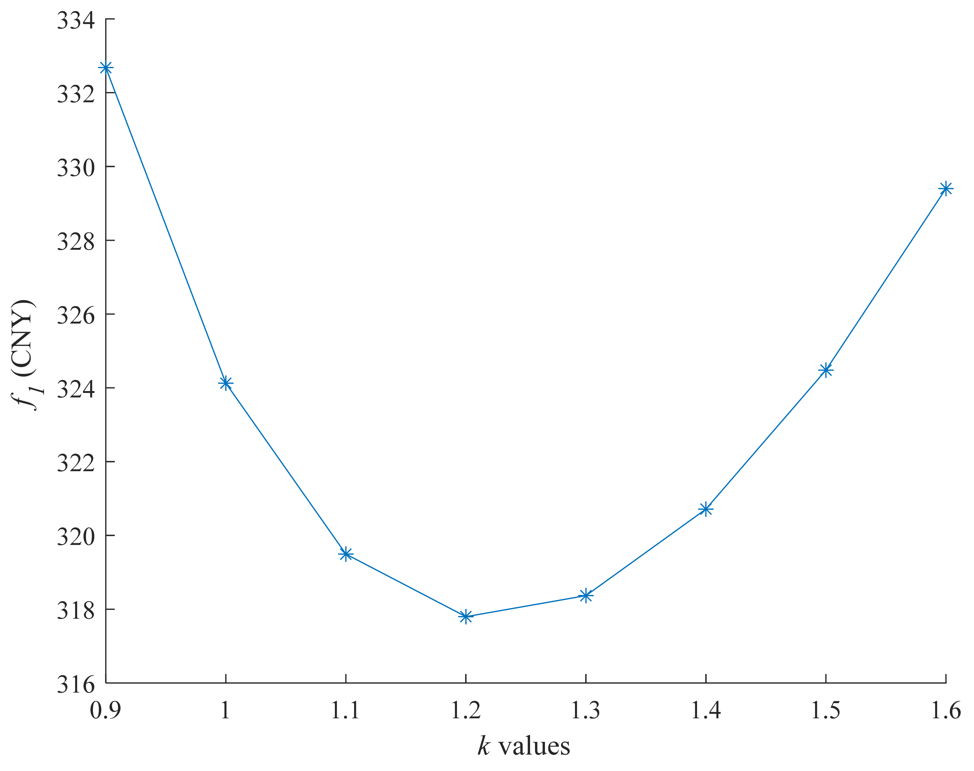
4.3. Sensitivity Analysis

The change of k in the demand-side electricity price response function will cause the change of each sub-objective. It is necessary to find the k that minimizes the daily operation and maintenance cost of the lithium battery pack, i.e., f 1 . When k takes different values, through solving the multi-objective optimization problem, compare the changes of f 1 and take the k that minimizes f 1 . Figure 7 is the comparison of f 1 values under different k values.
When k takes 1.2, f 1 is minimum, which is 317.79 CNY, that is when k in the demand-side electricity price response function takes 1.2, the daily operation and maintenance cost of the lithium battery pack is minimum.
k is the parameter factor in the demand-side electricity price response function. There are two reasons for designing it: (1) The effect of peak-shaving and valley-filling of the load curve is different under different k , and (2) The switching frequency of the energy-type supercapacitor is different from that of the power-type lithium battery under different k . In this paper, k is obtained under the global optimization of supply and demand. The macroeconomic variables can be considered as what the change of k affects, e.g., the influence on the effect of peak-shaving and valley-filling of the load curve as well as the switching frequency of the supercapacitors and the lithium batteries. Under the value of k optimized in this article, 1st, the ratio of the daily charge and discharge times of supercapacitors to the daily cycle times of the lithium batteries is reasonable, 2nd, the absorption of the wind and solar output inside the microgrid increased 12.72%, and 3rd, a certain effect of peak shaving and valley filling of the total load curve is obtained.

4.4. Comparative Analysis

After the optimization model [35] is adopted and solved, the optimization results show that despite a certain effect of peak shaving and valley filling (see Figure 8a), the daily cycle times of each unit in the lithium battery pack are 4, 4, 1, 1, and 2, respectively (see Figure 8b). Correspondingly, the pack’s daily operation and maintenance cost is 2679.3 CNY (while 317.79 CNY in this paper). Compared with the cycle times [1,1,1,1,2] in this paper, the results [4,4,1,1,2] are neither fewer nor uniform. In one day, there exists a saving of the cycle times between [4,4,1,1,2] and [2,1,1,1,1]. Considering that the lithium battery pack is to work for a long term, then the cycle times saving will be considerable one month later or one year later. Therefore, the model in this paper can not only prolong the lithium battery pack’s service life but save its operation and maintenance cost, verifying the superiority of the paper’s model.

5. Conclusions

In this paper, the hybrid energy storage devices and the demand-side electricity price response are utilized to absorb the power gap between supply and demand. At the same time, the reasonable proportion of the daily charge and discharge times of the supercapacitor pack to the daily cycle times of the lithium battery pack has been optimized to maximize the service life of the lithium battery pack. This paper first predicts the renewable energy output and load demand of a microgrid district under the Guizhou Power Grid on a certain day in the future, then performs the multi-objective modeling and solving, and finally obtains the lithium battery pack’s optimal daily charge and discharge strategy as well as the optimal daily elastic load transfer strategy. When the parameter k in the multi-objective model takes 1.2, the daily operation and maintenance cost of the lithium battery pack is minimum. Correspondingly, the ratio of the charge and discharge times of hybrid energy storage devices is reasonable. Also, under the conditions of considering hybrid energy storage devices and the demand-side electricity price response, there occur improvements in three evaluation indicators—the daily electricity cost of users, the daily electricity purchased from the distribution network, and the daily absorption of wind and solar output inside the microgrid. In the future, this article will further study the demand-side electricity price response function to achieve both a better daily load curve peak-shaving and valley-filling effect and the lower electricity cost of users.

Author Contributions

Conceptualization, H.W.; writing—original draft preparation, Y.J.; writing—review and editing, H.W., Y.H. and C.L. All authors have read and agreed to the published version of the manuscript.

Funding

This research was funded by the National Natural Science Foundation of China under Grant No. 52067004.

Institutional Review Board Statement

Not applicable.

Informed Consent Statement

Not applicable.

Data Availability Statement

Not applicable.

Conflicts of Interest

The authors declare no conflict of interest.

Nomenclature

Sets
S e t , 1 ,   S e t , 2 Two different sets of time
Indices
t, s, q, LThe time point
i, jThe ith supercapacitor unit and the jth lithium battery unit, respectively
Superscript
BPBack Propagation
MAEMean absolute error
Variables
ρ o m , 2 The operation and maintenance cost per cycle period of the lithium battery pack
kThe proportional coefficient in the demand-side electricity price response function
ρ e l a t The real-time electricity price at time t
V a The variance of the daily cycle times of lithium battery units
C b a j The daily cycle times of the jth lithium battery unit
P b u y , 1 e l a t The power purchased from the distribution network at the electricity price within the real-time electricity price ceiling at time t
P e l a , 1 t The remaining elastic load at time t
P l o a d a f t t The total load after peak shaving and valley filling at time t
P e l a u p t The elastic load power that is transferred from other time at time t
P e l a d o w n t The elastic load power that is transferred to other moments at time t
P e l a t r a n s , q The amount of the elastic load transfer from time s to time q
P s c c h a t ,   P b a c h a t The charge power of the supercapacitor pack and the lithium battery pack at time t, respectively
P s c , i c h a t ,   P b a , j c h a t The charge power of the ith supercapacitor unit and the jth lithium battery unit at time t, respectively
P s c d i s t ,   P b a d i s t The discharge power of the supercapacitor pack and the lithium battery pack at time t, respectively
P s c , i d i s t ,   P b a , j d i s t The discharge power of the ith supercapacitor unit and the jth lithium battery unit at time t, respectively
P b u y 2 e l a t The power purchased from the distribution network at the punitive electricity price at time t
U s t A binary variable at time t
P b u y t The electricity the microgrid purchases from the distribution network at time t
P s e l l t The electricity the microgrid sells to the distribution network at time t
S s c , i t ,   S b a , j t The state of charge of the ith supercapacitor unit and the jth lithium battery unit at time t, respectively
P s c , i c h a   |   d i s t The charge or discharge power of the ith supercapacitor unit at time t
P b a , j c h a   |   d i s t The charge or discharge power of the jth lithium battery unit at time t
Parameters
N s a The number of test samples
X m The actual value
Y m The predicted value
ρ o m , 1 The fixed operation and maintenance cost per cycle period
N b a The number of units contained in the lithium battery pack
ρ i n v The investment cost per capacity of the lithium battery unit
E b a The rated capacity of the lithium battery unit
k o m The operation and maintenance cost coefficient
r The interest rate
Y e The theoretical service life
n The theoretical cycle times
ρ r i g The rigid electricity price
TA day is divided into T periods
P l o a d t The original total load at time t
N s c The number of units contained in the supercapacitor pack
ρ p e l The punitive electricity price
ΔtThe time interval
P g a p t The power gap at time t
P w t t ,   P p v t The wind turbine and photovoltaic output power at time t, respectively
P r i g t ,   P e l a t The rigid load and elastic load at time t, respectively
k r i g The proportion of the rigid load to the total load
S s c , i 0 ,   S b a , j 0 The initial state of charge of the ith supercapacitor unit and the jth lithium battery unit, respectively
E s c The rated capacity of the supercapacitor unit
S s c max ,   S s c m n The upper and lower limits of the state of charge of the supercapacitor unit
S b a max ,   S b a min The upper and lower limits of the state of charge of the lithium battery unit
P s c max ,   P b a max The upper limits of the discharge power of the supercapacitor unit and the lithium battery unit, respectively
ξ The maximum multiple of the real-time electricity price relative to the rigid electricity price
ω 1 ~ ω 3 Weights of each sub-goal, i.e., f 1 , f 2 , and f 3 , respectively
f 1 min ~ f 3 min The minimum values of each sub-goal, i.e., f 1 , f 2 , and f 3 , respectively
f 1 max ~ f 3 max The maximum values of each sub-goal, i.e., f 1 , f 2 , and f 3 , respectively
C max The maximum daily cycle times of the lithium battery unit
C u s t The electricity cost of users at time t
Q g a p t The total load exceeding the total wind and solar output at time t
Q s t e p , 1 l o a d ~ Q s t e p , 5 l o a d The electricity demarcation points of the step electricity price

References

  1. Jeong, B.C.; Shin, D.H.; Im, J.B.; Park, J.-Y.; Kim, Y.-J. Implementation of Optimal Two-Stage Scheduling of Energy Storage System Based on Big-Data-Driven Forecasting-An Actual Case Study in a Campus Microgrid. Energies 2019, 12, 1124. [Google Scholar] [CrossRef] [Green Version]
  2. Nadeem, F.; Hussain, S.M.S.; Tiwari, P.K.; Goswami, A.K.; Ustun, T.S. Comparative Review of Energy Storage Systems, Their Roles, and Impacts on Future Power Systems. IEEE Access 2019, 7, 4555–4585. [Google Scholar] [CrossRef]
  3. Wu, T.; Ye, F.; Su, Y.; Wang, Y.; Riffat, S. Coordinated Control Strategy of DC Microgrid with Hybrid Energy Storage System to Smooth Power Output Fluctuation. Int. J. Low-Carbon Technol. 2020, 15, 46–54. [Google Scholar] [CrossRef] [Green Version]
  4. Gu, S.; Zhang, J. Two-Stage Stochastic Scheduling Method for Microgrid Based on Price-Based Demand Response. J. North China Electr. Power Univ. 2018, 45, 39–46. (In Chinese) [Google Scholar]
  5. Jin, S.; Mao, Z.; Li, H. Economic Operation Optimization of Smart Micro Grid Considering the Uncertainty. Control Theory Appl. 2018, 35, 1357–1370. (In Chinese) [Google Scholar]
  6. Jin, S.; Mao, Z.; Li, H.; Qi, W. Dynamic Operation Management of a Renewable Microgrid Including Battery Energy Storage. Math. Probl. Eng. 2018, 2018, 5852309. [Google Scholar] [CrossRef] [Green Version]
  7. Liu, Y.; Guo, L.; Wang, C. Economic Dispatch of Microgrid Based on Two Stage Robust Optimization. Proc. CSEE 2018, 38, 4013–4022. (In Chinese) [Google Scholar]
  8. Liu, B.; Zhou, S.; Chen, Y.; Yang, P. Optimal Energy Dispatching Strategy for Microgrid Considering Multi-Scale Demand Response Resources. Electr. Power Constr. 2018, 39, 9–17. (In Chinese) [Google Scholar]
  9. Wang, L.; Wang, X.; Hu, X. Optimal Scheduling of Demand-Side Time-of-Use Pricing Based on the MAS Microgrid. Inf. Control 2020, 49, 429–435. (In Chinese) [Google Scholar]
  10. He, J.; Shi, C.; Ma, M. Bi-Level Optimal Configuration Method of Hybrid Energy Storage System Based on Meta Model Optimization Algorithm. Electr. Power Autom. Equip. 2020, 40, 157–167. (In Chinese) [Google Scholar]
  11. Xu, G.; Shang, C.; Fan, S.; Hu, X.; Cheng, H. A Hierarchical Energy Scheduling Framework of Microgrids with Hybrid Energy Storage Systems. IEEE Access 2018, 6, 2472–2483. [Google Scholar] [CrossRef]
  12. Li, J.; Xiong, R.; Mu, H.; Cornélusse, B.; Vanderbemden, P.; Ernst, D.; Yuan, W. Design and Real-Time Test of a Hybrid Energy Storage System in the Microgrid with the Benefit of Improving the Battery Lifetime. Appl. Energy 2018, 218, 470–478. [Google Scholar] [CrossRef] [Green Version]
  13. Liu, J.; Wei, Q.; Huang, J.; Zhou, W.; Yu, J. Collaboration Strategy and Optimization Model of Wind Farm-Hybrid Energy Storage System for Mitigating Wind Curtailment. Energy Sci. Eng. 2019, 7, 3255–3273. [Google Scholar] [CrossRef]
  14. Wei, M.; Zhou, Q.; Zhou, H.; Cai, S.; Jiang, L.; Lu, L.; Liang, W.; Shen, L.; Li, Q. Economic Dispatch of Microgrid in Southwest China Based on Two-Stage Robust Optimization. Electr. Power 2019, 52, 2–18. (In Chinese) [Google Scholar]
  15. Xu, F.; Liu, J.; Lin, S.; Dai, Q.; Li, C. A Multi-Objective Optimization Model of Hybrid Energy Storage System for Non-Grid-Connected Wind Power: A Case Study in China. Energy 2018, 163, 585–603. [Google Scholar] [CrossRef]
  16. Wang, D.; Qiu, J.; Reedman, L.; Meng, K.; Lai, L.L. Two-Stage Energy Management for Networked Microgrids with High Renewable Penetration. Appl. Energy 2018, 226, 39–48. [Google Scholar] [CrossRef]
  17. Cao, Z.; Han, Y.; Wang, J.; Zhao, Q. Two-Stage Energy Generation Schedule Market Rolling Optimisation of Highly Wind Power Penetrated Microgrids. Int. J. Electr. Power Energy Syst. 2019, 112, 12–27. [Google Scholar] [CrossRef]
  18. Gao, H.-C.; Choi, J.-H.; Yun, S.-Y.; Lee, H.-J.; Ahn, S.-J. Optimal Scheduling and Real-Time Control Schemes of Battery Energy Storage System for Microgrids Considering Contract Demand and Forecast Uncertainty. Energies 2018, 11, 1371. [Google Scholar] [CrossRef] [Green Version]
  19. Kazemi, M.; Zareipour, H. Long-Term Scheduling of Battery Storage Systems in Energy and Regulation Markets Considering Battery’s Lifespan. IEEE Trans. Smart Grid 2018, 9, 6840–6849. [Google Scholar] [CrossRef]
  20. Fan, S.; Qian, A.; Piao, L. Hierarchical Energy Management of Microgrids Including Storage and Demand Response. Energies 2018, 11, 1111. [Google Scholar] [CrossRef] [Green Version]
  21. Li, X.; Ma, R.; Wang, S.; Zhang, Y.; Li, B.; Fang, C. Operation Control Strategy for Energy Storage Station after Considering Battery Life in Commercial Park. High Volt. Eng. 2020, 46, 62–70. (In Chinese) [Google Scholar]
  22. Wei, F.; Sui, Q.; Lin, X.; Li, Z.; Chen, L. Optimized Energy Control Strategy about Daily Operation of Islanded Microgrid with Wind/Photovoltaic/Diesel/Battery under Consideration of Transferable Load Efficiency. Proc. CSEE 2018, 38, 1045–1053. (In Chinese) [Google Scholar]
  23. Lei, M.; Hua, Y.; Zhao, H.; Xu, B. Strategy of Electric Vehicles Participating Peak Load Regulation of Power Grid Considering Battery Life. Mod. Electr. Power 2020, 37, 510–517. (In Chinese) [Google Scholar]
  24. Mohsenian-Rad, H. Optimal Bidding, Scheduling, and Deployment of Battery Systems in California Day-Ahead Energy Market. IEEE Trans. Power Syst. 2016, 31, 442–453. [Google Scholar] [CrossRef] [Green Version]
  25. Global Sustainable Energy Solutions Pty Ltd. Battery Characteristics. In Grid-Connected PV Systems with Battery Storage; China Electric Power Research Institute, Ed.; China Water & Power Press: Beijing, China, 2017; p. 23. [Google Scholar]
  26. He, S.; Gao, H.; Liu, J.; Liu, J. Distributionally Robust Optimal DG Allocation Model Considering Flexible Adjustment of Demand Response. Proc. CSEE 2019, 39, 2253–2264. (In Chinese) [Google Scholar]
  27. Wang, H.; Fang, H.; Yu, X.; Liang, S. How Real Time Pricing Modifies Chinese Households’ Electricity Consumption. J. Clean. Prod. 2018, 178, 776–790. [Google Scholar] [CrossRef]
  28. Wu, N.; Wang, H.; Yin, L.; Yuan, X.; Leng, X. Application Conditions of Bounded Rationality and a Microgrid Energy Management Control Strategy Combining Real-Time Power Price and Demand-Side Response. IEEE Access 2020, 8, 227327–227339. [Google Scholar] [CrossRef]
  29. Krishnamoorthy, M.; Periyanayagam, A.D.V.R. Integrated Energy Management System Employing Pre-Emptive Priority Based Load Scheduling (PEPLS) Approach at Residential Premises. Energy 2019, 186, 115815. [Google Scholar]
  30. Krishnamoorthy, M.; Periyanayagam, A.D.V.R.; Kumar, C.S.; Kumar, B.P.; Srinivasan, S.; Kathiravan, P. Optimal Sizing, Selection, and Techno-Economic Analysis of Battery Storage for PV/BG-based Hybrid Rural Electrification System. IETE J. Res. 2020, 1, 1–16. [Google Scholar] [CrossRef]
  31. Samuelson, P.A.; Nordhaus, W.D. Cost Analysis. In Economics, 18th ed.; Xiao, C., Ed.; Posts & Telecom Press: Beijing, China, 2008; p. 113. [Google Scholar]
  32. Zhang, X.; Yuan, Y.; Cao, Y. Modeling and Scheduling for Battery Energy Storage Station with Consideration of Wearing Costs. Power Syst. Technol. 2017, 41, 1541–1547. (In Chinese) [Google Scholar]
  33. Hu, Y. Practical Multi-Objective Optimization; Shanghai Scientific & Technical Publishers: Shanghai, China, 1987; pp. 60–64. [Google Scholar]
  34. The Step Electricity Price. Available online: https://baike.so.com/doc/5636603-5849230.html (accessed on 1 September 2021).
  35. Wu, T.; Shi, X.; Liao, L.; Zhou, C.; Zhou, H.; Su, Y. A Capacity Configuration Control Strategy to Alleviate Power Fluctuation of Hybrid Energy Storage System Based on Improved Particle Swarm Optimization. Energies 2019, 12, 642. [Google Scholar] [CrossRef] [Green Version]
Figure 1. The basic framework of a microgrid district under the Guizhou Power Grid.
Energies 15 01060 g001
Figure 2. The supply order of the power and the satisfied order of the load. (a) When the total wind and solar output power is less than the total load at time t; (b) When the total wind and solar output power is greater than the total load at time t. 1 The number represents the order, the smaller the number, the more priority the order.
Energies 15 01060 g002
Figure 3. The test results of the wind power, photovoltaic power, and total load power.
Energies 15 01060 g003
Figure 4. The prediction results of the wind and solar output and the total load power.
Energies 15 01060 g004
Figure 5. SOC curves of hybrid energy storage devices. (a) The supercapacitor pack; (b) The lithium battery pack.
Energies 15 01060 g005
Figure 6. The change of the total load curve and the absorption of renewable sources inside the microgrid. (a) The total load curve; (b) The absorption of renewable sources inside the microgrid.
Energies 15 01060 g006
Figure 7. The comparison of f 1 values under different k values.
Energies 15 01060 g007
Figure 8. The optimization results by solving the model in [35]. (a) The change of the total load curve; (b) SOC curve of the lithium battery pack.
Energies 15 01060 g008
Table 1. Parameters of hybrid energy storage devices.
ParametersValues
The   total   number   of   units ,   i . e . ,   N s c   and   N b a 5 and 5
The   rated   power ,   i . e . ,   P s c max   and   P b a max (kW)30 and 250
The   rated   capacity ,   i . e . ,   E s c   and   E b a (kWh)120 and 350
The   upper   limits   of   SOC ,   i . e . ,   S s c max   and   S b a max 0.9 and 0.8
The   lower   limits   of   SOC ,   i . e . ,   S s c min   and   S b a min 0.1 and 0.2
The   initial   SOC   values ,   i . e . ,   S s c , i 0   and   S b a , j 0 (0.27, 0.13, 0.64, 0.64, 0.84) and
(0.33, 0.22, 0.60, 0.60, 0.76)
Table 2. The difference calculation.
Various PowerF 1F crit
Wind power0.0044813.890867
PV power3.16 × 10−73.890867
Total load0.0036163.890867
The judgment method is: when F > F crit, the F value is considered to be significant at the level of α = 0.05.
1 F here is different from F in Section 3.2.3.
Publisher’s Note: MDPI stays neutral with regard to jurisdictional claims in published maps and institutional affiliations.

