Abstract
In this paper, the energy benefits of switchable insulation systems (SIS) are assessed when applied as shades for windows as well as dynamic insulation for exterior walls of residential buildings located in European countries including Belgium and Spain. A series of analyses is performed for detached houses and apartments representing common Belgian residential buildings to determine the energy performance of SIS when deployed to windows and exterior walls and operated using simplified rule-based controls. The analysis results indicate that SIS-integrated windows can achieve significant energy savings for both dwelling types in Belgium, including the elimination of any mechanical cooling and a reduction of up to 44% of heating energy end-use. Moreover, the results show that SIS can offer even more energy efficiency and thermal comfort benefits when deployed to both windows and exterior walls for residential buildings. These energy efficiency benefits are higher, especially for reducing heating needs, for the milder climates of Belgium and Spain. However, it should be noted that the energy performance of SIS could be affected substantially by windows’ orientation and occupants’ behavior.
1. Introduction
Buildings contribute over one-third of the total final energy consumption in Belgium, with the housing stock responsible for 60% of this sectorial demand [1]. Space heating of both single-family and apartment buildings represents over 70% of the total energy consumption of Belgium residential buildings [2]. Several energy efficiency policies and programs have been implemented in Belgium through its regional governments [3] and European Union directives [4] to enhance the energy efficiency of both new and old buildings [5]. In particular, energy efficient design and retrofit measures specific to building envelope systems have been considered, including the use of thermal insulation [6,7,8], the addition of thermal mass [9], and the integration of phase change materials [10,11,12,13,14,15,16]. In Belgium, as in most of Europe, the addition of static thermal insulation has been commonly evaluated to reduce heat transmission through walls and roofs and ultimately lower the energy needed to heat and cool buildings [3]. However, a limited number of analyses have been conducted to assess the energy performance of dynamic insulation, with variable thermal properties, deployed as an alternative to static insulation for the building envelopes. While several technologies have been proposed for dynamic insulation [17], switchable insulation systems (SIS) have been shown to provide substantial energy efficiency benefits for various building envelope elements including walls, roofs, floors, and windows [18]. Specifically, the energy performance of a SIS prototype using rotating insulation layers within a wall cavity has been tested under laboratory conditions [19]. Another experimental study evaluated the performance of switchable, opaque, insulated shading systems when applied to windows [20].
Moreover, the energy benefits of SIS applied to US residential buildings [21] as well as to housing units in Spain [22] have been evaluated. Recently, the energy performance of SIS combined with precooling strategies applied to the roofs of office buildings has been assessed for several US climates [23]. The analysis results have indicated that SIS using simplified two-step control strategies can achieve significant savings in annual heating and cooling energy end-uses reaching up to 65% and 25%, respectively, when considering deploying roof-integrated switchable insulation systems during weekends in addition to weekdays for the various US climates. In addition, the peak electrical demand was reduced by 18% when an SIS was deployed with precooling strategies for an office building located in Denver, CO. Only one study has reported the energy performance of SIS when applied to the walls of residential buildings in Belgium [24]. The study found that SIS when integrated with only the exterior walls of single-family houses and apartment buildings can achieve energy savings up to 3.7% for space heating and up to 98% for space cooling. The heating energy savings can double for SIS-integrated walls with optimally placed thermal mass layers [24]. The energy benefits of SIS for any building can be substantial when applied separately or simultaneously to several elements of the building envelope (i.e., walls, roofs, windows, and floors) as demonstrated by a series of analyses for adaptive insulation systems suitable for US residential buildings [25,26]. In particular, SIS technology has been applied and evaluated separately to exterior walls [21] and roofs/attics [27] for US residential buildings. When SIS were applied simultaneously to both the walls and attics of US detached homes, it was found that they could save up to 22% in annual heating and cooling energy demands [25]. In addition, switchable insulation systems have been applied as shades for standard as well as smart windows to minimize heating and cooling thermal loads for US housing units. In particular, transparent insulating materials are utilized for SIS when deployed as shades and/or blinds for smart windows [26]. Using simplified two-step control rules (i.e., open or closed only), SIS can save up to 59.1% and 64.9% in annual heating and cooling energy, respectively, for houses located in Golden, CO. When optimized controls are considered, SIS can achieve even more energy savings, estimated to be 82% higher compared to the simplified rule set, especially when dwellings are located in hot US climates [28]. Moreover, optimally controlled SIS can reduce electrical peak demand by up to 49.8% compared to the simplified rule set [28].
To date, the impacts of applying dynamic insulation to both walls and windows on the energy performance of buildings have not been evaluated. This study addresses this gap to assess the energy benefits of SIS when deployed to both walls and windows of two housing building types in Belgium. First, the analysis approach is outlined, including the energy models for two common Belgian housing prototypes. Then, the energy performance of SIS is discussed when applied to the walls and windows of both detached houses and apartment buildings located in three cities in Belgium as well as of houses located in Barcelona, Spain. Finally, the impacts of the energy benefits for SIS are investigated when occupant behavior and window orientation are considered.
2. Modeling Approach
In this section, the switchable insulation systems (SIS) applied to windows and walls will be described as well as their operation rule sets. Moreover, the building energy models representing Belgian prototypical detached houses and housing units within apartment buildings are outlined.
2.1. Modeling of SIS Energy Performance
For this study, a simulation environment using resistance and capacitance (RC) thermal networks was used to determine the energy performance of SIS when deployed for building envelope systems. The main advantage of the RC modeling is its flexibility to simulate complex energy systems such as adaptive and switchable building envelope systems as well as the capability to evaluate a wide range of optimized and smart control strategies. A 3R2C (3 resistors–2 capacitors) model was developed for any building envelope systems with SIS and implemented in the MATLAB platform [29], and validated using a state-of-the-art building energy modeling tool, EnergyPlus [30], by Park et al. [17]. Furthermore, a RC-based model was developed for the switchable insulated shade system for windows [26]. The predictions of this model were validated against predictions from EnergyPlus [26].
2.2. SIS-Integrated to Windows and Walls
As noted in the Introduction, the SIS technology considered in this study consists of rotating insulation layers that can be applied to any building envelope elements, including walls [21], windows [26], and roofs/attics [27]. The thermal resistance of the building envelope can be adjusted between high, RH, and low, RL, R-value settings based on the angle, θ, of the rotating insulations layers as illustrated in Figure 1a [19]. Several design configurations and placements are possible to deploy SIS for windows as shading devices and blinds as illustrated in Figure 1 for smart glazing (i.e., Figure 1b) and for standard glazing (Figure 1c) [26]. When applied with smart glazing which can be adjusted to any tint level, SIS are made up of transparent insulation layers [31,32] that are deployed as blinds to allow modulation of the window insulation level as shown in Figure 1b. For standard glazing, SIS include two types of systems consisting of automated opaque shades and transparent insulation layers used as blinds as indicated in Figure 1c. Both systems allow the adjustments of both optical and thermal properties of the windows to be decoupled. Specifically, the switchable blinds made up of transparent insulation layers allow varying the thermal resistance or R-value of the window similar to the SIS effect when deployed within walls and roof/attics [26,27]. The smart glazing and the automated opaque shades for the regular glazing can be controlled to modulate the solar heat gain coefficient (SHGC) of the window.
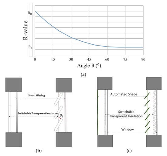
Figure 1.
(a) The variation for SIS as a function of the rotating angle, θ, with configurations for SIS-integrated windows suitable for (b) smart glazing and (c) standard glazing [26].
2.3. SIS Operation Rule Sets
Unlike the case for opaque walls [24], SIS application to windows requires two parameters to be controlled in order to lower the energy used for heating and for cooling (or improved thermal comfort) [26]. These two parameters are the window’s R-value and the window’s SHGC. The simple 2-step rule sets are used to operate SIS-integrated windows and walls as displayed in Figure 2. These rule sets call for the SIS settings of either their thermal properties (i.e., R-value) or their optical characteristics (i.e., SHGC) to take only two values (i.e., either low or high settings) with fully open or closed positions for blinds/shades as well as fully tinted or transparent states for the smart glazing. While the R-value is controlled using the same rule set as the walls, the SHGC value is set based on the HVAC system’s operation mode (i.e., heating, cooling, and dead band).
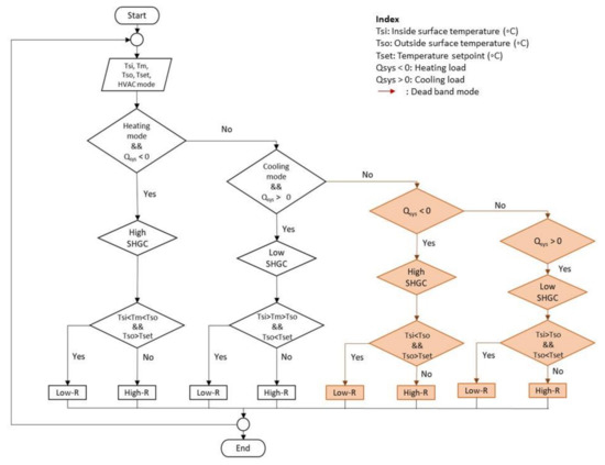
Figure 2.
Rule-based controls used to operate SIS-integrated windows.
2.4. Building Energy Models
In this study, two types of residential buildings, detached houses and apartment units, were considered to represent the vast majority of the Belgian housing stock [2]. Energy models for these two housing types were developed and calibrated [3,24,30]. Figure 3 shows renderings of the energy models for the two building types. Table 1, Table 2 and Table 3 summarize the main features of the two housing energy models [24].
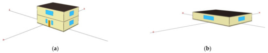
Figure 3.
Rendering for energy models specific to (a) a detached house and (b) an apartment unit.

Table 1.
Characteristics of the modeled apartment and detached house [24].
Table 2.
Internal loads of the prototypical buildings [24].
Table 3.
Thermal properties for building envelope systems [24].
3. Analysis Results
This section summarizes the performance of SIS integrated with the exterior walls and associated windows for both apartment units and detached villas. For exterior walls, the high and low R-values for SIS were 3.9 m2·K/W and 0.49 m2·K/W, respectively. For windows, the high and low R-values were 1.1 m2·K/W and 0.45 m2·K/W, with the high and low SHGCs set to 0.4 and 0.1, respectively. The results are presented for representative days to better evaluate the actions taken by SIS using the rule-based controls outlined in Figure 2 as well as on an annual basis to determine the energy efficiency benefits for SIS. The results specific to SIS-integrated windows and those for combined SIS-integrated windows and walls are discussed separately.
3.1. Performance of SIS-Integrated Windows
In this section, the impacts of SIS-integrated windows are evaluated for two residential building types, including apartment buildings and detached houses.
3.1.1. Apartment Buildings
The performance of SIS-integrated windows associated with the apartment units is detailed for two periods to provide insights on the operation of SIS due to the rule-based controls as well as the weather variations. First, Figure 4 shows the outside and inside surface temperatures for the south window of a prototypical apartment unit located in Brussels during a three-day period ranging from 17 April to 19 April. April is characterized by mild weather conditions in Brussels. Even during this period, however, the outside surface temperature of the window never exceeds that of the internal surface due to the low outdoor temperatures. The window changes its R-value solely due to the HVAC mode rule set outlined in Figure 2. Figure 4 shows that during the three-day period in April (i.e., 17 April–19 April), the HVAC system alternated between heating and dead band modes. When the system operated at the dead band mode, the indoor air temperature was allowed to float and rise above the temperature setpoint as depicted in Figure 5. Therefore, all the windows acted at the same time and remained set at the higher R-value during the entire period. In effect, the R-value setting follows a seasonal pattern as indicated by the rules of Figure 2, used to control the SHGC setting for the SIS-integrated windows.
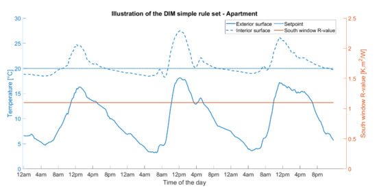
Figure 4.
Performance and settings of SIS deployed on the south window during 17 April to 19 April for the apartment unit. For SIS windows, high R-value = 1.1 m2·K/W; low R-value = 0.45 m2·K/W; high SHGC = 0.4; low SHGC = 0.1.
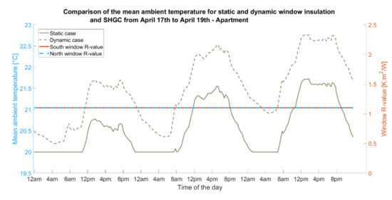
Figure 5.
Indoor air temperature variations for static and dynamic windows during 17 April to 19 April for the apartment unit. For dynamic windows, high R-value = 1.1 m2·K/W; low R-value = 0.45 m2·K/W; high SHGC = 0.4; low SHGC = 0.1. For static windows, R-value = 0.45 m2·K/W; SHGC = 0.4.
During the 17 April to 19 April period, the higher R-value required for the SIS windows allowed the heating needs of the prototypical apartment to be eliminated during this period (i.e., the heating thermal loads were zero for all hours) as shown in Figure 6 when compared to the baseline case of a static window (i.e., R-value = 0.625 m2·K/W). The combined effect of the high R-value setting and of the high SHGC value setting allowed the apartment to benefit from free solar heating and keep its indoor air temperature above the setpoint (i.e., 20 °C) even during nighttime periods, as shown in Figure 5.
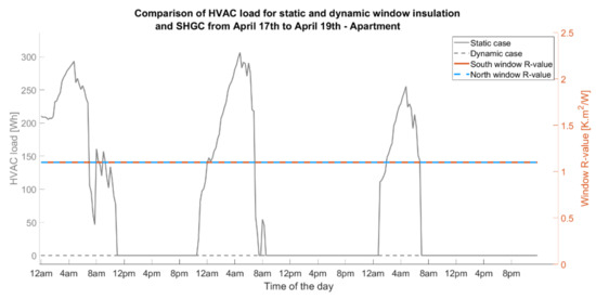
Figure 6.
Comparison of HVAC loads for static and dynamic windows from 17 April to 19 April for the prototypical apartment unit. For dynamic windows, high R-value = 1.1 m2·K/W; low R-value = 0.45 m2·K/W; high SHGC = 0.4; low SHGC = 0.1. For static windows, R-value = 0.45 m2·K/W; SHGC = 0.4.
Figure 7 shows the effect of using SIS-integrated windows on the HVAC energy use for the apartment building when located in Brussels during a three-day period in March (i.e., 4 March to 6 March), characterized by lower outdoor temperatures than April’s three-day period previously evaluated. Due to the higher R-value setting for the dynamic windows, the heating energy required to maintain the indoor thermal comfort (i.e., 20 °C indoor air temperature) decreased. As illustrated in Figure 7, SIS-integrated windows provided a 49.05% reduction in heating energy use compared to the static case during the period from 4 March to 6 March.
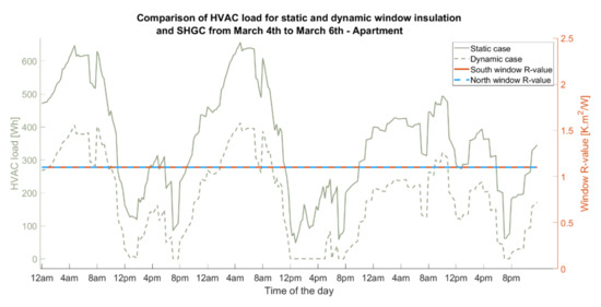
Figure 7.
Comparison of HVAC loads for static and dynamic windows from 4 March to 6 March for the prototypical apartment unit. For dynamic windows, high R-value = 1.1 m2·K/W; low R-value = 0.45 m2·K/W; high SHGC = 0.4; low SHGC = 0.1. For static windows, R-value = 0.45 m2·K/W; SHGC = 0.4.
Figure 8 and Figure 9 present the time variations for both the interior and exterior surface temperatures of the south window during the March three-day period (i.e., 4 March through 6 March). The high R-value and high SHGC setting of the dynamic windows resulted in higher interior surface temperature and lower exterior surface temperature compared to those obtained for the static windows, illustrating the reduced heating thermal loads.
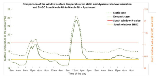
Figure 8.
Interior surface temperature of the south wall for static and dynamic window during 4 March to 6 March for the prototypical apartment unit. For dynamic windows, high R-value = 1.1 m2·K/W; low R-value = 0.45 m2·K/W; high SHGC = 0.4; low SHGC = 0.1. For static windows, R-value = 0.45 m2·K/W; SHGC = 0.4.
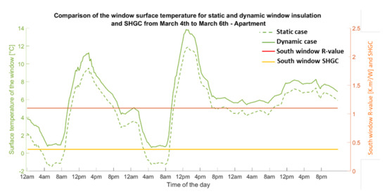
Figure 9.
Exterior surface temperature of the south wall for static and dynamic window during 4 March to 6 March for the prototypical apartment unit. For dynamic windows, high R-value = 1.1 m2·K/W; low R-value = 0.45 m2·K/W; high SHGC = 0.4; low SHGC = 0.1. For static windows, R-value = 0.45 m2·K/W; SHGC = 0.4.
For evaluating the performance of SIS-integrated windows, the baseline case with a low R-value (no insulation) and high SHGC value (no shade) was considered. Using this reference case, the magnitude of energy savings obtained for dynamic windows was generally higher than that achieved by dynamically insulated walls for dwellings located in Brussels [24]. Since dynamic windows can adjust their R-value to a high setting, substantial heating energy savings can occur during the coldest months as indicated in Table 4. Specifically, Table 4 lists the monthly heating energy use for the prototypical apartment with both static and dynamic windows. As shown in Table 4, the dynamic windows can save significant heating energy end-uses for the apartment unit throughout the year ranging from 33.31% in January to 100% in May and October. The annual heating energy saved is estimated to be 44.54% for the dynamic compared to the static (baseline) windows.
Table 4.
Comparison of heating energy consumption for static and dynamic windows for the prototypical apartment unit.
Due to the deployment of SIS-integrated windows, the cooling thermal loads for the apartment unit were eliminated as indicated in Table 5. Due to the seasonal control of the HVAC system, the indoor air temperature dipped very briefly under 20 °C during the cooling season, but otherwise floated between 20 °C and 26 °C. Following the two-step rule set outlined in Figure 2, the SIS windows maintained their low R-value setting during the entire cooling season. Indeed, even when the outside surface temperature of the window was higher than the inside surface temperature, the outside surface temperature never increased past the cooling setpoint (i.e., 26 °C) as illustrated in Figure 10 for a three-day period in April. The SHGC value remained set at the closed position throughout the cooling season. The low settings of both R-value and SHGC for the windows allowed the apartment building to reduce solar heat gains and benefit from free cooling available from lower outdoor temperatures. Indeed, the reduction of the R-value of windows enhanced the heat rejection rate from indoors to outdoors. However, the setting of the windows to have a low SHGC decreased the access to outdoor views for the occupants as the windows were set at their tinted state for the smart glazing case (i.e., Figure 1b) or the automated shades were fully deployed for the standard glazing configuration (i.e., Figure 1c). Consequently, no exterior light could enter the dwelling and the occupants could not see the exterior views. An automated schedule could be set to restrict the periods when SIS-integrated windows are allowed to be fully closed as will be discussed in Section 4.
Table 5.
Comparison of cooling energy consumption for static and dynamic windows for the prototypical apartment unit.
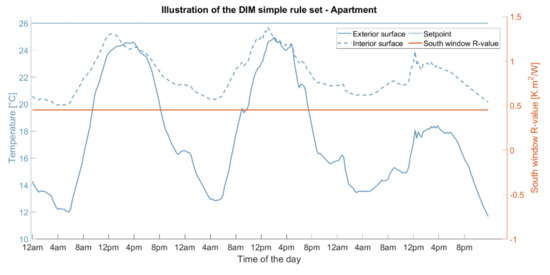
Figure 10.
R-value and surface temperature variations using the simple rule set for SIS south window during the cooling season. For SIS windows, high R-value = 1.1 m2·K/W; low R-value = 0.45 m2·K/W; high SHGC = 0.4; low SHGC = 0.1.
3.1.2. Detached House
The application of SIS-integrated windows to the prototypical detached house decreased the annual space heating energy consumption by 30.95% when compared to the baseline static windows case as summarized in Table 6. While the relative savings were smaller than in the case of the prototypical apartment unit, the absolute savings were much larger. These annual space heating energy savings amounted to 3613 kWh, which is more than 1.5 times the space heating energy consumption of the prototypical apartment unit. Due to the increased window insulation, the application of SIS-integrated windows was most beneficial during the colder months for the detached house. Indeed, more than 45% of the annual savings were achieved during the months of January, February, and December. The heating energy savings increased during the shoulder months compared to the colder months as longer daytime periods increase the dwelling’s solar heat gains.
Table 6.
Comparison of heating energy consumption for static and dynamic windows for the prototypical detached house.
As presented in Table 7, SIS-integrated windows eliminated the prototypical detached house’s cooling needs for the Belgian climates as the result of the combined effect of the lower R-value and low SHGC value settings. These savings are attributed mainly to the lower SHGC value setting allowed by the SIS-integrated windows, which reduced the solar gains of the dwelling compared to the static window case.
Table 7.
Comparison of cooling energy consumption for static and SIS-integrated windows for the prototypical detached house.
3.2. SIS Integrated in Both Walls and Windows
In the previous section, only some of the effects of SIS-integrated windows were evaluated by analyzing the annual space heating and cooling energy for two prototypical Belgian residential buildings. The impacts of SIS when integrated in both exterior walls and windows are investigated in this section. Specifically, Table 8 presents the annual space heating and cooling energy end-uses when both prototypical dwellings were fitted with SIS-integrated walls and SIS-integrated windows. The configuration of Figure 1b was considered for SIS-integrated windows in this analysis. Thus, the window insulation layer was assumed to be transparent and the glazing to be smart, so the controls of both the SHGC and U-value (or R-value) for the fenestration system can be decoupled. The yearly space heating energy consumption of the detached house was lower for the SIS combined integration to walls and windows than the sum of savings obtained for the SIS separately integrated in walls only and in windows only. Specifically, the annual heating energy savings were estimated to be 31.69%, which was slightly less than the sum of the two separate SIS savings (32.12%) due to the interactive effects between the SIS-integrated walls and SIS-integrated windows. These interactive effects are attributed to the fact that heat transfer is reduced when the temperature gradient between the inside and the exterior of the dwelling decreases.
Table 8.
Comparison of heating and cooling energy consumption for static and SIS windows and walls for the prototypical detached house and apartment.
When compared with the performance specific to the SIS-integrated windows only case, the cooling energy savings obtained by the SIS combined integration to the walls and windows and the cooling energy savings of the prototypical apartment unit and detached house were slightly decreased as shown in Table 8. This result can be attributed to the seasonal change in HVAC controls, which were not optimally operated. The building envelope elements stored more heat due to the combined actions of both the walls and windows and thus required lower cooling energy demands.
4. Sensitivity Analysis
In this section, the impacts of SIS integrated walls and windows are determined for various climates as well as operation conditions including orientations and restrictive operation settings for the windows to account for occupant behaviors.
4.1. Impact of Climate
4.1.1. Belgian Climate Zones
Three locations were considered in Belgium to represent different climate zones, including Brussels in the middle of the country, Oostende on the coastline, and St Hubert in the Ardennes. Heating and cooling degree-days of the three locations are presented in Table 9 as well as the average, minimum, and maximum yearly temperature. Located on the coastline, Oostende’s climate is affected strongly by the sea, resulting in smaller variations in temperature than in the climates of Brussels and St Hubert, which are further inland. Indeed, Brussels is characterized by large temperature fluctuations both during the winter and during the summer seasons. Meanwhile, St Hubert’s climate is dryer and has colder temperatures as it is farther from the sea than the other two locations.
Table 9.
Summary of weather conditions for three cities representative of different climates in Belgium.
Table 10 presents the space heating and cooling energy savings when both SIS walls and SIS windows were deployed for the two prototypical dwellings located in the three locations representative of the various climate zones in Belgium. As with the results obtained when SIS-integrated windows were considered, the cooling energy demands and thus the needs of the air conditioning systems in both dwellings were eliminated for all three locations. For all three locations, however, applying SIS-integrated walls in addition to the SIS-integrated windows yielded only slight additional heating energy savings of less than 1% for the detached houses and between 1.3% and 2% for the apartment units.
Table 10.
Annual heating and cooling energy consumption for static and SIS walls and windows applied to two prototypical dwellings for three climates in Belgium.
4.1.2. Barcelona, Spain
The energy performance of combined SIS integration to walls and windows was evaluated for the prototypical detached house located in Barcelona, Spain, as it experiences a warmer climate that any of sites considered for Belgium. Indeed, SIS-integrated walls have been reported to be more effective in milder climates for residential and commercial buildings [1,2].
Table 11 lists the annual space heating and cooling energy consumption when the detached house is located in Barcelona for various design configurations, including static walls and windows, separate SIS-integrated walls and SIS-integrated windows cases, and finally combined SIS integration to both walls and windows. Due to the warmer climate of Barcelona, the heating energy savings were larger than those estimated for Brussels. Indeed, a reduction of 4.70% in heating energy end-use was obtained in Barcelona when applying SIS-integrated walls to the detached house compared to the 1.17% savings achieved in Brussels. Moreover, the application of SIS-integrated windows in Barcelona reduced the dwelling’s heating needs by 60.35% due mostly to the better window insulation level associated with the high R-value setting. The combined SIS integration to walls and windows reduced the heating energy consumption of the detached house further to 62.88% relative to the baseline static case. These relative heating energy savings were double those obtained for Brussels (31.69%), mostly due to the milder winters in Barcelona which allow for more free heating opportunities (i.e., contribution of SIS-integration walls) and less heat losses through the building envelope (i.e., contribution of SIS-integrated windows). When deployed for walls and windows, SIS could almost entirely eliminate the annual cooling thermal load for the detached house located in Barcelona as indicated by the results of Table 11.
Table 11.
Annual heating and cooling energy consumption for static and SIS walls and windows applied to a detached house in Barcelona, Spain.
Figure 11, Figure 12 and Figure 13 illustrate the specific actions due to the rule-based controls when deploying SIS-integrated walls only (Figure 11), SIS-integrated windows only (Figure 12), as well as both SIS-integrated walls and windows (Figure 13) for a period of three summer days (22 July to 24 July). For all cases, the north window exterior and interior surface temperatures are shown for easy comparative analysis of the impact of SIS-integrated windows. Moreover, the north wall and window’s actions are illustrated in Figure 11, Figure 12 and Figure 13 since they were determined to be the most effective during the cooling season. As indicated in Figure 11, the north wall periodically selected its low R-value during nighttime periods to allow for free cooling and its high R-value during the daytime hours to reduce the house’s cooling thermal load. Figure 12 shows that the SIS-integrated north window also selected its low R-value during the night and switched to its high R-value setting when the window’s outside surface temperature became higher than the internal surface temperature or the temperature setpoint as called for by the rules of Figure 2.
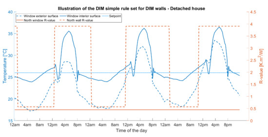
Figure 11.
Performance of SIS walls only case during the period between 22 July to 24 July for the prototypical detached house located in Barcelona, Spain. For SIS walls and dynamic windows, high R-value = 3.9 m2·K/W; low R-value = 0.49 m2·K/W. For SIS windows, high R-value = 1.1 m2·K/W; low R-value = 0.45 m2·K/W; high SHGC = 0.4; low SHGC = 0.1.
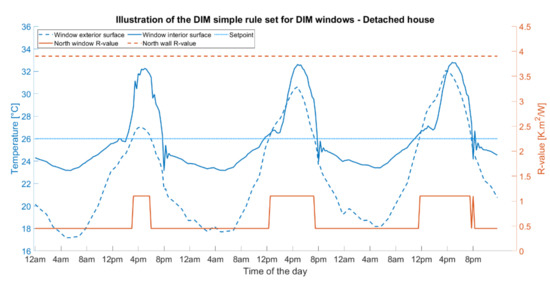
Figure 12.
Performance of SIS windows only case during the period between 22 July to 24 July for the prototypical detached house located in Barcelona, Spain. For SIS windows, high R-value = 1.1 m2·K/W; low R-value = 0.45 m2·K/W; high SHGC = 0.4; low SHGC = 0.1. For static walls, R-value = 3.9 m2·K/W.
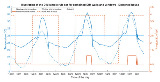
Figure 13.
Performance of combined SIS walls and windows during the period between 22 July to 24 July for the prototypical detached house located in Barcelona, Spain. For SIS walls and dynamic windows, high R-value = 3.9 m2·K/W; low R-value = 0.49 m2·K/W. For SIS windows, high R-value = 1.1 m2·K/W; low R-value = 0.45 m2·K/W; high SHGC = 0.4; low SHGC = 0.1.
Figure 13 presents the effects of deploying both SIS-integrated walls and SIS-integrated windows during a three-day summer period between 22 July and 24 July. When compared to the separate SIS cases, both the north wall and north window maintained their high R-value for a shorter period, mostly by switching to the high R-value setting later during the day. The combined effect of nighttime free cooling lowered the temperatures of the walls and the indoor air more significantly than it does for the SIS separate cases. Thus, the window and wall interior surface temperatures remained lower for longer periods.
4.2. Impact of Operation of Windows
Effect of Orientation for SIS-Integrated Windows
If the SIS-integrated windows are set to their low SHGC value through having a fully tinted state for the smart glazing (Figure 1b) or closing the automated opaque shades as outlined for the standard glazing configuration (Figure 1c), the dwelling occupants’ access to outdoor views can be greatly reduced and even obstructed. In this section, the impact of forcing the SIS-integrated windows to remain open during the daytime periods to allow occupants to have access to outdoor views as well as to natural light is investigated. Specifically, the case of the combined SIS integration to walls and windows is considered when three out of the four windows of the detached house were forced by occupants to be set open from 7:00 a.m. to 7:00 p.m. to readily access outdoor views from most rooms within the dwelling. During the heating season, only the north window was allowed to activate following the SIS-integrated window two-step rule sets during the day, while during the summer season, only the south window followed the two-step rule set during the day.
Table 12 shows the heating and energy savings obtained for the combined SIS case, the restricted SIS windows case (i.e., only one SIS-integrated window is operated), and the unrestricted SIS case (i.e., all SIS-integrated windows are operated) compared to the static baseline case. The space heating energy savings amounted to 30.95% for unrestricted SIS walls and windows but decreased to 20.65% for the restricted case. The SIS walls had a small contribution to the heating energy savings for both the restricted and unrestricted operation of the windows. For the cooling energy demand, the contribution of the SIS walls was more significant due to the small magnitude of the thermal cooling load for the house located in Brussels. As shown in Table 12, when three out of four SIS windows were forced open during the daytime periods throughout the year, the prototypical house’s cooling energy needs amounted to 25.31 kWh; when SIS walls were applied to this case, the estimated cooling needs decreased to 9.94 kWh.
Table 12.
Comparison of annual space heating and cooling energy consumption when a single window of the prototypical detached house model is forced open during the morning.
When SIS-integrated shades were forced open during noon periods, the south-oriented windows achieved the greatest savings (12.50%) as shown in Table 13. Comparatively, the east and west-oriented windows achieved annual energy savings of 8.99% and 9.00%, respectively, while the north windows provided 8.82%. From the results of Table 13, it can be concluded that rooms with a high occupation rate in the dwelling around noon should have windows facing south to maximize energy savings while allowing occupants to have a flexible accessibility to the outdoor views.
Table 13.
Comparison of annual space heating and cooling energy consumption when a single window of the prototypical detached house model is forced open around noon.
Table 14 displays the annual energy consumption of the prototypical house when a single SIS-integrated window was forced open during the afternoon period (i.e., 2:00 p.m. to 5:00 p.m.) daily throughout the year. Keeping the west or south windows open during the afternoon period gave greater annual energy savings—of 9.93% and 9.86%, respectively—than those achieved when the east or north SIS-integrated windows were restricted. These higher savings are attributed to the increased solar exposure of the south and west windows during the afternoon periods. This result indicates that rooms generally occupied during the afternoon periods should have SIS-integrated windows facing west and/or south.
Table 14.
Comparison of annual space heating and cooling energy consumption when a single window of the prototypical detached house model is forced open during the afternoon.
Table 15 presents the annual HVAC energy consumption when forcing one SIS-integrated window to remain open during the evening period (i.e., 5:00 p.m. to 8:00 p.m.). Due to Brussels’ relatively high latitude, the sun sets quite early (4:30 p.m. at the earliest) during the winter season. Thus, keeping the windows open during the winter months would offer no benefits from solar heat gains. However, in the shoulder months, the sun sets as late as 10:00 p.m. Since the sun sets in the west, the west window is the last window of the house to benefit from potential solar gains. Therefore, west-oriented SIS-integrated windows had the highest annual energy savings among all orientations (7.69%). It should be noted that the energy performance for other oriented windows was similar with equal annual savings due to SIS deployment (7.30%). Thus, rooms which are occupied during the evenings should have west-facing windows.
Table 15.
Comparison of annual space heating and cooling energy consumption when a single window of the prototypical detached house model is forced open during the evening.
5. Conclusions
The results of the study summarized in this paper confirm that switchable insulation systems (SIS) integrated as dynamic shades for windows as well as a dynamic insulation layer for exterior walls can significantly reduce heating and cooling energy demands for residential buildings in Belgium and Spain. The impact of SIS integrated with windows was found to be more significant than that of SIS integrated with walls for both detached houses and apartment buildings due to the cold climate throughout Belgium. Indeed, SIS when deployed as dynamic shades for windows eliminated the entire cooling thermal load and thus the need for any air conditioning system as well as achieved an over 45% reduction in heating energy needs. The SIS integrated walls slightly increased the heating energy savings by an additional 1%–3% depending on the climate zone in Belgium. For detached houses located in milder European climates such as that of Spain, the energy efficiency benefits of SIS were even higher, with over 62% reduction in heating energy end-use in addition to the elimination of cooling energy demand. Thus, the deployment of SIS for residential buildings in several European climates can avoid the installation of air conditioning equipment, representing significant reductions in both construction capital costs and carbon emissions.
The impacts of occupant behaviors on the performance of SIS-integrated windows were evaluated as part of the series of analyses carried out in the study. The results indicate that the desire of occupants to access outdoor views can reduce the energy benefits of SIS-integrated windows. However, the magnitude of this reduction depends significantly on the specific restriction period and the orientation of the SIS-integrated windows. Based on the results of the analyses presented in this study, optimized room placement within dwellings can be considered to maximize both the flexibility for occupant-based window operations and the energy efficiency of space heating and cooling systems. The recommendations that follow are principally specific to dwellings located in Belgium but could be applied to locations with a similar cold climate. Using occupancy patterns for Belgian households, bedrooms are occupied mostly at night and in the early morning, while the living rooms and office spaces are mostly occupied throughout the daytime periods. Kitchen spaces can be used during various periods including morning, noon, and evening. Using SIS technology, north-oriented windows should be kept closed most of the year. Thus, rooms that have a limited occupancy during the daytime should have northern-facing windows or even have no windows. Such rooms include garages, restrooms, bathrooms, and laundry rooms. Windows for bedrooms can be facing east, west, or south. The living room, the kitchen, and the office should have south-oriented windows.
Future work can include optimized controls for SIS when integrated to windows and walls as well as field testing on the energy performance of buildings equipped with the technology. In addition, the energy benefits of SIS applied to other building types including office buildings could be assessed as a part of future studies.
Author Contributions
Conceptualization, M.K.; methodology, M.K.; software, M.D. and R.C.; validation, R.C.; formal analysis, R.C.; investigation, R.C.; resources, M.K.; data curation, R.C.; writing—original draft preparation, R.C.; writing—review and editing, M.K.; visualization, R.C.; supervision, M.K.; project administration, M.K.; funding acquisition, R.C. All authors have read and agreed to the published version of the manuscript.
Funding
This research received no external funding.
Conflicts of Interest
The authors declare no conflict of interest.
Nomenclature
| ACH | Air change per hour |
| ASHRAE | American Society of Heating, Refrigerating and Air-Conditioning Engineers |
| CDD | Cooling degree days with 18 °C base temperature (°C-day/year) |
| COP | Coefficient of performance of the air conditioning system |
| DHW | Domestic hot water |
| HDD | Heating degree days with 18 °C base temperature (°C-day/year) |
| HVAC | Heating ventilation and air conditioning |
| HVAC load | Heat transferred to or from the HVAC system (kWh) |
| KWh | Kilowatt-hour |
| R-value | Thermal resistance (m2·K/W) |
| RH | High setting for SIS thermal resistance (m2·K/W) |
| RL | Low setting for SIS thermal resistance (m2·K/W) |
| RC | Resistor–capacitor |
| SHGC | Solar heat gain coefficient |
| SIS | Switchable insulation system |
| U-value | Thermal transmittance (W/m2·K) |
| WWR | Windows-to-wall ratio |
References
- Economie. Energy Key Data 2016—Belgium; Jean-Marc Delporte: Brussels, Belgium, 2016; Volume 5, p. 3. [Google Scholar]
- Lodewijckx, E.; Deboosere, P. Ménages et Familles: Evolutions Rapides et Grande Stabilité à la Fois. Available online: https://ggps.be/doc/GGP_Belgium_Paper_Series_6-FR.pdf (accessed on 31 March 2020).
- Cyx, W.; Renders, N.; van Holm, M.; Verbeke, S. IEE TABULA—Typology Approach for Building Stock Energy Assessment. Mol Belgium; Intelligent Energy Europe: Loughborough, UK, 2011. Available online: https://episcope.eu/fileadmin/tabula/public/docs/scientific/BE_TABULA_ScientificReport_VITO.pdf (accessed on 31 March 2020).
- PEN. Performance Énergétique des Bâtiments (PEN 2017)—Energie Plus le Site. Available online: https://energieplus-lesite.be/reglementations/le-batiment3/performance-energetique-des-batiments-pen-2017/ (accessed on 31 March 2020).
- Ruellan, G. La Rénovation du Bâti Résidentiel en Belgique; ULg: Liège, Belgium, 2016. [Google Scholar]
- Kossecka, E.; Kosny, J. Influence of insulation configuration on heating and cooling loads in a continuously used building. Energy Build. 2002, 34, 321–331. [Google Scholar] [CrossRef]
- Aissani, A. Optimisation Fiabiliste des Performances Énergétiques des Bâtiments. Ph.D. Thesis, Université Blaise Pascal-Clermont-Ferrand II, Landais, France, 2016. [Google Scholar]
- Sambou, V. Optimisation Thermique et Étude Thermodynamique d’une Paroi de Bâtiment. Ph.D. Thesis, Université de Toulouse, Toulouse, France, 2008. [Google Scholar]
- Nicolas, J.; Andre, P.; Rivez, J.; Debbaut, V. L’inertie dans la maison individuelle: Un gain de consommation énergétique? Simulation et étude de cas. Rev. Générale Therm. 1991, 30, 240–249. [Google Scholar]
- de Gracia, A.; Navarro, L.; Castell, A.; Ruiz-Pardo, Á.; Alvárez, S.; Cabeza, L.F. Experimental study of a ventilated facade with PCM during winter period. Energy Build. 2013, 58, 324–332. [Google Scholar] [CrossRef]
- de Gracia, A.; Navarro, L.; Castell, A.; Cabeza, L.F. Energy performance of a ventilated double skin facade with PCM under different climates. Energy Build. 2015, 91, 37–42. [Google Scholar] [CrossRef] [Green Version]
- Soares, N.; Costa, J.J.; Gaspar, A.R.; Santos, P. Review of passive PCM latent heat thermal energy storage systems towards buildings’ energy efficiency. Energy Build. 2013, 59, 82–103. [Google Scholar] [CrossRef]
- Soares, N.; Gaspar, A.R.; Santos, P.; Costa, J.J. Multi-dimensional optimization of the incorporation of PCM-drywalls in lightweight steel-framed residential buildings in different climates. Energy Build. 2014, 70, 411–421. [Google Scholar] [CrossRef]
- Diaconu, B.M.; Cruceru, M. Novel concept of composite phase change material wall system for year-round thermal energy savings. Energy Build. 2010, 42, 1759–1772. [Google Scholar] [CrossRef]
- Kuznik, F.; Virgone, J.; Johannes, K. In-situ study of thermal comfort enhancement in a renovated building equipped with phase change material wallboard. Renew. Energy 2011, 6, 1458–1462. [Google Scholar] [CrossRef] [Green Version]
- Mandilaras, I.; Stamatiadou, M.; Katsourinis, D.; Zannis, G.; Founti, M. Experimental thermal characterization of a Mediterranean residential building with PCM gypsum board walls. Build. Environ. 2013, 61, 93–103. [Google Scholar] [CrossRef]
- Park, B.; Srubar, W.V.; Krarti, M. Energy performance analysis of variable thermal resistance envelopes in residential buildings. Energy Build. 2015, 103, 317–325. [Google Scholar] [CrossRef]
- Dehwah, A.H.A.; Krarti, M. Impact of switchable roof insulation on energy performance of US residential buildings. Build. Environ. 2020, 177, 106882. [Google Scholar] [CrossRef]
- Dabbagh, M.; Krarti, M. Evaluation of the performance for a dynamic insulation system suitable for switchable building envelope. Energy Build. 2020, 222, 110025. [Google Scholar] [CrossRef]
- Dabbagh, M.; Krarti, M. Experimental evaluation of the performance for switchable insulated shading systems. Energy Build. 2022, 256, 111753. [Google Scholar] [CrossRef]
- Menyhart, K.; Krarti, M. Potential energy savings from deployment of Dynamic Insulation Materials for US residential buildings. Build. Environ. 2017, 114, 203–218. [Google Scholar] [CrossRef]
- Garriga, S.M.; Dabbagh, M.; Krarti, M. Evaluation of Dynamic Insulation Systems for Residential Buildings in Barcelona, Spain. ASME J. Eng. Sustain. Build. Cities 2020, 1, 011002. [Google Scholar] [CrossRef]
- Dehwah, A.H.A.; Krarti, M. Performance of precooling strategies using switchable insulation systems for commercial buildings. Appl. Energy 2021, 303, 117631. [Google Scholar] [CrossRef]
- Carlier, R.; Dabbagh, M.; Krarti, M. Impact of Wall Constructions on Energy Performance of Switchable Insulation Systems. Energies 2020, 13, 6068. [Google Scholar] [CrossRef]
- Dehwah, A.H.A.; Krarti, M. Energy Performance of Integrated Adaptive Envelope Systems for Residential Buildings. Energy 2021, 233, 121165. [Google Scholar] [CrossRef]
- Dabagh, M.; Krarti, M. Energy Performance of Switchable Window Insulated Shades for US Residential Buildings. J. Build. Eng. 2021, 43, 102584. [Google Scholar] [CrossRef]
- Dehwah, A.H.A.; Krarti, M. Cost-benefit analysis of retrofitting attic-integrated switchable insulation systems of existing US residential buildings. Energy 2021, 221, 119840. [Google Scholar] [CrossRef]
- Dabagh, M.; Krarti, M. Optimal Control Strategies for Switchable Transparent Insulation Systems Applied to Smart Windows for US Residential Buildings. Energies 2021, 14, 2917. [Google Scholar] [CrossRef]
- MATLAB, 9.7.0.1190202 (R2020a); The MathWorks Inc.: Natick, MA, USA, 2020.
- EnergyPlus, EnergyPlusTM, version 9.5.0; Documentation: Engineering Reference; US Department of Energy: Washington, DC, USA, 2021.
- Huang, Y.; Niu, J.L. Energy and visual performance of the silica aerogel glazing system in commercial buildings of Hong Kong. Constr. Build. Mater. 2015, 94, 57–72. [Google Scholar] [CrossRef]
- Sun, Y.; Wilson, R.; Wu, Y. A Review of Transparent Insulation Material (TIM) for building energy saving and daylight comfort. Appl. Energy 2018, 226, 713–729. [Google Scholar] [CrossRef]
Publisher’s Note: MDPI stays neutral with regard to jurisdictional claims in published maps and institutional affiliations. |
© 2022 by the authors. Licensee MDPI, Basel, Switzerland. This article is an open access article distributed under the terms and conditions of the Creative Commons Attribution (CC BY) license (https://creativecommons.org/licenses/by/4.0/).