1. Introduction
The ever-growing penetration level of distributed energy resources (DERs) and the technological advancement of power electronics have a significant effect on the development of modern power systems [
1]. In recent years, renewable energy sources (RESs) such as solar and wind energy sources have attained rapid growth and development in power systems [
2,
3]. These energy sources are considered as one of the countermeasures for the environmental problems and energy crisis caused by non-renewable energy sources. Due to the intermittent nature of RESs, the integration of generated power into the power system may disturb the grid operations in terms of stability and reliability of power [
4]. The effect of this power integration on the power system’s reliability and stability is related to the penetration level of renewable-based generated power into the power grid. On the other hand, to maintain the reliability of the power system, the power fluctuations from the power load side must be controlled. This, together with power fluctuation caused by power generators, challenges the stable operation of the power grid, which needs to be managed in a sophisticated way [
5]. Power supply–demand balancing in power systems is an essential problem to be solved so that reliable power delivery can be guaranteed to end customers.
In order to satisfy this power balancing requirement, the power system should be equipped with an energy storage system (ESS) for mitigating power fluctuations caused by RESs. The ESS has the capability of flexible discharging and charging. Recent technological advances and the development of the ESS have made the usage of energy storage a feasible solution for modern power systems [
6]. The possible applications of ESS mostly cover the following features. The power generation of RESs can be adjusted to match the power consumption of loads using ESS for power supply–demand balancing issues [
7]. Moreover, ESS can meet the growing requirement of energy reserves to cope with the uncertainty of power generated by RESs. This can further enhance the efficiency of the power system by absorbing excessive power generated to use at a later time or supplying power to consumers in power shortage. For example, storage devices can help in supplying power to various power loads to fulfill their requested power demand when the power supply is limited, and also consume power when the power generation from renewable generators is higher than demand. Additionally, the integration of ESS is the key idea to smooth the power fluctuations of power generators and loads and improve the continuous operation and power quality of power systems [
8,
9,
10].
However, power fluctuation mitigation only by using ESS requires a huge capacity of the storage system. Therefore, such a technical requirement stands in the way of further installation of the renewable generation system. Additionally, the installation costs of ESS are very expensive, hence, it is essential to determine the capacity of ESS to be installed [
11]. As soon as the charging source of power storage is removed, the storage device starts to lose charge, which is another limitation of the power storage system. This is not a critical issue when power storage is used only for short time power peak management. The critical issue is that the power demand of consumers is changing all the time according to daily or seasonal power usage requirements. Therefore, the installation of controllable power generators and loads is unavoidable in any power system consisting of fluctuating power generators, loads, and storage systems [
12,
13]. The controllable power devices (i.e., controllable power generators and loads) and battery storage system can satisfy the technical requirement of the power balance issue in real-time.
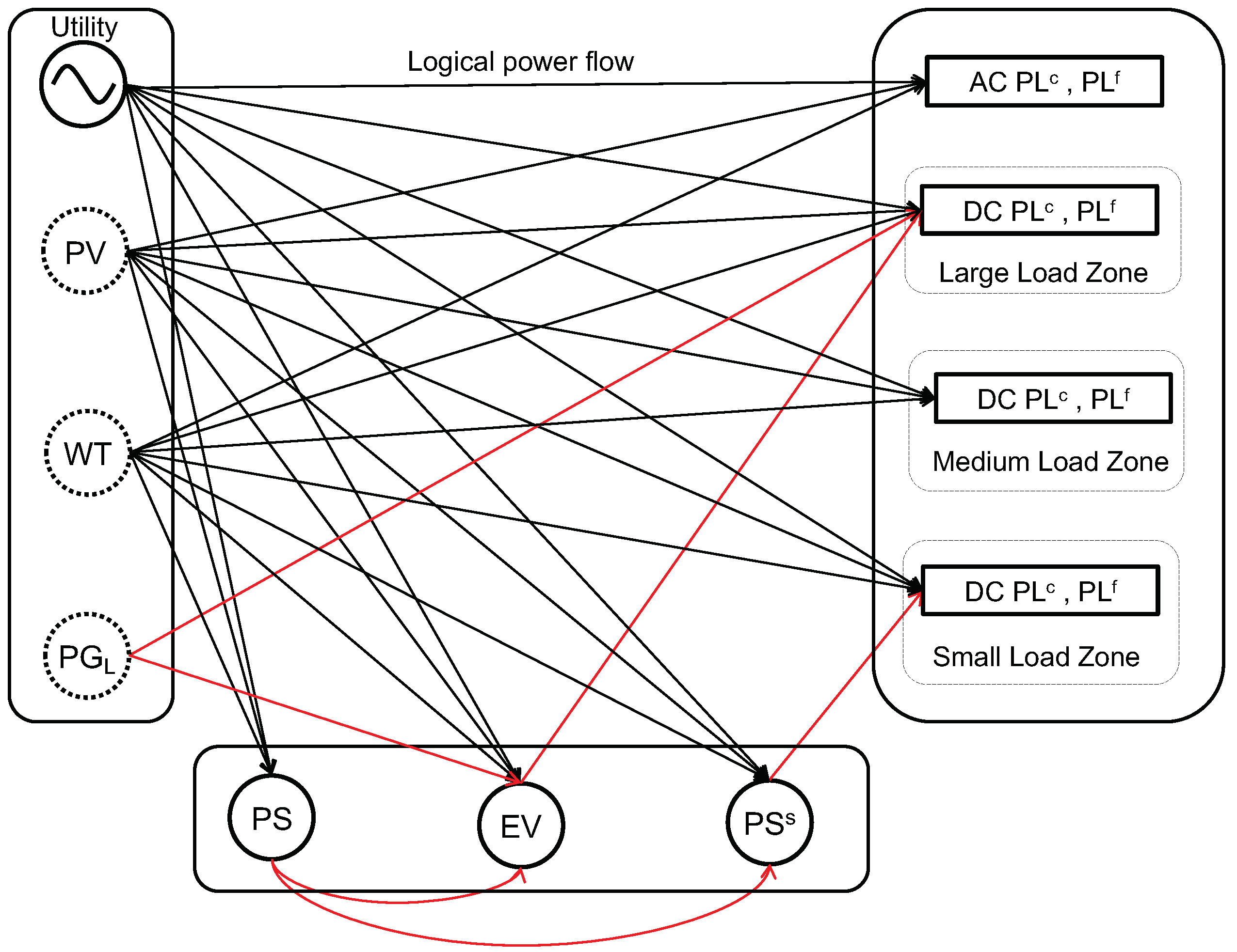
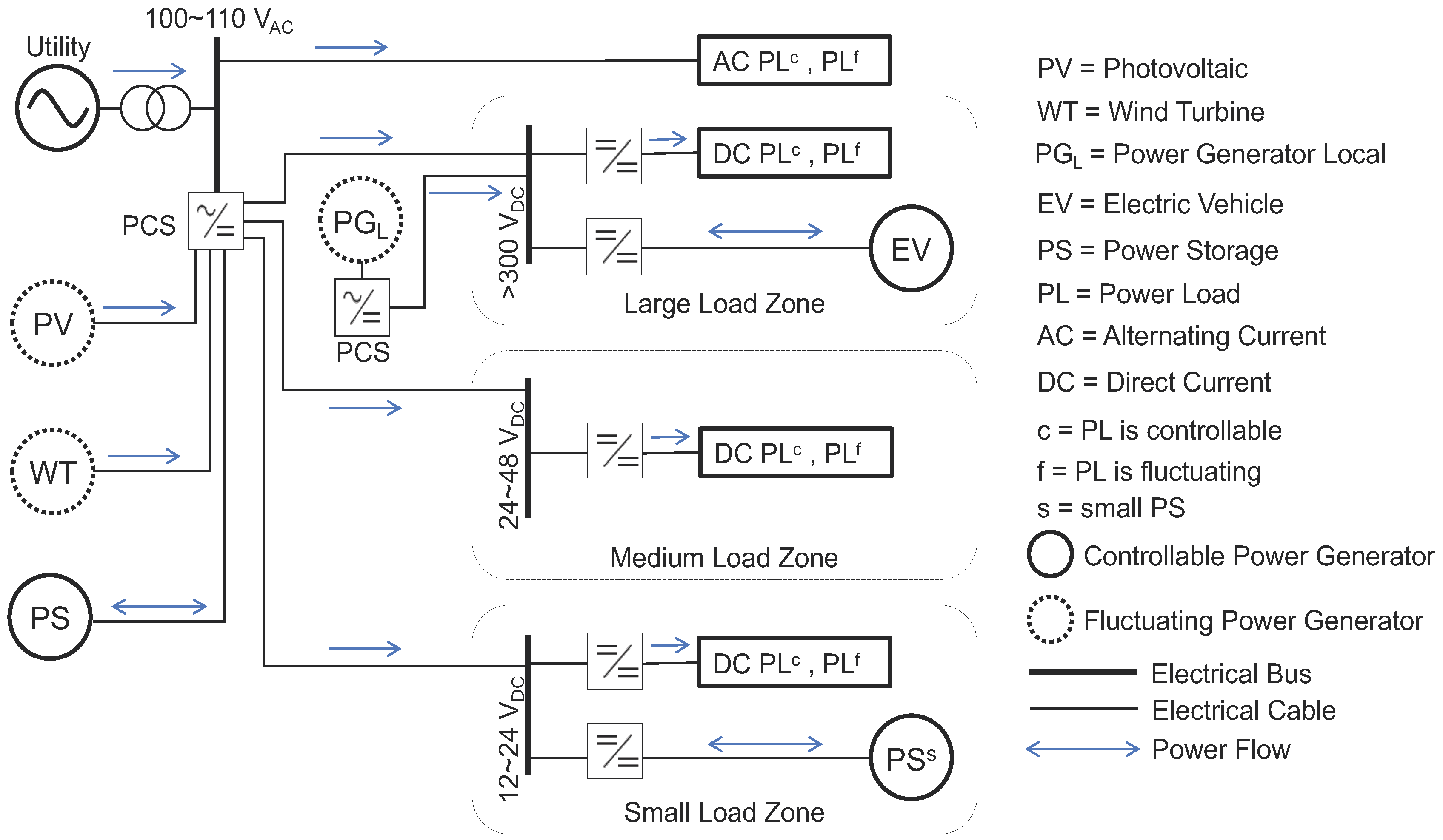
An example of such a power flow system is shown in
Figure 1. The increasing demand of integrating more DERs like photo-voltaic, wind turbines, electric vehicles, and storage systems together with power loads of both types (i.e., AC and DC) has gained much attention nowadays. Compared with a conventional AC power distribution network, the benefits of an AC-DC power distribution network are numerous. For example, a lot of power converters are required for the AC power distribution network to supply/consume power to/from DC loads/generators. The term power conditioning system (PCS) in this figure refers to the power devices that are used to convert electric power between DC and AC. All power generators, loads and storage devices are already connected to the grid through PCSs to provide the relevant interface to the type of connected device.
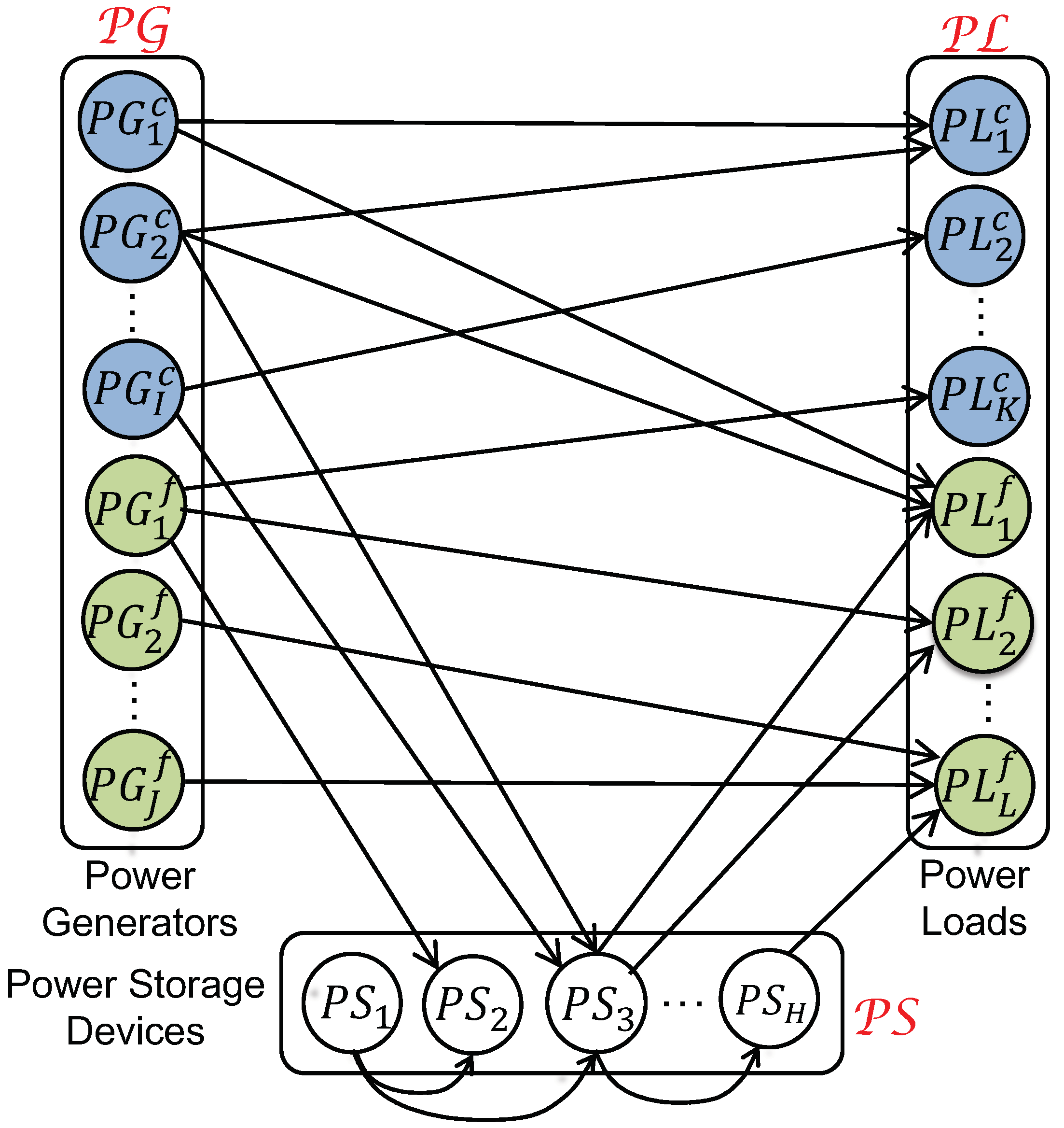
The power flow system given in
Figure 1 can be shown in the form of a graph representation as shown in
Figure 2. This shows an incomplete graph model with logical power flows (i.e., connections). In this paper, the mixture of controllable power devices and storage devices is used to ensure the minimum storage capacity required for a given power system. Through the mixture of power devices, controllable power devices will coordinate with storage devices in which the burden on the storage devices can be reduced. In this paper, the mixture of controllable power devices and storage devices is used to ensure the minimum storage capacity required for a given power system. To reduce the effects of power fluctuations triggered by fluctuating power generators and loads, a power flow assignment is required [
12,
13,
14]. This power flow assignment assigns power levels to controllable power generators, loads, and connections between power devices while maintaining the physical power constraints of power devices.
In our previous research work [
14], system characterization conditions were proposed for power flow assignment. In the previous paper, the power system consisted of fluctuating power devices (i.e., power generators and loads) and power storage devices. The study on controllable generators and loads was kept as future work at that time. To mitigate the effects of power fluctuations caused by fluctuating power generators and loads, a power flow assignment is introduced. The ultimate goal of this proposed power flow assignment is to find the power levels for all connections among power devices while keeping the power constraints. The goals of the proposed power flow assignment are, (i) the power consumption of power loads is completely satisfied as demanded, (ii) intermittent power generation is consumed fully by power loads or saved/stored in storage, and (iii) the state of charge is preserved between the minimum and maximum limitation.
In this particular paper, a more general type of power flow assignment is considered, which includes controllable and fluctuating power devices, power storage devices, and connections between them. The system characterization in this paper is the extension of the previous paper using controllable power devices. As a result, we can apply proposed work to a broader system consisting of both controllable and fluctuating power devices and connections (and hence energy transfer) between storage devices.
The rest of the paper is arranged as, In
Section 2, related works have been discussed.
Section 3 shows the system model of the proposed power flow system including (i) categorization and representation of power devices, (ii) physical constraints of power devices, and (iii) power flow assignment and characterization problem. In
Section 4, a simple power flow system consisting of multiple power generators and loads of different types, multiple power storage devices, and connections among them are considered for power conservation. The proposed system characterization problem with controllable and fluctuating power devices is explained in
Section 5. In
Section 6, the demonstration for the validation of the proposed system is presented including (i) condition checking and
minimization by LP framework, (ii) theorem application and
minimization, and (iii) balancing between power storage devices and grid. Finally, in
Section 7, concluding remarks are discussed.
2. Related Works
The ever-growing penetration level of distributed energy resources (DERs) and the technological advancement of power electronics have a significant effect on the development of modern power systems. In recent years, solar and wind energy sources have attained rapid growth and development in power systems. However, energy generation from renewable energy sources is uncertain because of power fluctuations. Energy storage systems are an extremely important part of a power system. There are numerous benefits and applications of power storage devices into the power grid such as reducing peak power demand, carbon footprints, constant and reliable power supply to consumers, and power fluctuations of renewable energy sources.
The power consumption levels of electric loads need to be satisfied and for this, the power grid must be equipped with a large generation capacity. However, due to dynamic power demand fluctuations/variations, the connected power generators may not meet power consumption [
15]. The advanced information and communication systems equipped with power sensing and controlling abilities e.g., smart power sensors and power actuators, are connected to power devices for real-time power measurements, power transmission, and power control [
16,
17,
18].
The economic development of any country can be evaluated from the rate of power losses in the power system. There are many efforts on research and industrial level to reduce the power losses. According to the research reports, the power losses can be reduced by efficiently installing the power storage systems to any power system [
19,
20]. The power losses can be reduced by (i) reconfiguration of the power grid by optimal placement of the distributed sources, (ii) power balance-ability of power generators, loads, and power storage devices, and (iii) efficient utilization of renewable sources considering their power fluctuations [
21,
22].
This particular paper targets the above issues by providing the guidelines for a power system such as what should be the optimal size, placement, and capacity of a power storage system requested for any given system. It also helps to identify the physical limitation of power generators and loads that a given power system must have to continue safe operation in the presence of power fluctuations.
In [
23], a deterministic approach of an energy system is introduced which consists of power generators, loads, and storage devices. The objective of this research is to optimize supply and demand with the minimum cost of power supplied to energy. Power storage devices are used, and their charging and discharging operations are minimized to reduce power supply to loads. However, the lack of system guidelines considering the physical constraints of power generators and loads is observed. Additionally, the safe operation of the power system in the presence of power fluctuations is not discussed.
Another aspect of the integration of storage systems to any power system is the lack of clarity in planning the operation of power storage devices [
24,
25]. For example, which size of the storage is suitable and useful for the power system under consideration. The demonstration scenario in our paper can help in the planning phase of the power storage system.
Reduction in demand charges (DC) [
26] is another motivation for power storage devices. The energy storage systems can be optimized to minimize the utility charges. The consumers can get the benefit to reduce power demand from utility and give profit because of the power variations in their demand schedules (e.g., usage of power at different times).
Furthermore, some papers in the literature [
27,
28] focus on combining the PV panels with energy storage capacity for reducing demand charges. These papers consider a static limit of
as a physical limitation of power storage devices. However, the minimization of
in our paper is more practical, which can keep time-varying power generation and consumption patterns within limitations.
Our contribution is this particular paper is the extension and generalization of our previous research work with the addition of controllable power devices and connections between power storage devices. To show the effectiveness of our proposed system characterization, a couple of demonstrations are presented in this paper with different scenarios and conditions. The power flow system in this paper consists of multiple fluctuating power devices, multiple controllable power devices, multiple power storage devices, and connections that are not the complete connection between power devices as shown in the system model section. By cautiously listing the connection-oriented power flow paths of energy along the connection direction from power generators to power storages and power loads, and the connection-oriented power flow paths of energy along the counter-flow direction from power loads to power storages and power generators. For this, we estimated the state of charge () of power storages triggered by the energy imbalance between generated and consumed energy. The consideration of capacity constraints, i.e., min/max limitations of together with power fluctuations of fluctuating devices, the characterization conditions that power generators and loads must have to keep of power storages within the capacity range have been derived. These system conditions provide guidelines for a power system that can continue safe operation even in the presence of power fluctuations. That is, a feasible power flow assignment for a power flow system can handle issues such as estimation of the power storage capacity that a storage device must have, physical constraints (i.e., maximum/minimum power levels) that power generators and loads should have, and how the power flow connection should be arranged is considered.
In [
29], a SOC-based control strategy for compensating the power fluctuations from the generator side has been proposed. However, power fluctuations from the demand side are not considered. Additionally, the SOC limitations are kept through feedback control strategy only for the storage point of view. In our proposed power flow system, conditions are proposed that can keep not only the limitations of storage battery, but also the overall system with generators, loads, and connections between them. The proposed conditions can provide the safe operation of the whole power flow system not only for storage devices.
In [
30], the authors analyzed 240-bus using a MILP method to compute the optimal location and sizing, and power and energy rating of storage devices. The integration of renewable energy resources penetration is improved using storage devices while reducing the renewable curtailment on the power network. However, the physical constraints of power generators and consumers, and connections arrangement between power devices were not considered. This overlooks the potential of power device constraints at the device level as well as transmission level.
3. System Model
This section shows the details of a power flow system that is considered in this particular paper along with power flow assignment problem to keep balance between fluctuating power levels of fluctuating power generators and loads by controlling power levels of controllable power generators, loads and power storage devices. The system characterization is also explained in this section.
3.1. Categorization and Representation of Power Devices and Connections
The power flow system considered in this paper is comprised of distributed generators, several loads, power storages, and connections (i.e., power flows) that connect devices. A power generation device provides electricity to power loads and power storage devices. A power load is an electric device that consumes electricity supplied by power generators and/or power storage devices. A power storage device can store (i.e., charge) energy when power generators generate excessive power or supply power (i.e., discharge) to power loads when the power supply is not enough. We did not consider any specific type of power generator. As for the characterization of each generator, we consider the minimum and maximum power levels of power generators known as physical constraints and also time-varying power generation levels of power generators. Schematically,
Figure 3 depicts the generalized system model. Two different types of power generators and loads are considered considering their types as controllable and uncontrollable. A controllable power device (i.e., generator/load) has the ability to control its power, precisely. These controllable power devices can supply and/or absorb power to mitigate the effects of power fluctuations caused by uncontrollable power devices. However, an uncontrollable power device (i.e., generator/load) is not able to control its power. Throughout this paper, we use the word
fluctuating to represent
uncontrollable power devices.
Here, the power generators are indexed as, , , or without distinction between fluctuating and controllable ones, as . Where I and J show the total number of the power generators including controllable and fluctuating, respectively. Furthermore, all power consuming devices (i.e., loads) are indicated as or simply as . Where K and L show the total number of power loads including controllable and fluctuating. Similarly, storages are depicted as, , where H represents the number of storages. The sets of power generators, power loads and power storage devices in a target system are denoted as , and , respectively.
The actual time-varying power levels of power generators can be represented as and for controllable generators and fluctuating generators . The actual time-varying power levels of power loads are shown as and for and , respectively. The actual time-varying input power level and output power level for a power storage are indicated as and , respectively.
A connection or power flow can be defined as an ordered pair of power devices. As an example, a connection between a and a can be established and shown as, . Similarly, a connection can be represented between a generator and storage as , a connection can be shown as between a storage and a load , and a connection between storage and as . Each power flow (i.e., connection) is given with time-varying level of power in Watt as , , and that represent the amount of power sent from a first argument (i.e., power device) to another power device shown with the second argument on connection at time t.
3.2. Physical Constraints of Power Devices
All generators and loads have power level bounds to represent the minimum and maximum power bounds.
where,
,
,
, and
are given as minimum power limitations and
,
,
, and
are given as maximum power limitations.
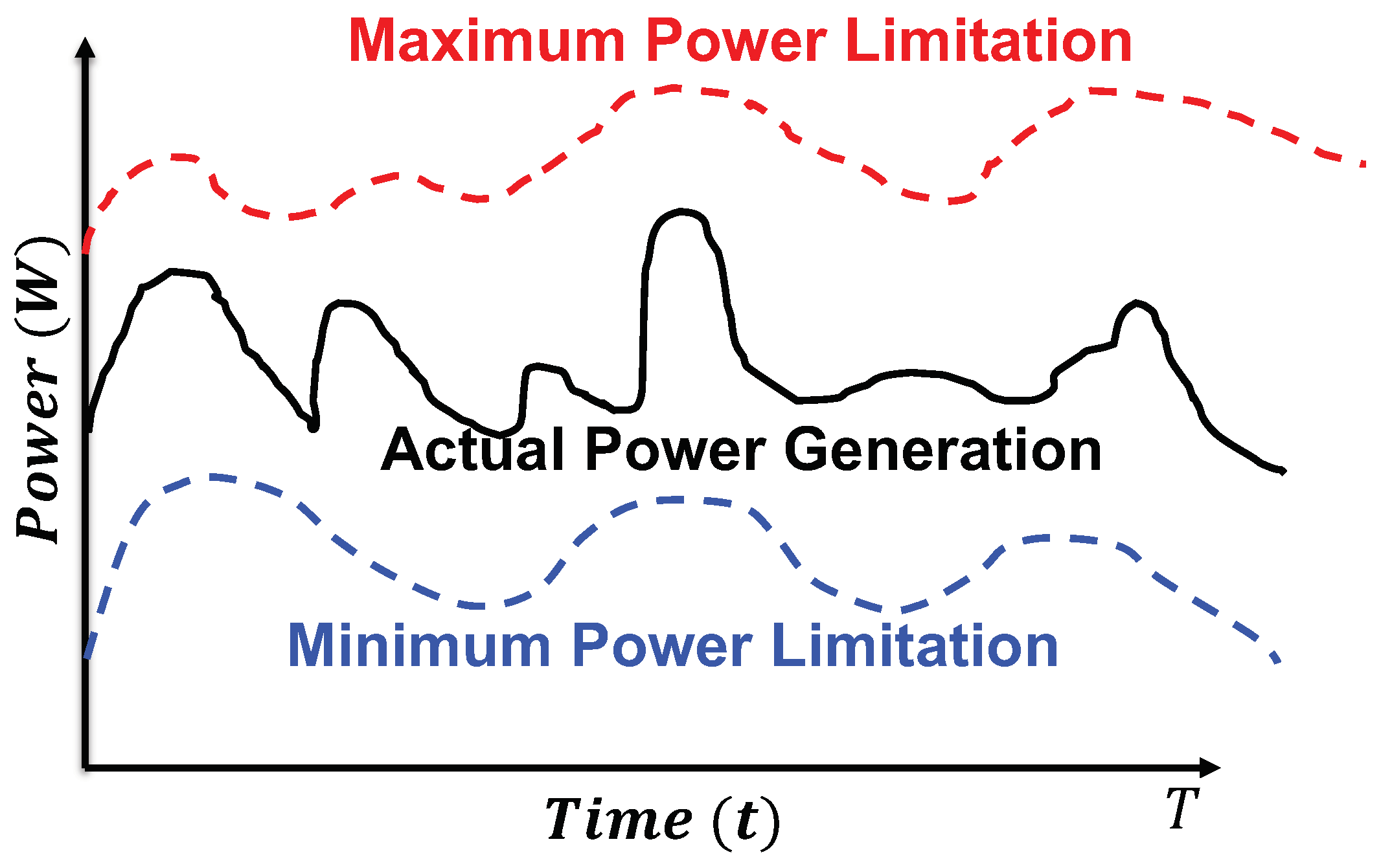
As for the power loads and power generators of fluctuating type, we consider time-dependent minimum and maximum power bounds as depicted in
Figure 4 from our previous paper [
14], which can be available from historical data of system operation, in addition to constant physical limitation as follows.
On the other hand, for a controllable power generator/load, the physical limitation is assumed to be achievable at any time, i.e., , , .
The energy levels of a generating power and energy levels of consuming power during the times from 0 to
t can be represented as
and
, accordingly.
Similarly, we will define the following.
One of the parameters of a power storage device is
, i.e., state of charge of a power storage device, which is calculated by (
11), where
and
are the charging and discharging efficiency. In addition,
is the energy storage capacity, and
is the initial state of charge of the power storage device. There are two types of definitions of SOC; one is based on the integral of current flowing in/out of the storage battery [
31,
32]. Another one is based on the integral of energy as shown in [
29,
33]. We follow the latter definition.
To avoid the forced shutdown of the storage battery due to over-discharge or overcharge of storage device,
is required to stay between a certain range given by (
12).
Moreover,
and
are also assumed to be limited as;
3.3. Power Flow Assignment and Characterization Problem
To adjust power fluctuations of fluctuating devices (i.e., loads and generators), power assignment is essential. The power assignment proposed in this paper finds power levels for controllable devices and power flows (i.e., connections) among devices while maintaining (
1) and (
3), (
12)–(
14). The ultimate goals of the proposed power flow assignment ensure that the power generated by fluctuating power generators is used by loads completely, (ii) the power demand of loads are satisfied completely, and (iii) the capacity of power storage is kept all the time (i.e., maximum and minimum limitation).
The main objective of this particular paper is not the problem that how the power assignment problem is solved rather this paper shows the structural conditions (i.e., system characterization conditions) for a system to have a feasible solution of power flow assignment. This shows that the feasible power flow assignment can consider issues such as the estimation of power storage capacity of a storage device for a power system should be, how small/large the power limitations of power generators and loads should be, and how power flow connections can be arranged. All the above issues are related to each other, therefore, the characterization conditions can represent physical constraints and capacity constraints of power devices, and also the limitation on connections between devices.
4. Energy Conservation in a Simple Power Flow System
In this section, a simple system model comprised of loads, generators, and power storage devices is discussed, and a system characterization for safe operation under fluctuations, which will be discussed in depth later, is demonstrated.
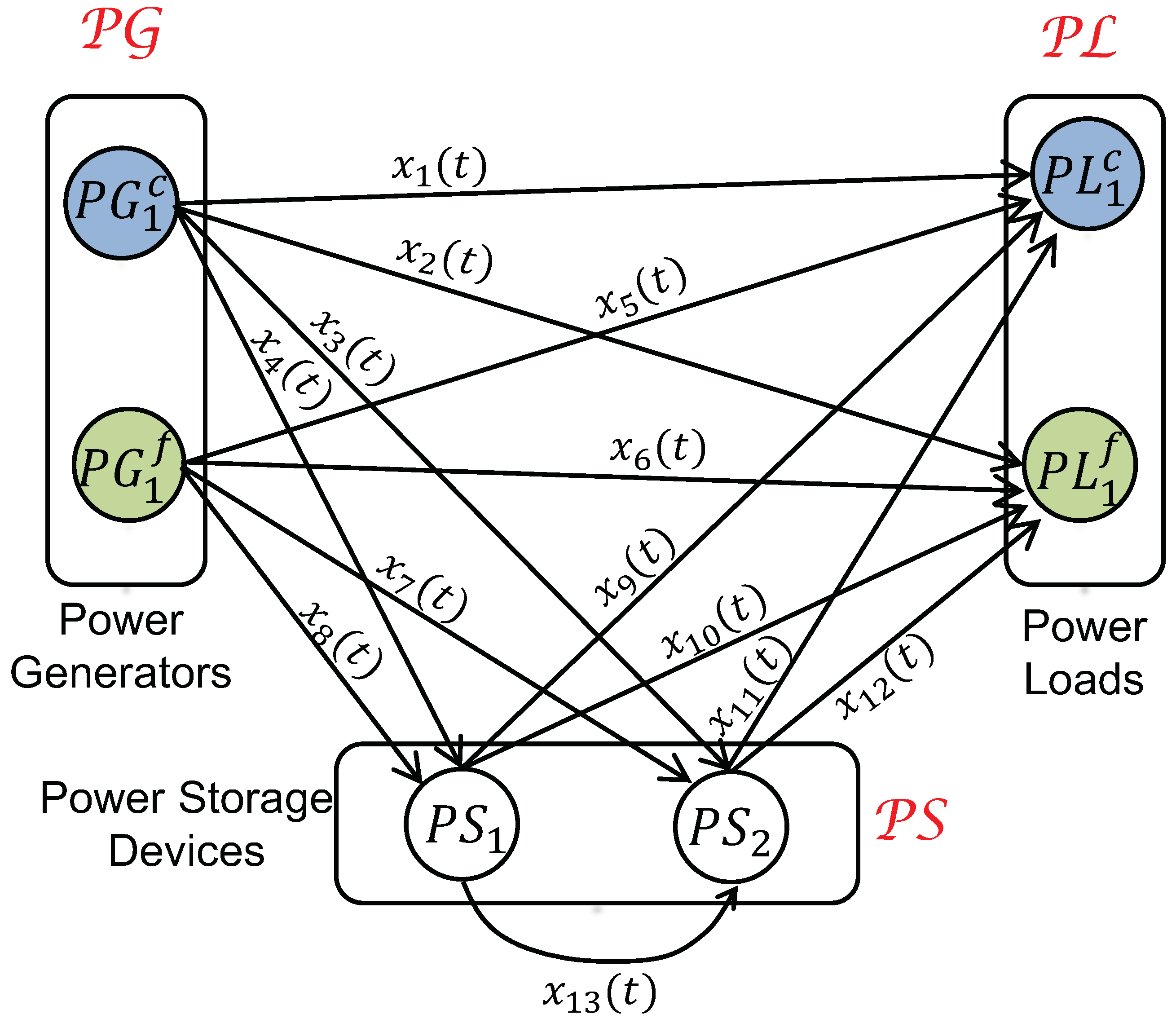
There are two power generators of different types; controllable power generator,
, and fluctuating power generator,
. Similarly, there are two power loads of different type; controllable
and fluctuating
. Along with generators and loads, two power storages and connections among power devices are in the basic system model as depicted in
Figure 5.
The proposed power flow assignment introduced in this paper identifies power levels for connections between power devices (i.e., , , ), and power levels for controllable generator and load, i.e., , based on given power levels of fluctuating generator and load and , .
The power levels on connections
,
,
, and
can make the total instantaneous power generation
at any time
t of controllable power generator
, which can be represented as,
In the energy levels, it can be shown as,
Similarly, for the other power generators and power loads, we have the following,
and,
and,
The state of charge of storage
in an ideal lossless case, where
can be shown as,
Similarly, the state of charge
of storage device can be represented as,
Total stored energy of two power storage devices can be shown as,
In other words, it can be written as,
Because of the
limitation (
12) of power storages, we have
Using (
15), the difference between consumed and generated energy by loads and generators must be bounded as follows,
These limitations are requested to hold even in the worst case. With respect to the first inequality, the difference between consumed and generated energy becomes minimum when
and
, which, in turn, can be maximized by the help of the controllable generator and load by choosing
and
. As a result, we have the first condition as;
Similarly, as for the second inequality, the difference between consumed and generated energy becomes maximum when
and
, which can be minimized with the help of the controllable generator and load by choosing
and
. Therefore, the following second condition can be derived.
This is the case that applies to a system comprising of limited power loads, generators, power storages, and the connections among them. However, the characterization conditions for a complex power system comprised of multiple generators and loads of both types, power storages, and connections among devices are critical and challenging tasks.
5. System Characterization
5.1. Main Theorem
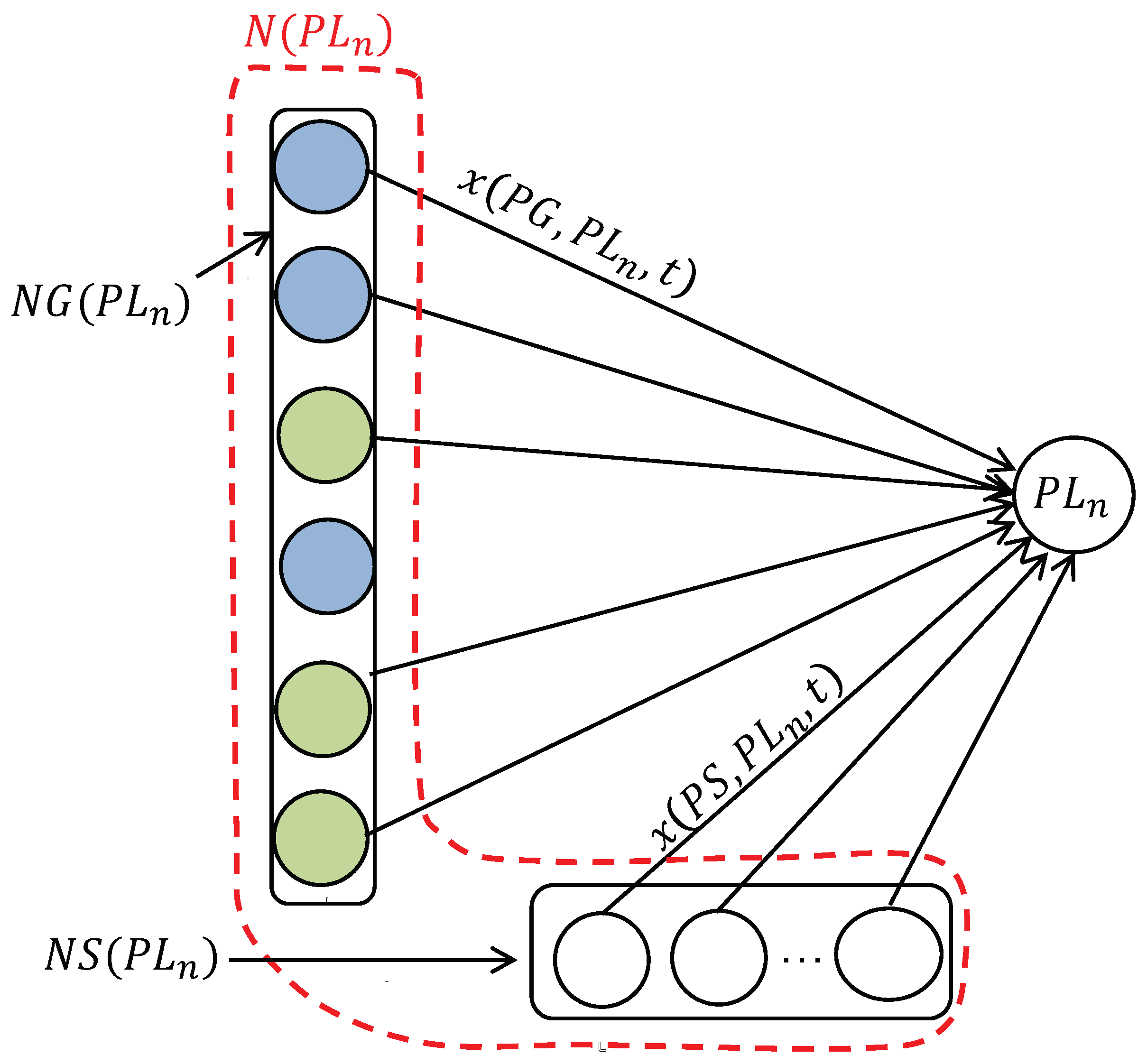
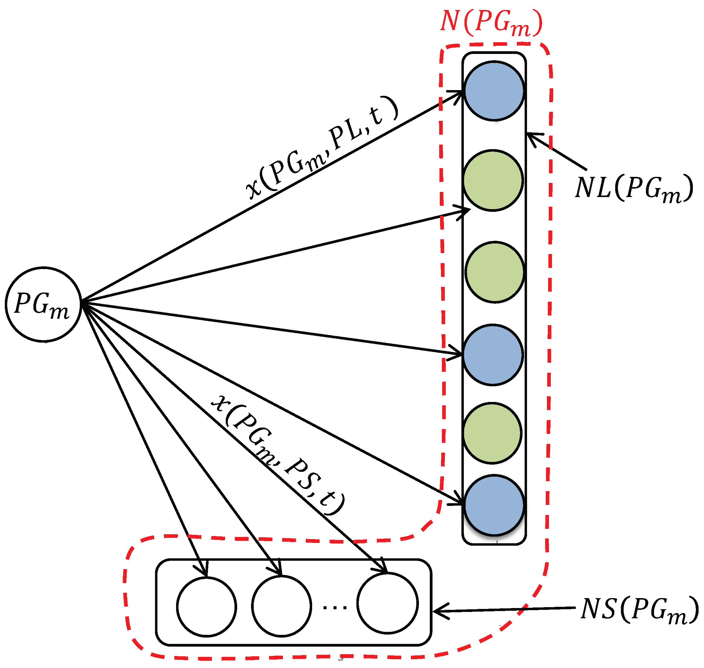
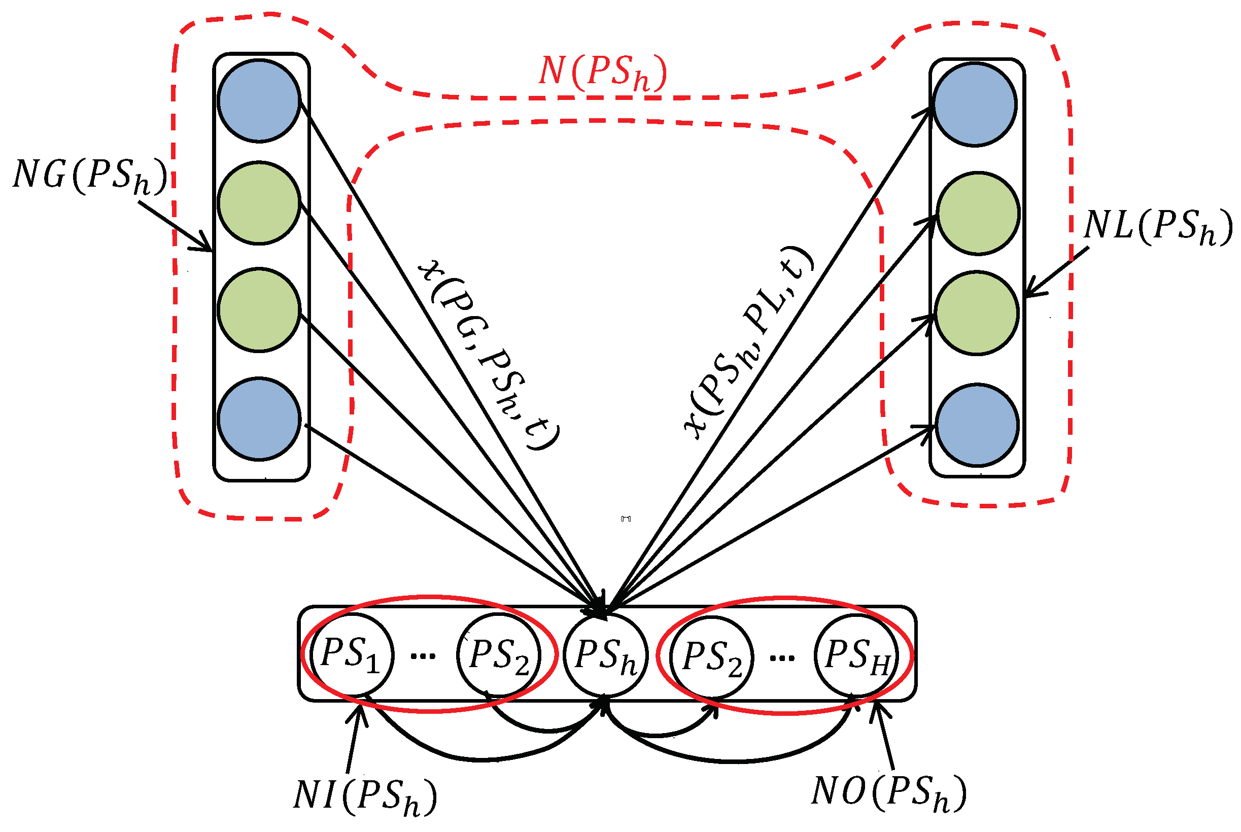
By considering the graph model as shown in
Figure 3, when a connection
is available for power transfer,
is specified as a neighbor of
and vice versa.
The set of neighbors of a device is denoted as .
When
is a set
of devices,
is the union of
,
. This is further divided into three sets of neighbors as
,
and
depending on the type of neighbors, see
Figure 6,
Figure 7 and
Figure 8.
Furthermore, to show the neighboring sets of power storage devices,
and
are used to represent incoming and outgoing neighboring sets of power storage
, see
Figure 8 for representation of neighbors.
As an extended result for characterizing a system with storage devices to have a feasible power flow assignment and as the main contribution of this paper as well, the following Theorem 1 is submitted.
Theorem 1. If the power flow assignment problem has a feasible solution, then the following two characterization conditions for a power flow system are satisfied.
Condition 1-1:, Condition 1-2: , 5.2. Necessity Proof of the Theorem
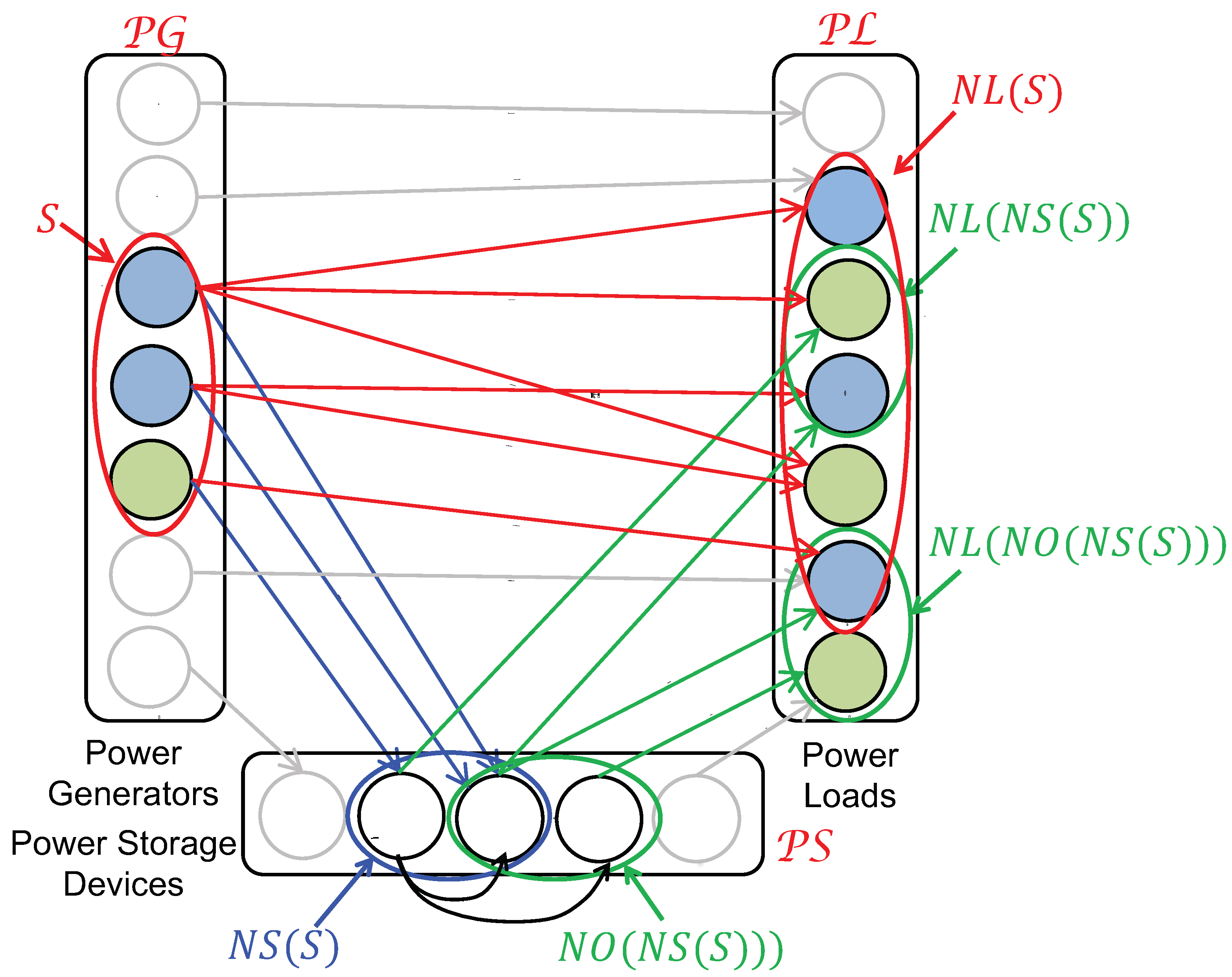
Proof of Theorem 1. Let
S be any subset of generators of
, the total power generation by mixture of generators (i.e., controllable and fluctuating power generators) existing in subset
S is partly used by mixture of power loads in
and partially saved in storage devices in
. This shows that power sent directly from power generators in
S to power loads in
and some indirect power transfer to power loads in
and
via storages in
and
(please see
Figure 9).
However, the set of power loads in
and set of power storage devices in
may receive power from other power generators outside
S. Similarly,
can receive power from power generator outside
S and from storage devices outside
, the set of power loads in
and
can also receive power from other power storage devices not in
and
. Therefore, the total sum of power consumption consumed by power loads in
and the increase of energy in storage devices in
is no smaller than the total generated power by power generators in
S. From this point of view, we can conclude that
In order to keep maximum storage capacity limitation
, it can be written as,
By considering the worst-case scenario for fluctuating power devices and maximum cooperation of controllable power devices, the above can be shown as,
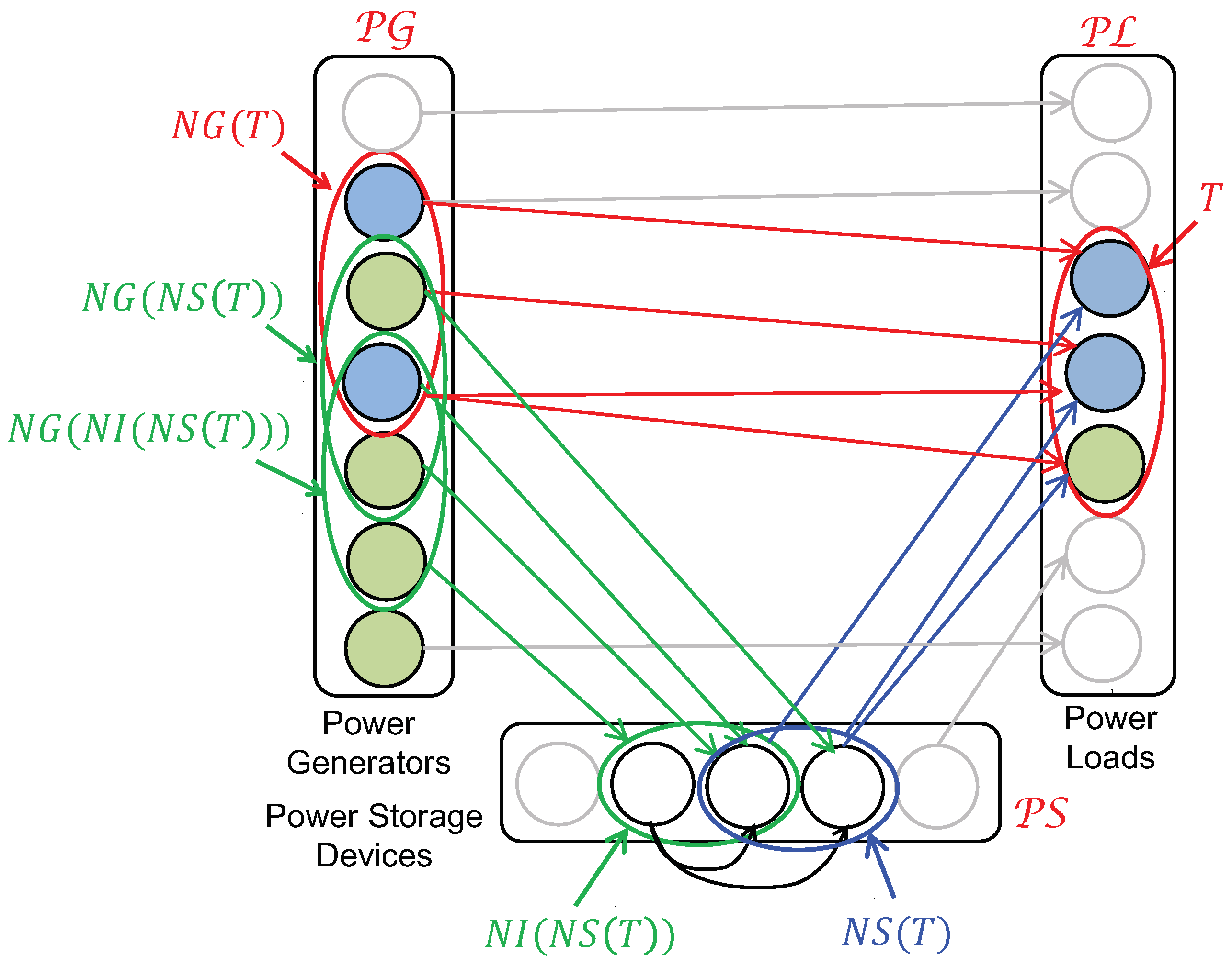
On the other hand, when we consider any subset
T of
, the total energy consumed by power loads in
T is provided only from power generators in
(the energy is directly sent to
T), power generators in
and
(the energy is once sent to storage devices in
and
and then be conveyed to
T with/without time delay), and storage devices in
(see
Figure 10). Note that the storage originated energy is only the initially stored energy, and the part of storage originated energy that is sent to
T is measured as the decrease of stored energy from the initially stored energy. Since power generators in
may provide energy to other storage devices outside
and other power loads outside
T, and storage devices in
may provide energy to other power loads outside
T, the total consumed energy by power loads in
T is no larger than the sum of the energy generated by power generators in
and the decreases of stored energy from initial states of storage devices in
. From the above observation, we have,
In order to keep minimum storage capacity limitation
, it can be written as,
The worst-case scenario for fluctuating power devices and compensation of controllable power devices can be represented as,
□
6. Demonstration
This section shows the validation and application of the proposed system characterization conditions. After a brief overview of condition checking and minimization by computer software, sections are provided as (i) Theorem application and minimization, and (ii) Balancing between power storage devices and grid.
In the first demonstration, proposed conditions (i.e., condition 1-1 and condition 1-2) are examined under different situations of the power flow system. It discusses the minimization of storage capacity using the Linear Programming (LP) framework to a given power flow system to verify whether an optimum feasible solution exists or not.
In the second demonstration, a balancing between storage devices and the energy from a grid in the environment of local area renewable energy sources is discussed through the viewpoint of our proposed theorem.
6.1. Condition Checking and Minimization by LP Framework
Based on our theorem, we have implemented computer software for condition checking and
minimization. Time-discretization has been introduced for making these problems tractable by a digital computer. After the introduction of time-discretization and the replacement of a continuous-time integral with a discrete-time summation, the condition checking can be reduced to a set of algebraic inequality checking, and
minimization can be reduced to a Linear Programming problem which is solvable using a commercial/public software tool. Now, let
be the discrete time with the normalized time interval 1. The continuous-time integral is approximated with (Sampled rectangle rule) with the summation of the sampled values as,
for
,
, and
. With respect to the condition checking, given all the information about the system, which includes
,
,
,
,
,
, etc., we will check the inequality (16) for each subset
S of
and (17) for each subset
T of
, both for each discrete time
. On the other hand, in the linear programming based
minimization, the same set of inequalities are formulated as inequality constraints with specifying
as unknown variables, and the total
, i.e.,
, is set as the objective function to be minimized.
In our practical implementation, Matlab is used for generating a LP problem instance from a given system description, and solving it. In order to prepare simulation environment, a PC with following details is used; Model: MacBook Air, Processor: Dual-Core Intel Core i5, Processor speed: 1.6 GHz, and Memory: 64 GB.
6.2. Theorem Application and Minimization
In the first demonstration, proposed conditions (i.e., condition 1-1 and condition 1-2) are examined under different situations of the power flow system. This section also discusses the minimization of storage capacity using the Linear Programming (LP) framework. The proposed theorem is applied several times to a given power flow system to verify whether condition 1-1 and condition 1-2 are satisfied or not.
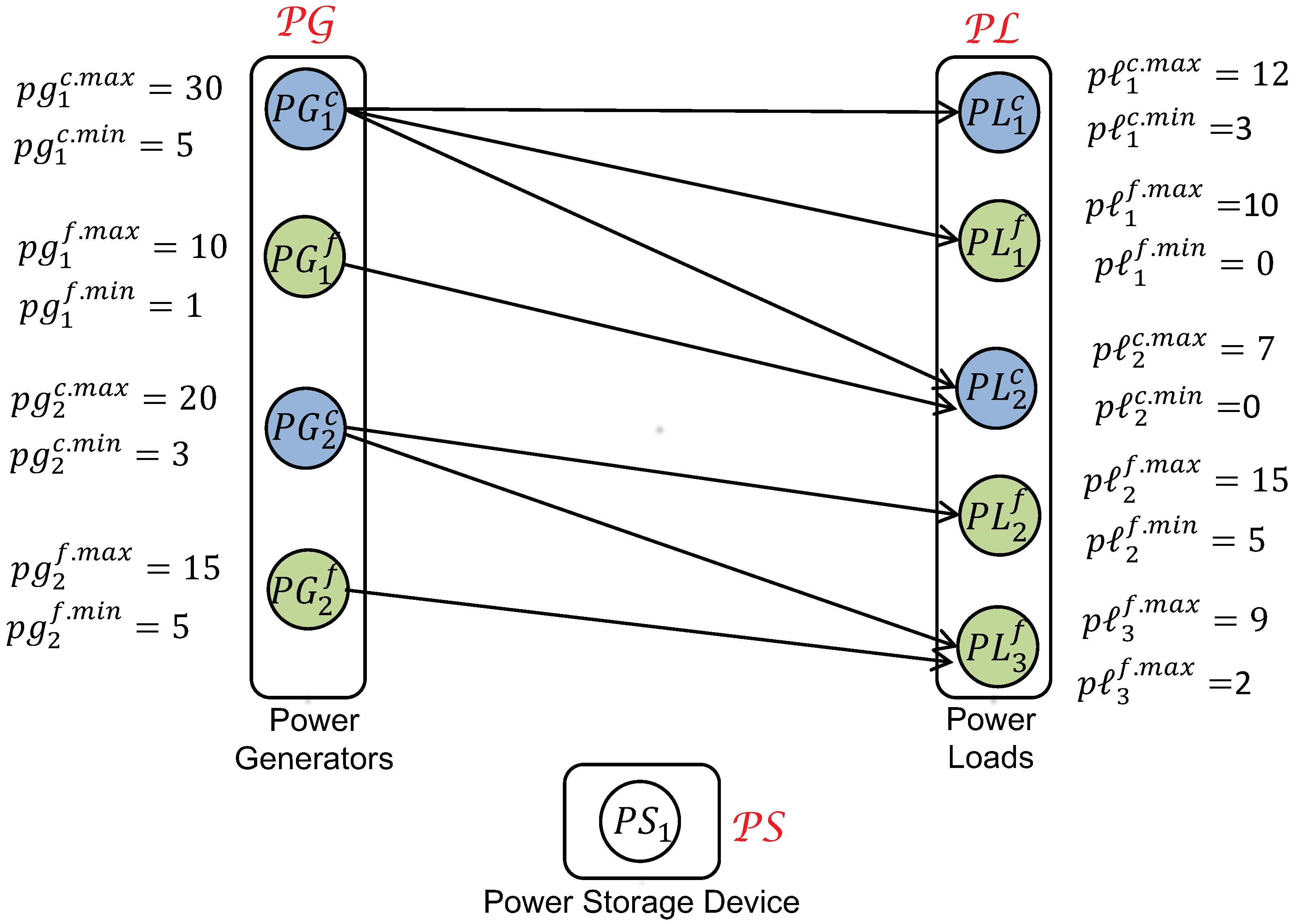
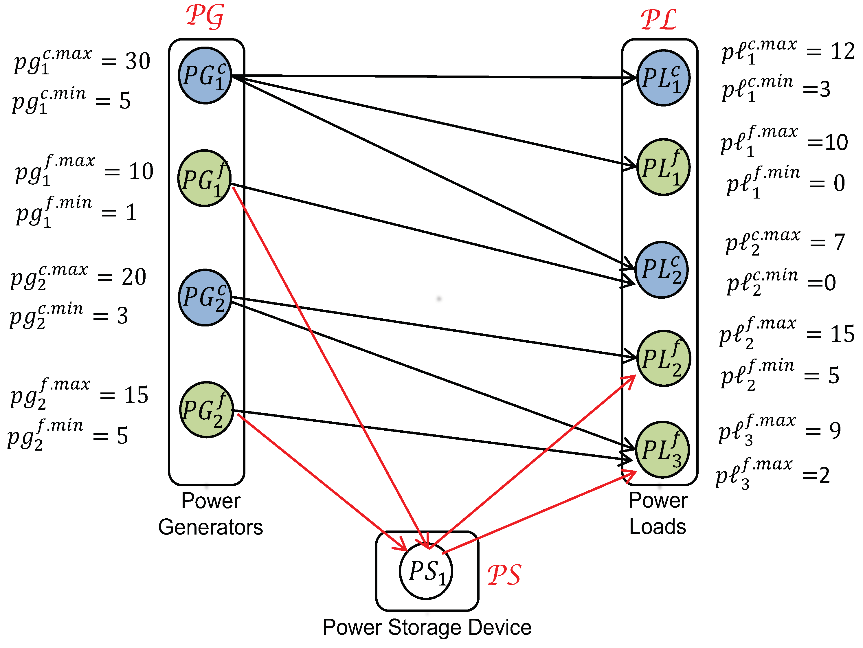
For this purpose, a demonstration system is considered which consists of four power generators, five power consumers, one power storage device, and connections between them (see
Figure 11 for the representation of the demonstration system). Two power generators are selected as controllable
,
and two power generators are selected as fluctuating
,
. As for the power consumers (i.e., loads) three of the five consumers are selected as fluctuating
,
,
, and remaining two are selected as controllable
,
.
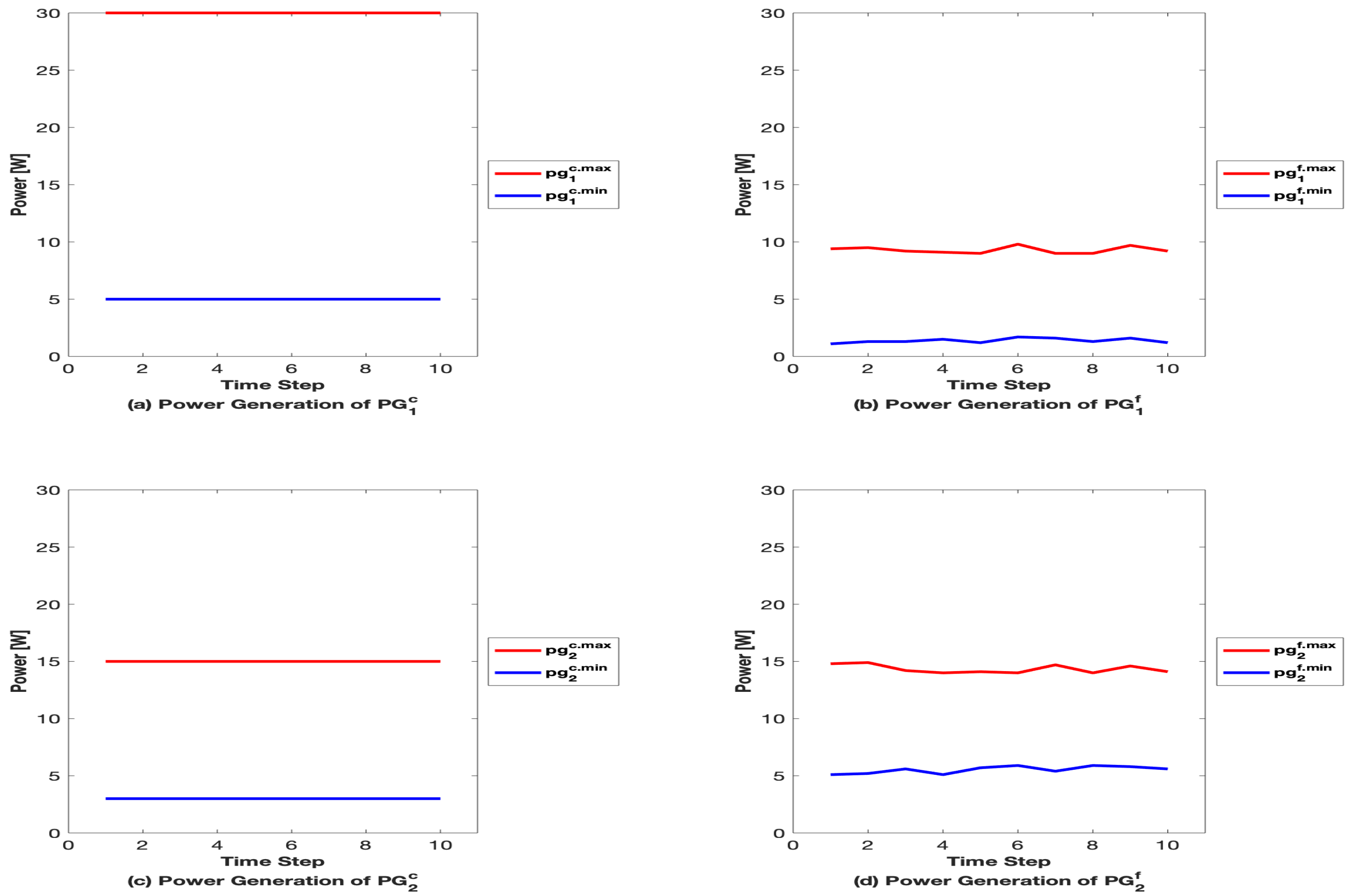
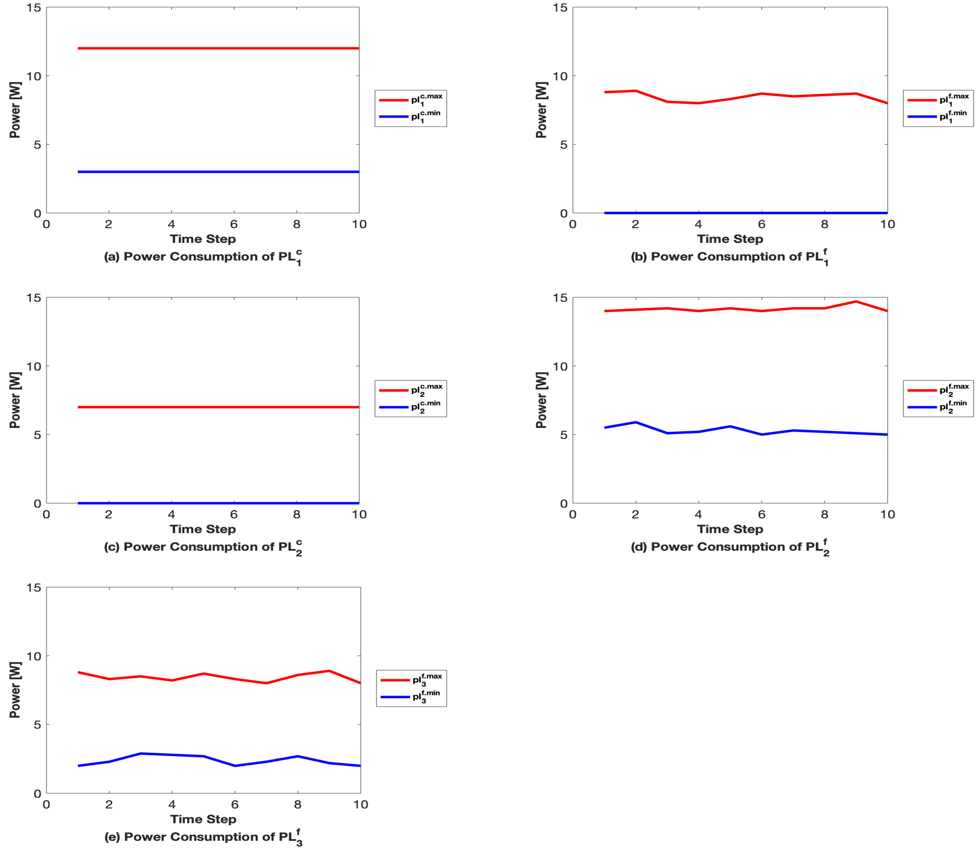
The power generation and consumption of power generators and consumers of both types are bounded between the minimum and maximum physical power constraints which are also shown in
Figure 11. To represent the power variations of the actual power of fluctuating power devices, the power generation and consumption patterns are considered as shown in the
Figure 12 and
Figure 13. The upper and lower power levels for controllable power generators and loads are set as given in
Figure 11.
At first, we apply the case when all connections to/from the power storage device are not available. That is, there is no power transfer to/from a power storage device and other power devices such as power generators and power loads. This means that the excess power of power generators cannot be stored in power storage, and power loads cannot receive power from storage devices. As a result, based on the given system, there is no feasible solution received from the LP solver, i.e., condition 1-1 and condition 1-2 are not satisfied. This shows that the storage device must be installed for the above system so that the not satisfied cases can be satisfied and to find a feasible solution for the storage device.
Now, the connections between the power storage device and power generators are added, i.e., connections from
and
to
are added from the power generation side. Similarly, connections from
to
and
are introduced as shown in
Figure 14. The given power system uses only one power storage device with
,
, and
and try to minimize
as much as possible.
Based on this system, the LP solver is applied to find the minimum capacity of the power storage, and check what happens when the capacity is smaller than the minimum solution. As a result, the minimum capacity is obtained as kWh, and we found that the condition 1-1 with subset S of the , fails when is smaller than 215.0 kWh. It can be interpreted to mean that, when is smaller than 215.0 kWh, the total energy generated by , and exceeds the energy consumed/stored by loads/storage devices connecting to these power generators. Hence, our possible choice is to use kWh, or to arrange the connection so that the excess energy can be consumed by another controllable load, which may contribute to reduce .
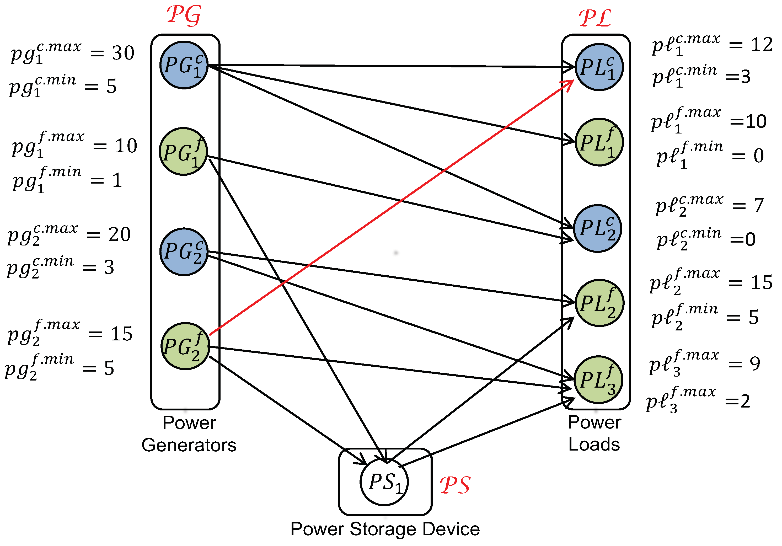
In order to satisfy the case of subset
, if we take the latter choice, and a connection from
to
is newly added to the power system, a new system is obtained as shown in
Figure 15. After applying the LP solver again to this new given power system, condition 1-1 and condition 1-2 are satisfied for all time steps, and the required capacity for the power storage device is obtained as
kWh.
The above scenario shows that the proposed theorem is used several times to find a feasible solution. The addition of a power storage device can surely eliminate the cases when conditions are not satisfied. That is, the power storage device is an essential part of any power flow system to avoid the situations when the excess of power generation can be saved in the storage device to use later and power consumption can be satisfied fully with storage device when generation alone is not enough to satisfy the demand of power loads.
Moreover, the initial solution for the system given in
Figure 14 gave the solution with a much higher capacity level, i.e.,
kWh. By adding a new connection as shown in
Figure 15 and using the proposed theorem, the capacity of the storage device is reduced to
kWh. This shows that the addition of one connection can eliminate the unsatisfied cases and also reduce storage capacity.
6.3. Balancing between Power Storage Devices and Grid
In this second demonstration, a balancing between storage devices and the energy from a grid in the environment of local area renewable energy sources is discussed through the viewpoint of our proposed theorem.
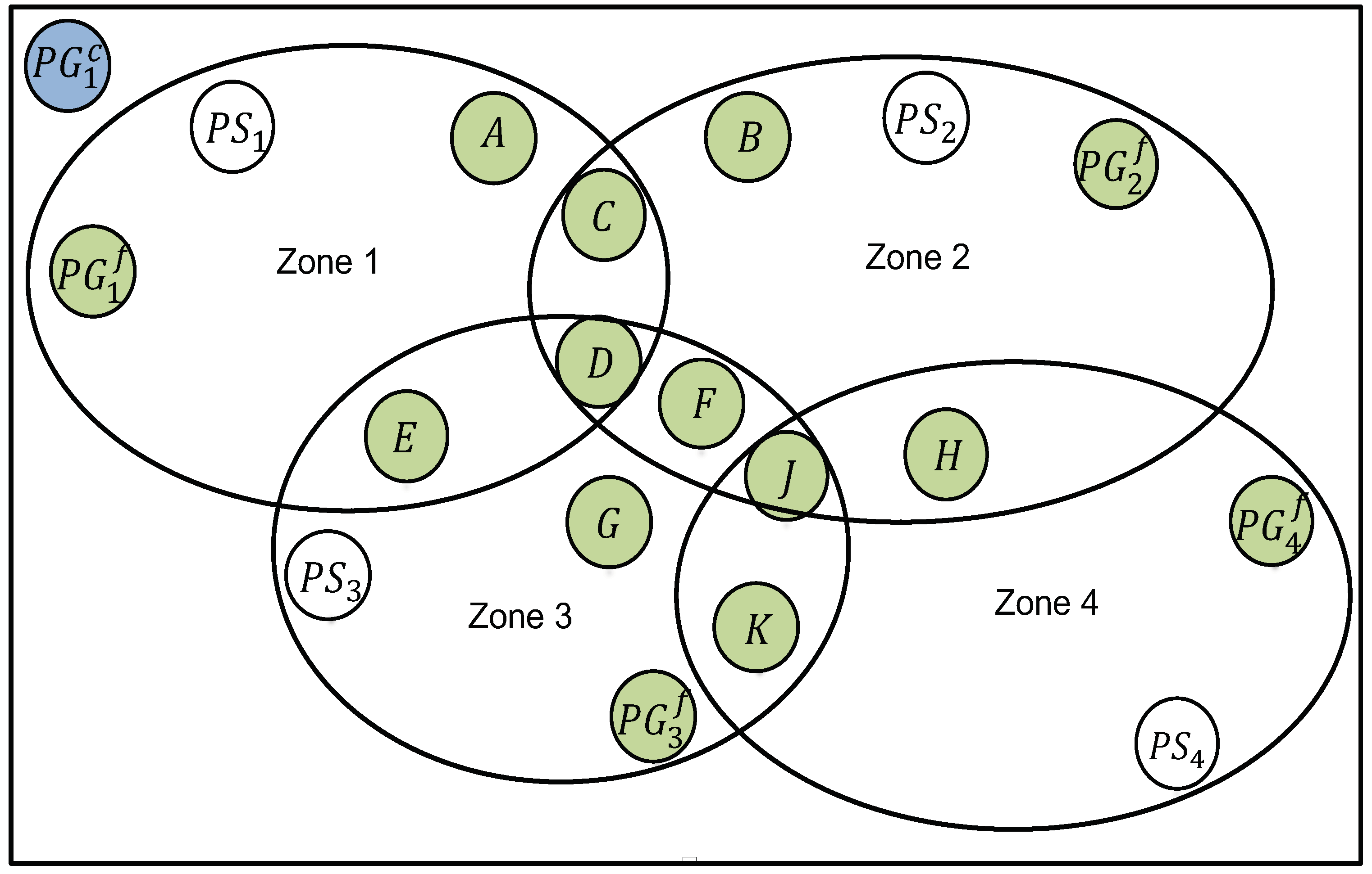
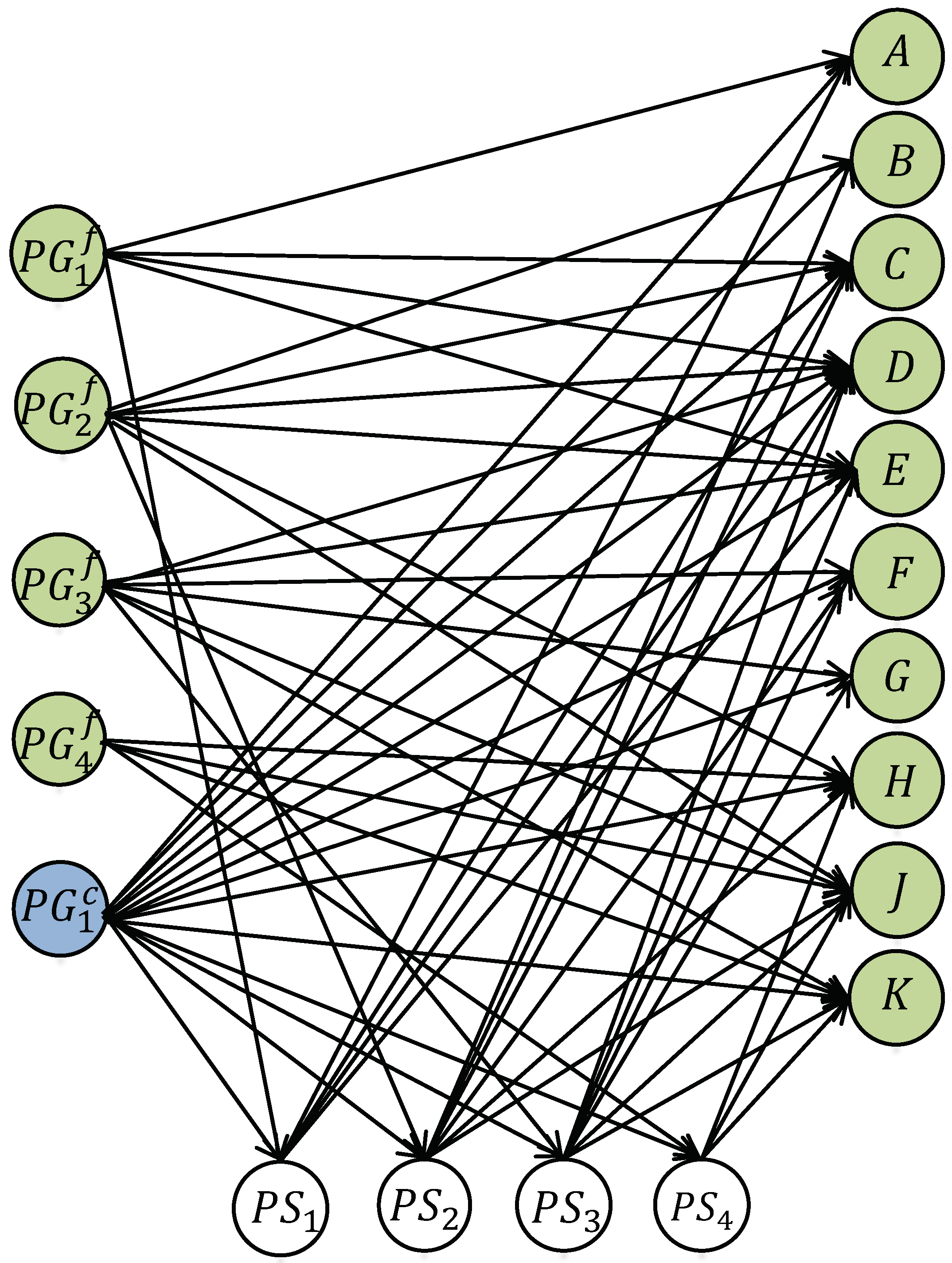
Figure 16 shows our demonstration environment, which consists of renewable energy sources (fluctuating generators), consumers (fluctuating loads) and a power grid. Each renewable energy source forms a service zone, and consumers in a zone can receive energy from a renewable energy source in the same zone. A consumer belonging to multiple zones can receive energy from multiple renewable energy sources in these zones. Besides renewable energy sources, all the members in this environment are covered under the service of an external grid. Due to the fluctuation of generating energy of renewable energy sources and consuming energy of consumers, the degree of dependence on the external grid is high. In order to mitigate this situation and to increase the degree of independency from the grid, we plan to introduce energy storage devices to this environment, e.g., one storage device to each zone.
The graph model for this environment can be shown in
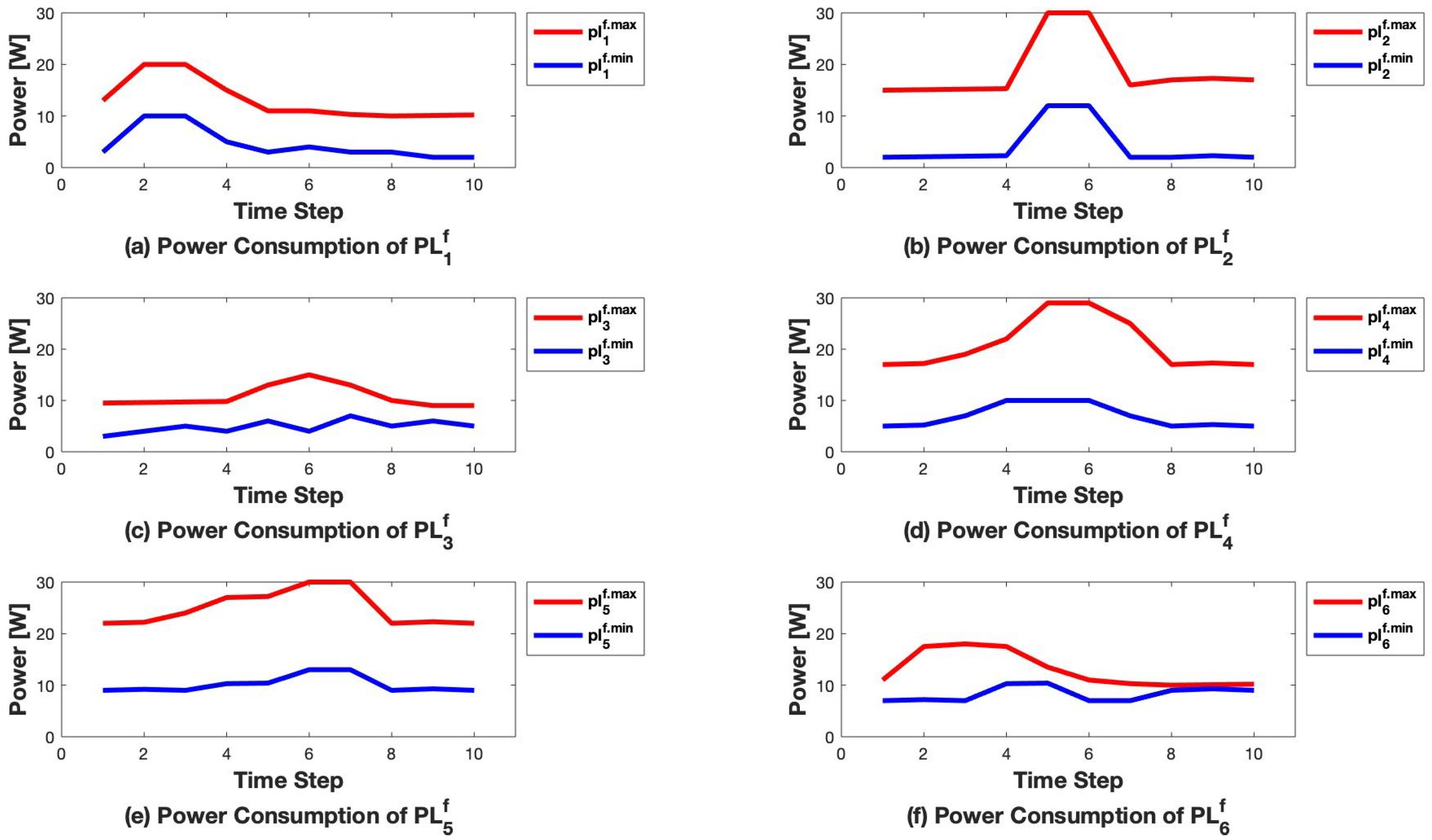
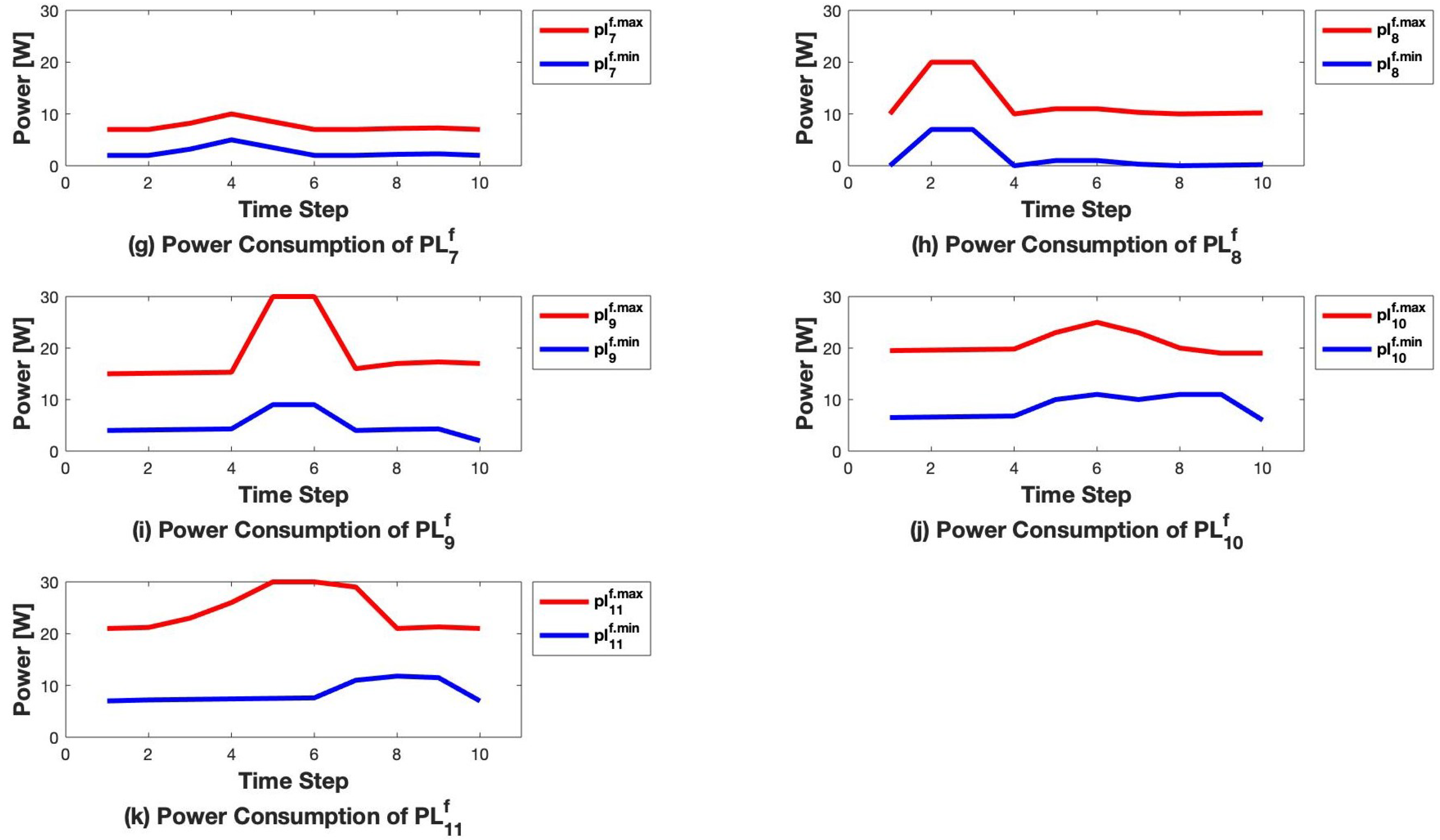
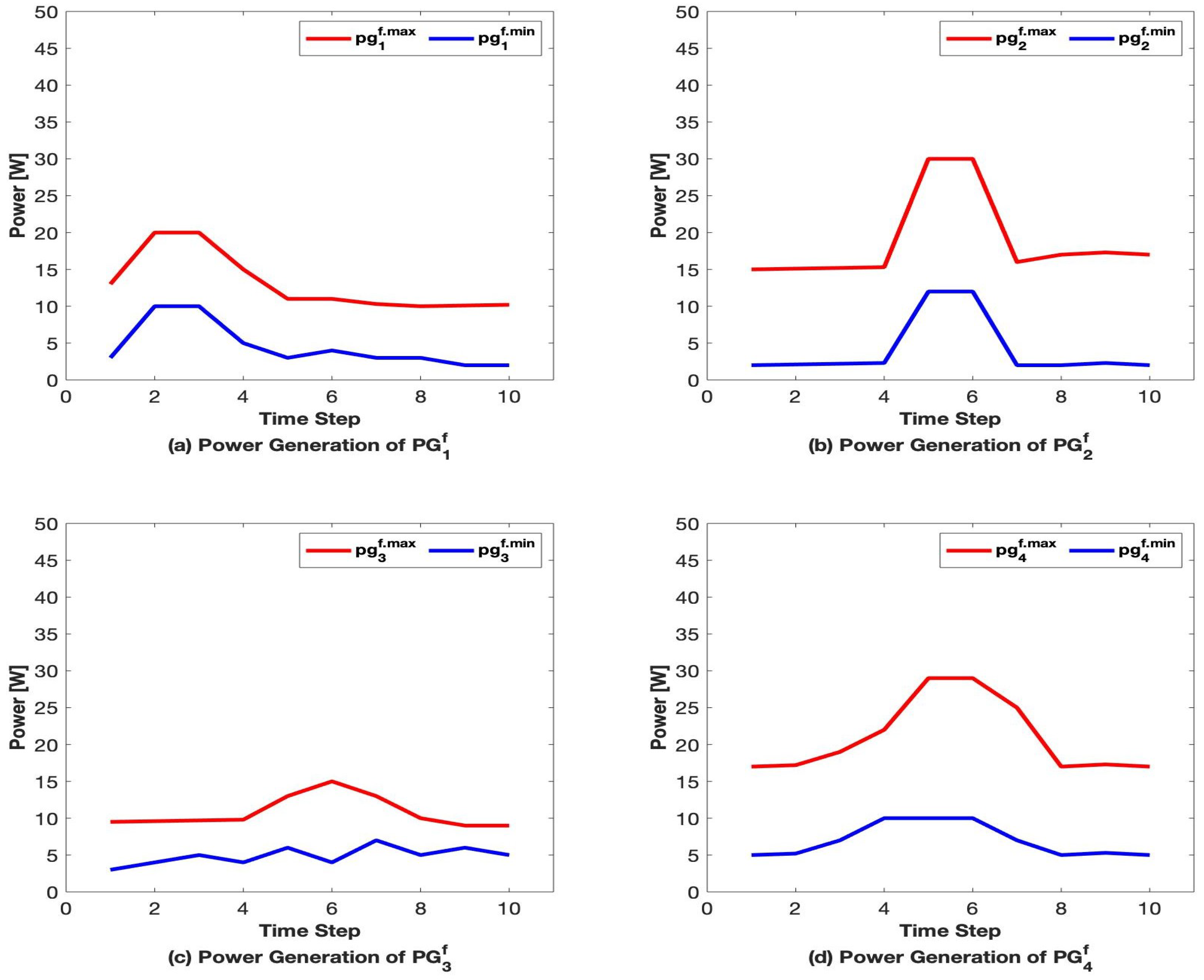
Figure 17. In addition, from the preliminary survey, we have the information about the time varying minimum and maximum power levels of each renewable energy source and power consumption of each consumer in one service term, which are shown in
Figure 18 and
Figure 19. The service term is assumed to repeat forever. Our analysis has been conducted with the following settings.
At the beginning of each service term, for every storage device is set at 0.5.
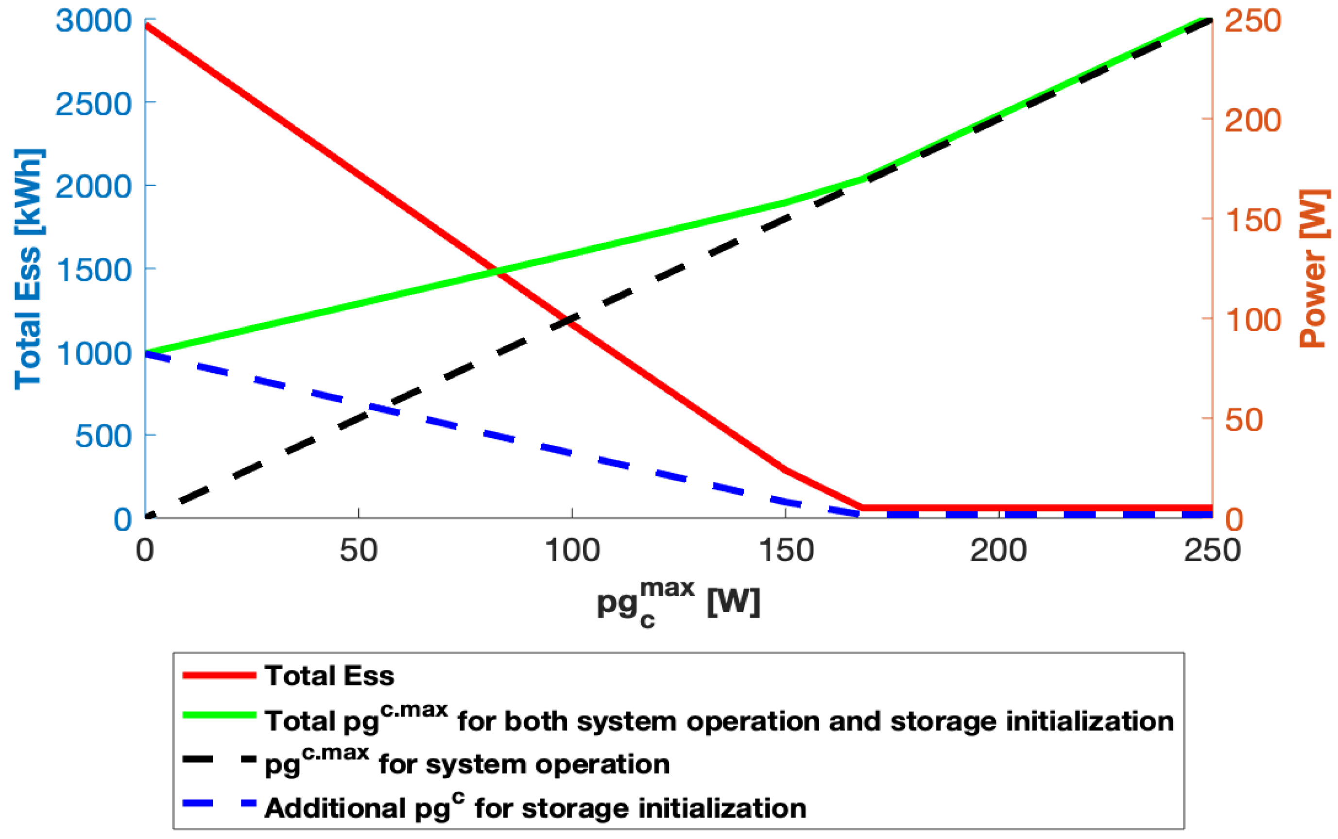
The role of the grid will be divided into two parts, one is for supporting the system within each service term, and the other for additional charging of storage devices only for setting at the beginning of each service term. With respect to the former, we will assign and for the minimum and maximum power levels, which are taken from the grid. On the other hand, with respect to the latter, we assign the power .
We will evaluate the capacity of a storage device based on our proposed theorem using for a storage device and and for the grid.
On the other hand, the power is evaluated as the average power needed to charge up all storage devices from to , where T is the period of one service term. We do not know the exact value of , instead, we will use the estimated value. The worst case is , if our conditions 1-1 and 1-2 hold.
In the following analysis, we will compute
as;
with a parameter
.
As a whole, the maximum power from the grid is evaluated with the sum of (from (3)) and (from (4)).
Based on these settings, we have evaluated minimum
(and total maximum power of the grid) for various different setting of
(
for every case).
Table 1, all numerical entries are rounded to one decimal place, like 154.08 → 154.1, 82.340556 → 82.3.
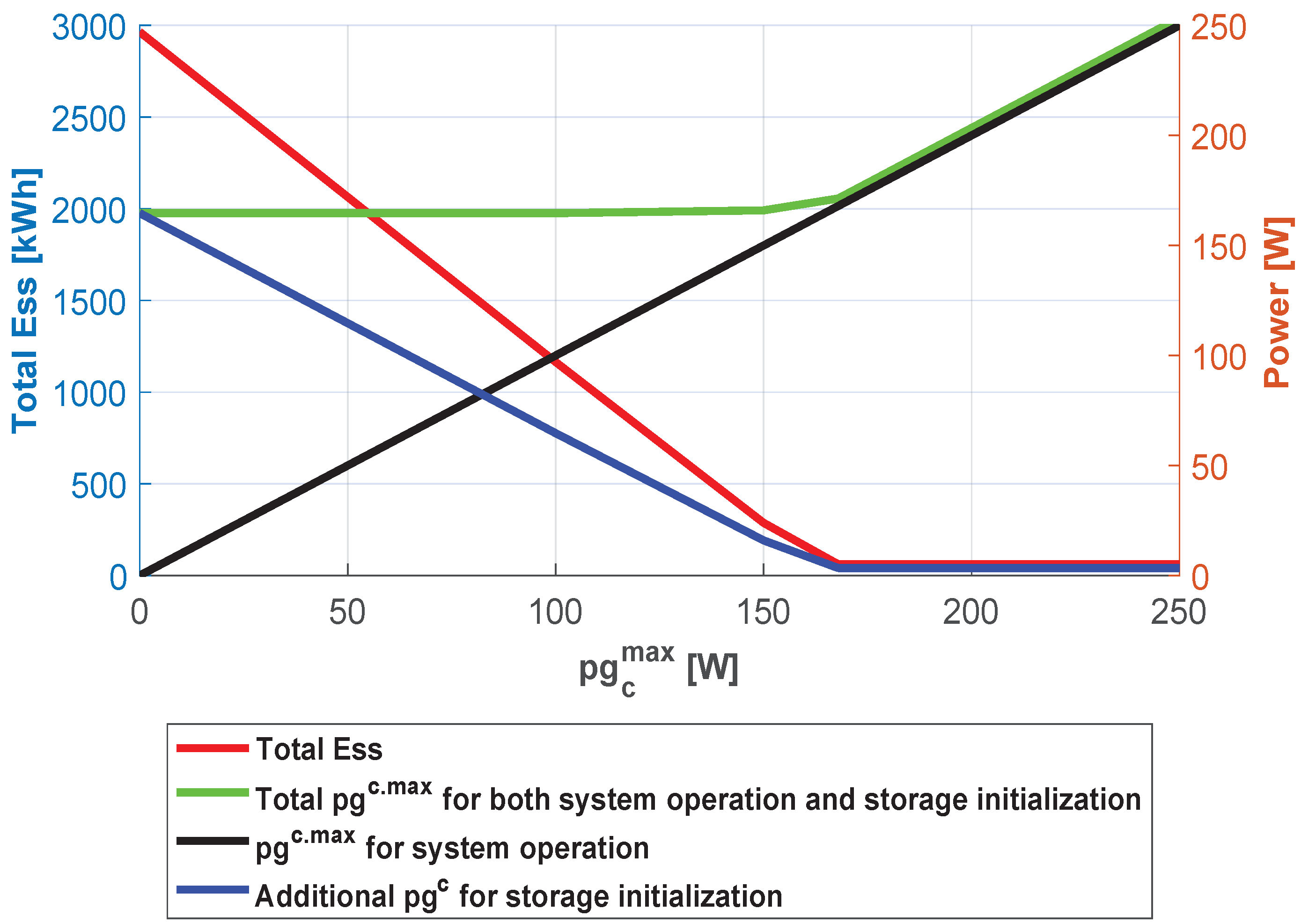
The result is shown in
Table 1 and
Figure 20 (the case of
) and
Figure 21 (the case of
). Note that each row in
Table 1 (and the set of crossing points of curves and imaginary vertical straight line) shows a possible installation (sizes) of storage devices and the maximum power needed to be taken from the grid, which guarantees safe operation of the system. From
Table 1 and
Figure 20 and
Figure 21, we can observe a clear trade-off between the total size of
of storage devices and the maximum power from the grid. A practical selection from these candidate designs considering various costs inherent to the grid and storage devices is beyond the scope of this paper.
7. Concluding Remarks
Power supply–demand balancing in power systems is an essential problem to be solved so that reliable power delivery can be guaranteed to end customers. It would be more critical when a system contains uncontrollable renewable energy sources. In this particular paper, the power flow assignment is proposed considering fluctuating and controllable power devices, storage devices, and connections between power devices. This particular paper targets the design issues by providing the guidelines for a power system such as what should be the optimal size, placement, and capacity of a power storage system requested for a given power system. It also helps to identify the physical limitation of power generators and loads that a given power system must have to continue safe operation in the presence of power fluctuations. An optimum capacity method for determining of the storage device is proposed in this paper. The installation of a storage device with a renewable energy source is used to mitigate the power fluctuations of generated power. Due to their fast response capacity and smart control, it is advisable to use storage devices in combination with renewable energy sources. However, due to the high investment costs of the storage devices, it is required to determine the suitable size of the storage capacity to fit the given system. The demonstration section shows the validation and application of the proposed characterization system conditions, which include the minimization of storage capacity using the Linear Programming (LP) framework and a balancing between storage devices and the energy from a grid in the environment of local area renewable energy sources.


