Article

Finite Control Set Model-Free Predictive Current Control of a Permanent Magnet Synchronous Motor

1
School of Mechanical Engineering, Hubei University of Automotive Technology, Shiyan 442002, China
2
Hubei Key Laboratory of Automotive Power Train and Electronic Control, Hubei University of Automotive Technology, Shiyan 442002, China
3
State Key Laboratory of Advanced Electromagnetic Engineering and Technology, School of Electrical and Electronic Engineering, Huazhong University of Science and Technology, Wuhan 430074, China
4
High-Efficiency and Energy-Saving Electrical Machine R&D Center of HUST at Zibo High-Tech Development Zone, Zibo 255039, China
*
Author to whom correspondence should be addressed.
Energies 2022, 15(3), 1045; https://doi.org/10.3390/en15031045
Submission received: 20 December 2021 / Revised: 20 January 2022 / Accepted: 24 January 2022 / Published: 30 January 2022

Abstract

:
In this paper, a finite control set model-free predictive current control (FCS-MFPCC) of a permanent magnet synchronous motor is presented. The control scheme addresses the problems of large current fluctuation and decline of the motor system performance during parameter perturbation for the traditional finite control set model predictive current control (FCS-MPCC). Firstly, the mathematical model of the motor is analyzed and derived during parameter perturbation, and a new hyperlocal model of the motor is established based on this mathematical model. Secondly, a finite control set model-free predictive current controller is designed based on the new hyperlocal model, and a current error correction factor is introduced to correct the prediction error. Meanwhile, the stability of the observer is demonstrated via the Lyapunov theory. The simulation results show that the proposed control strategy reduces current fluctuation compared with the FCS-MPCC strategy, and the system is robust during parameter perturbation.

1. Introduction

Permanent magnet synchronous motors (PMSMs) have numerous advantages, such as small size, a flexible structure, high reliability, and high power density; they have been widely adopted in many applications, e.g., aerospace, robotics, electric vehicles, etc. [1,2,3]. At present, in traditional PMSM speed control systems, a PI controller is generally used to adjust the speed; the algorithm is simple, and the parameters are easy to adjust. However, the PMSM is a complex research target; its complexity is reflected in its nonlinearity, multiple targets, strong coupling, etc. Therefore, the PI controller can only meet the control requirements within a certain range. During the running of the PMSM, when the internal parameters are perturbed and the system is disturbed on the outside, it is difficult for the PI controller to meet the application’s requirements in high-performance occasions [4,5].
Vector control technology has produced a classic control scheme, which is widely used in the electric drive industry. According to whether or not it is desirable to decouple, the vector control technology can be further divided into field-oriented control (FOC) [6], direct torque control (DTC) [7,8], etc. Over the years, motor systems have required fast current response and small fluctuation for PMSMs in high-precision, high-performance control problems; therefore, many scholars have carried out research at home and abroad, and various advanced control methods have been applied to the field of motor control, e.g., model predictive control (MPC) [9,10,11], sliding mode control [12,13], fuzzy control [14,15], neural network control [16,17], etc. MPC has attracted the attention of many scholars due to its fast response speed and its ability to achieve multiple nonlinear objectives; this has become a hot topic in the field of motor control.
MPC is divided into finite control set MPC (FCS-MPC) and continuous control set MPC (CCS-MPC) [18,19]. FCS-MPC mainly uses the discrete switch state of electronic devices, and predicts the next-moment state of the motor by the state at the current moment, based on the mathematical model of the motor. A reasonable cost function is designed, and the cost function is used to compare each predicted state quantity. The principle of minimum value is to select the optimal voltage vector and apply it to the inverter. In the actual digital control system, there is a fundamental problem of one-beat delay because of the calculation time of the algorithm and other factors. As a solution to the problem of one-beat delay, many scholars have proposed deadbeat control [20,21]. The authors of [20] proposed a robustness MPCC strategy based on predictive error compensation for the robustness of the system. In this strategy, the error between the real value of the current and the predicted value of the current is used as feedback to the current prediction. At the same time, the current errors corresponding to each voltage are obtained in a given period, ensuring the accuracy of error feedback and reducing current fluctuation. The authors of [21] proposed a static error elimination algorithm that superimposes the d-axis voltage on the d-axis current static difference integral value, and the controller’s flux linkage value is adjusted by the q-axis current’s static difference integral value in order to eliminate current fluctuations. The author of [22] proposed a method of error feedback compensation based on the application of vector prediction to further improve deadbeat control. The authors of [23] proposed a fast online current loop tuning method to solve the problem of accurate current control. In [24], current ripples of a surface-mounted PMSM were effectively reduced by applying two voltage vectors during the control period, instead of one voltage vector, as in conventional MPCC. The authors of [25] proposed a two-step CCS-MPCC strategy that was adopted to complete the PMSM mathematical model; the predictive currents could be obtained without the estimated rotor position, and a new proportional cost function was designed to obtain the optimal voltage vector.
MPC depends heavily on mathematical modeling, while model-free control is produced in theories that do not rely on mathematical models of the system. French scholar M. Fliess summarized model-free control, and proposed a PID intelligent algorithm based on a hyperlocal model on the basis of model-free control [26]. The authors of [27,28] proposed a new type of hyperlocal model in the classic model-free predictive control, which divides the parameter-unknown part into a linear part and a nonlinear part; at the same time, an extended sliding mode observer is used to solve the parameter-unknown part. The authors of [29] used the method of differential algebra to estimate the unknown part of the parameters; this method has non-incremental features, and cannot be analyzed via classical stability theory. The authors of [30,31] estimated the unknown part of the parameters in model-free control based on the extended observers of the arctangent function and the fal function, respectively, to improve system robustness. The authors of [32] proposed a compensated scheme with an extended sliding mode observer. The authors of [33] proposed a robust nonlinear predictive current control method for PMSM drives, which can optimize the current control loop performance of the PMSM system via PMSM parameter perturbation. The authors of [34,35] used different methods to solve the problem of robustness of the control system; ref. [34] proposed a method based on a hyperlocal model to solve the problem, the unknown part of which was estimated using an active disturbance rejection control algorithm; meanwhile, ref. [35] proposed an improved MPCC algorithm based on the incremental model for surface-mounted PMSM drives.
Therefore, for the traditional FCS-MPCC strategy, the performance of the motor system is reduced and the current fluctuation is large because of parameter perturbation. This paper combines model-free control with deadbeat model predictive current control, and proposes an FCS-MFPCC strategy; this control strategy does not need to know the exact mathematical model of the motor, and it can achieve good control effects under the conditions of motor parameter perturbation. Firstly, it analyzes the PMSM in detail in the event of parameter perturbation, the mathematical model of the PMSM is deduced, and a new hyperlocal model is established. Secondly, a discrete sliding mode observer is designed to accurately estimate the unknown part of the new hyperlocal model. Finally, the effectiveness of the algorithm is verified by simulation and, compared with the traditional FCS-MPCC, the current fluctuation and torque fluctuation are significantly reduced.

2. PMSM System Model Description

2.1. Mathematical Model of Permanent Magnet Synchronous Motor

Assuming that the PMSM is running in an ideal state, the permanent magnet delay phenomenon, eddy current loss, magnetic circuit, and stator core saturation are ignored; the magnetic circuit is considered to be linear, and factors such as perturbation of the motor parameters are not considered. Thus, the voltage equation of the PMSM on the dq-axis can be obtained [36]:
{ u d = R s o i d + L d o d i d d t ω r e L q o i q u q = R s o i q + L q o d i q d t ω r e L d o i d + ω r e ψ f
where, ud and uq represent the stator voltages of the dq-axis, respectively, Rso is the nominal value of the stator resistance, Ldo and Lqo are the nominal values of the stator dq axis inductance, respectively, id and iq represent the stator current of the dq-axis, respectively, ωre represents the rotor electrical angular speed, and Ψf represents the nominal value of the permanent magnet flux linkage.
When the motor is in actual operation, it is influenced by the saturation of the magnetic circuit and the electronic core, which will cause the motor resistance, inductance, and flux linkage to be perturbed. Therefore, in order to make sure that the motor maintains high performance during operation, the PMSM model under parameter perturbation can be given as follows:
{ u d = R s o i d + L d o d i d d t ω r e L q o i q + Δ u d u q = R s o i q + L q o d i q d t ω r e L d o i d + ω r e ψ f + Δ u q
where Δ u d and Δ u q represent the voltage disturbances when the motor parameters are perturbed; Δ u d and Δ u q can be expressed as follows:
{ Δ u d = Δ R s o i d + Δ L d o d i d d t ω r e Δ L q o i q Δ u q = Δ R s o i q + Δ L q o d i q d t ω r e Δ L d o i d + ω r e Δ ψ f
where Δ R s o , Δ L d o , and Δ L q o are the perturbation of the motor parameters R s o , L d o , and L q o , respectively, and Δ ψ f is the disturbance of the permanent magnet flux linkage when the flux linkage ψ f changes.
When Formula (3) is substituted into Formula (2), the state current equation of the dq-axis of the PMSM can be listed as follows:
{ d i d d t = u d L d o + Δ L d o R s o + Δ R so L d o + Δ L d o i d + ω r e L q o + Δ L q o L d o + Δ L d o i q d i q d t = u q L q o + Δ L q o R s o + Δ R so L q o + Δ L q o i q + ω r e L d o + Δ L d o L q o + Δ L q o i d + ω r e ψ f + Δ ψ f L q o + Δ L q o
When transforming Formula (4), the state current equation of the dq-axis of the motor under the perturbation of parameters is:
{ d i d d t = u d L d o R s o L d o i d + ω r e L q o + Δ L q o L d o + Δ L d o i q Δ L d o L d o ( L d o + Δ L d o ) u d Δ R s L d Δ R s L d L d o ( L d o + Δ L d o ) i d d i q d t = u q L q o R s o L q o i q u q L q o + Δ L q o + ω r e L d o + Δ L d o L q o + Δ L q o i d + ω r e Δ ψ f L q o + Δ L q o Δ L q o L q o ( L q o + Δ L q o ) u q Δ R s L q Δ R s L q L q o ( L q o + Δ L q o ) i q
The electromagnetic torque equation of the PMSM in the dq-axis is as follows:
T e = 3 2 n p [ ψ f + ( L d o L q o ) i d ] i q
The mechanical motion equation of the PMSM in the dq-axis can be expressed as follows:
d ω e d t = n p J ( T e T L B m ω r e ) ,
where T e represents the electromagnetic torque of the motor, T L represents the mechanical load torque applied, J represents the rotor inertia, Bm is the nominal value of the damping coefficient, and n p is the number of motor poles.

2.2. PMSM Hyperlocal Model

The single-input single-output nonlinear control system for the traditional hyperlocal model can be expressed as follows:
{ x ˙ = g ( x ) + α u y = x
where x represents the state variable of the system, α is the non-physical constant gain, α u and x ˙ are kept at the same order of magnitude, g ( x ) is the known part of the system and the uncertain part of the parameters., and y and u are the output and input of the system, respectively.
According to the theory of the new hyperlocal model, g ( x ) in Equation (8) can be decomposed into a linear part and a nonlinear part, so the new hyperlocal model is given as follows:
{ x ˙ = α u + β x + F y = x
where β represents the system state gain, and F represents the unknown nonlinear part, which satisfies Lipschitz boundedness and Lebesgue measurability.
According to Equations (5) and (9), the PMSM model can be expressed as follows:
{ d i d d t = α d i d + β d u d + F d d i q d t = α q i q + β q u q + F q
where α d = R s o L d o ; α q = R s o L q o ; β d = = 1 L d o ; β q = 1 L q o ; F d , F q are the unknown parts of the system.

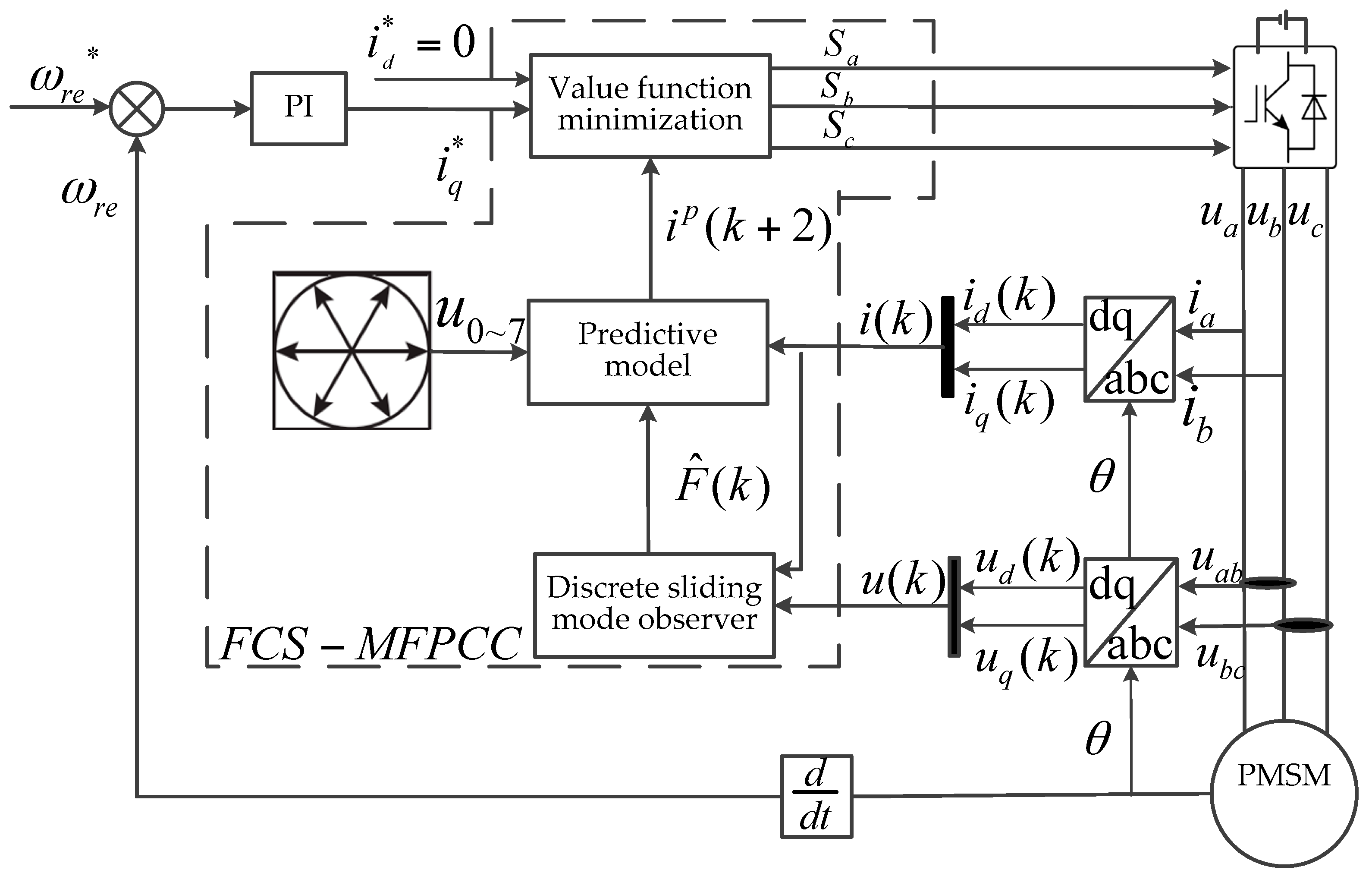
3. PMSM Model-Free Predictive Current Control

3.1. Model-Free Deadbeat Prediction Current Control Algorithm

In the traditional FCS-MPCC method, the motor mathematical model is used to predict the future value of the current. When the motor parameters are perturbed, if the model is used to predict the future value of the current, there will be deviation between the ideal model and the actual model, and the motor performance will be decreased. Therefore, this paper combines the traditional FCS-MPCC and the hyperlocal model in the model-free PCC, and the FCS-MPCC algorithm is proposed.
Discretization of Equation (10) by the forward Euler method is given as follows:
{ i d P ( k + 1 ) = ( α d i d ( k ) + β u d ( k ) + F d ( k ) ) T s + i d ( k ) i q P ( k + 1 ) = ( α q i q ( k ) + β u q ( k ) + F q ( k ) ) T s + i q ( k )
where i d P ( k + 1 ) and i q P ( k + 1 ) are the predicted current values of the dq-axis at the next sampling time, Ts is the sampling time period, and F d ( k ) and F q ( k ) represent updates in real time in each sampling period—including the unknown part—due to perturbation of the motor parameters.
The current control objective used in this paper is that the current of the motor dq-axis can follow its given reference value, as well as the difference between the stator current of the dq-axis and the reference value. The sum of the absolute values is a cost function. The cost function of Equation (12) is as follows:
J = | i q i q p ( k + 1 ) | + | i d i d p ( k + 1 ) |
where J represents the cost function, i q represents the reference stator current of the q-axis, and i d represents the reference stator current of the d-axis.
In a given sampling time period, there are eight switch states to choose from, including two zero vectors and six effective vectors. Under the action of the i-th (i = 0,1,2...7) voltage vector, combined with voltage reconstruction, the dq-axis current value at the next moment is predicted by the value function.
In theoretical research, i ( k + 1 ) can accurately track the reference value i ( k ) in a sampling period; however, in the actual running of the motor system, the motor current actually lags behind the change in the motor current. The schematic diagram of one-beat delay is shown in Figure 1. The state variable of the motor x k is obtained at the moment t k ; the time at this point is t 1 , and after the filter delay time in the digital system, the optimal voltage vector will be chosen at the moment t 2 , or it will have an effect on the motor at t 3 , and the state of the motor will change from x k to x k + 1 , but in the ideal state, the optimal voltage vector should be applied to the motor at t k , and will cause one-beat delay.
In order to solve the problem of one-beat delay, this article adopts the delay compensation method based on the two-step operation to compensate for the system delay. Specifically, the state parameters at time k are substituted into Equation (11), the current value is predicted at time k + 1, and the current value is obtained at time k + 2 using Equation (13). The corresponding current expression can be given as follows:
{ i d P ( k + 2 ) = ( α d i d η ( k + 1 ) + β u d ( k + 1 ) + F d ( k ) ) T s + i d η ( k + 1 ) i q P ( k + 2 ) = ( α q i q η ( k + 1 ) + β u q ( k + 1 ) + F q ( k ) ) T s + i q η ( k + 1 )
where i d P ( k + 2 ) and i q P ( k + 2 ) represent the current prediction value of the dq-axis at ( k + 2 ) T s , while i d η ( k + 1 ) and i q η ( k + 1 ) represent the estimated values of the actual current of the dq-axis at time k + 1 , respectively. Calculating the predicted current value i d P ( k + 1 ) , i q P ( k + 1 ) at time k + 1 by Formula (11), i d P ( k + 1 ) and i q P ( k + 1 ) are used instead of i d η ( k + 1 ) and i q η ( k + 1 ) . Therefore the predicted current value after two-step prediction can be expressed as follows:
{ i d P ( k + 2 ) = ( α d i d p ( k + 1 ) + β d u d ( k + 1 ) + F d ( k + 1 ) ) T s + i d p ( k + 1 ) i q P ( k + 2 ) = ( α q i q p ( k + 1 ) + β q u q ( k + 1 ) + F q ( k + 1 ) ) T s + i q p ( k + 1 )
It should be noted that the predicted current value at k + 2 represents the predicted current value calculated in the first step, and the first and second steps use the same voltage vector. When the sampling period Ts is very small, it can be considered that F d ( k + 1 ) = F d ( k ) , F q ( k + 1 ) = F q ( k ) .

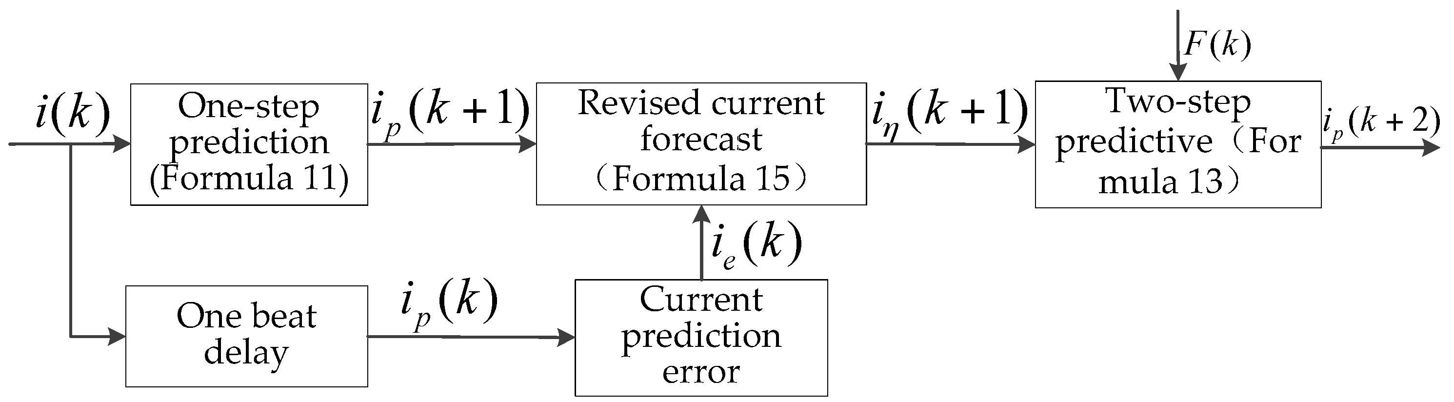
3.2. Predicted Current Error Feedback Compensation

If i d p ( k + 1 ) = i d η ( k + 1 ) and i q p ( k + 1 ) = i q η ( k + 1 ) are used directly in Formula (14), it will cause the system to generate a larger prediction error. Thereby, the accuracy of current tracking is reduced, and the predicted current correction links are introduced to correct the predicted current, as follows:
{ i d η ( k + 1 ) = i d p ( k + 1 ) + k 1 Δ i d ( k ) i q η ( k + 1 ) = i q p ( k + 1 ) + k 2 Δ i q ( k )
where Δ i d ( k ) and Δ i q ( k ) are the respective current difference values generated when each voltage is applied to the motor at t k , and the expressions are Δ i d ( k ) = i d p ( k ) i ( k ) , Δ i q ( k ) = i q p ( k ) i ( k ) , and k 1 , k 2 are the difference coefficients of the dq-axis, respectively. Figure 2 shows an improved deadbeat current prediction control diagram.
Through deadbeat current predictive control, the corresponding value function expression can be written as follows:
J = | i q i q p ( k + 2 ) | + | i d i d p ( k + 2 ) |

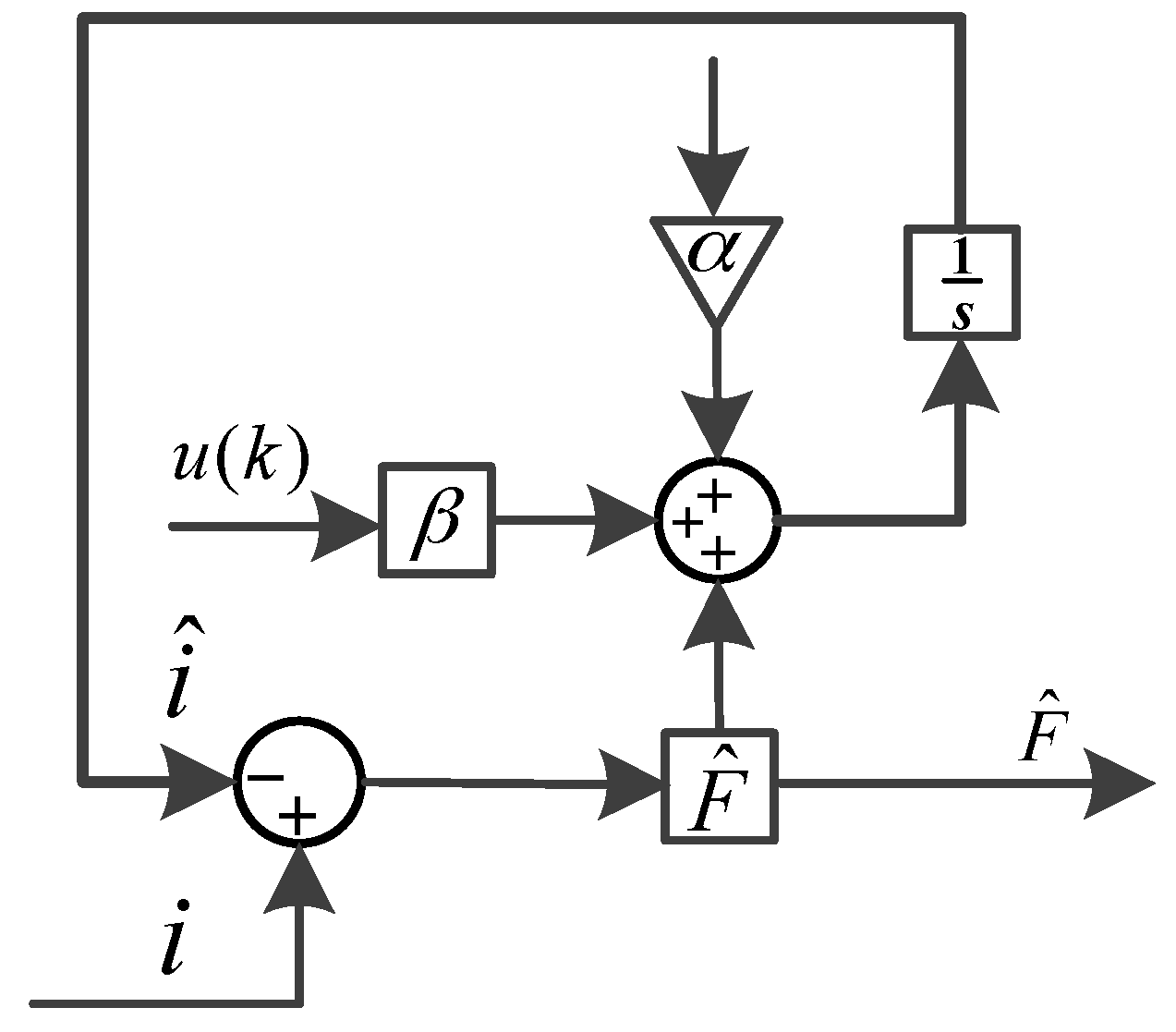
4. Design of the Extended Sliding Mode Observer

4.1. Design of the Sliding Mode Observer

The accurate estimation of F plays a vital role in the control performance of the system. In this paper, the following sliding mode observer is used to estimate the value of F [30]:
i ^ ˙ = α i ^ + β u + γ | i i ^ | δ sgn ( i i ^ ) + k ( i i ^ )
where k is the coefficient of the exponential term; k > 0 , δ is the exponent of the power term; δ = σ + ( λ σ ) e ξ | x | ; x is the state variable, and x = i i ^ is taken as the state variable below; lim t | x | = 0 , λ and σ are the δ parameter can reach the minimum and maximum values; 0 < λ < 1 , σ > 0 , ξ is the coefficient of the constant term that adjusts the rate of change of δ ; ξ > 0 , γ = d i a g ( γ 1 , γ 2 ) , γ 1 > 0 , γ 2 > 0 are the parameters to be designed; i ^ ˙ represents the observed values of i ^ , i ^ = [ i ^ d i ^ q ] T ; sgn ( ) is the symbolic function; and u = [ u d u q ] T , i = [ i d i q ] T .
The observer error is defined as follows:
e = i i ^
where e = [ e d e q ] T , e d = i d i ^ d , e q = i q i ^ q .
Through Equations (10) and (17), the observer error equation can be written as follows:
e ˙ = α e + F γ | e | σ + ( λ σ ) e ξ | e | sgn ( e ) k e
This paper selects the sliding mode surface s = e and selects the appropriate matrix γ . It can be proven that the observer error equation can converge to zero by Equation (19).
Proof: choose the following Lyapunov function to prove the stability of Equation (17):
V = 1 2 s 2
The derivative of Equation (20) is taken, then Equation (19) is substituted, and it can be obtained through the following calculations:
V = s s ˙ = s ( α s + F γ | s | σ + ( λ σ ) e ξ | e | sgn ( s ) k s ) = s α s + s F s γ | s | σ + ( λ σ ) e ξ | e | sgn ( s ) s k s s α s + s F γ s | s | σ + ( λ σ ) e ξ | e | s k s s ( α s + F γ | s | σ + ( λ σ ) e ξ | e | )
where · represents the matrix norm or the vector norm; although s and F are unknown, they are considered to be bounded in the actual application process. Therefore, if γ α s + F | s | σ + ( λ σ ) e ξ | e | + η , η > 0 , it can be determined from Equation (21) that:
V ˙ η e < 0
According to the stability judgment of the Lyapunov function and the reachable condition of the sliding mode, the error e will gradually converge to zero in a finite time. Therefore, the sliding mode observer Equation (17) designed in this paper is asymptotically stable.

4.2. Discretization of Sliding Mode Observer

In the actual digital control system, the sliding mode observer designed in this paper needs to run in a discrete digital control system. Therefore, the designed sliding mode observer must be discretized. For small T s 1 , Equation (17) can be discretized as follows:
i ^ ( k + 1 ) = ( α + I ) i ^ ( k ) + β u ( k ) + γ | e ( k ) | σ + ( λ σ ) e ξ | e | sgn ( e ( k ) ) k e ( k )
where i ^ ( k + 1 ) refers to the current observation value at time (k + 1)Ts, i ^ ( k ) is the current observation value at time kTs, i ^ ( k + 1 ) = [ i ^ d ( k + 1 ) i ^ q ( k + 1 ) ] , i ^ ( k ) = [ i ^ d ( k ) i ^ q ( k ) ] , u ( k ) is the voltage value at time kTs, u ( k ) = [ u d ( k ) u q ( k ) ] , e ( k ) is the current error variation at time k, e ( k ) = [ e d ( k ) e q ( k ) ] , and I is the identity matrix.
According to the principle of sliding mode equivalence e ˙ = e = 0 , the unknown quantity F can be obtained from Equation (19).
F ^ ( k ) = γ | e ( k ) | α + ( λ α ) e β | e ( k ) | sgn ( e ( k ) ) + k e ( k )
In order to effectively reduce the vibration caused by the sign function of the sliding mode observer, the arctangent function is used instead of the sign function. Equation (24) can be rewritten as Equation (25). Figure 3 shows a block diagram for solving unknown quantity F .
F ^ ( k ) = γ | e ( k ) | α + ( λ α ) e β | e ( k ) | arctan ( e ( k ) ) + k e ( k )
In summary, the block diagram of the FCS-MPFCC strategy is shown in Figure 4. The specific steps are as follows:
  • According to Equations (17) and (18), the current error variable e ( k ) is solved at time k ;
  • The unknown quantity F is observed through the sliding mode observer (Equation (25));
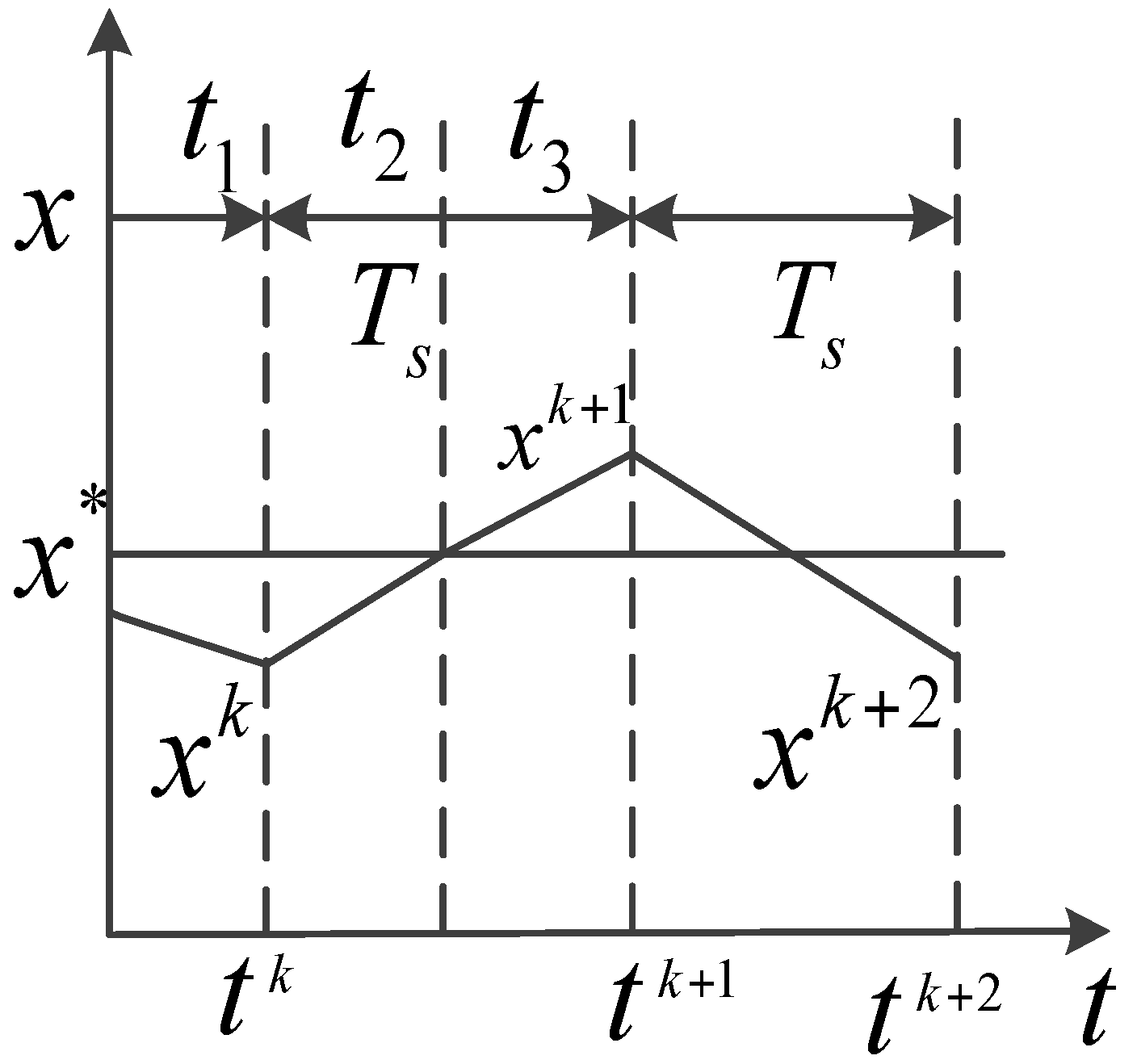
  • The current value of the present period is predicted through the voltage value and actual current value at time k 1 ;
  • The predicted current value is corrected according to Equation (15) to obtain i d η ( k + 1 ) , i q η ( k + 1 ) ;
  • The observed F is substituted into Equations (11) and (13) to obtain the predicted current values i d p ( k + 2 ) and i q p ( k + 2 ) at time k + 2 ;
  • According to the principle of the minimum value of the value function, the optimal voltage vector corresponding to the minimum value of Equation (16) is selected to be used in the inverter.
Figure 4. Block diagram of FCS-MPFCC.
Energies 15 01045 g004

5. Simulation Results and Discussion

In order to verify the feasibility and effectiveness of FCS-MFPCC, the simulation was carried out in MATLAB/Simulink, and the traditional FCS-MPCC simulation model was simulated under the same conditions.
Table 1 shows the nominal parameters of the PMSM. The control strategy of i d = 0 was adopted in the simulation. The speed rating was 300 r/min, the current rating was 10 A, and the torque rating was 10 N.m. The sampling period was set to 10 us or 50 us, and the PI parameters were k p = 2 , k i = 20 ; in model-free control, the values of α d , α q , β d , and β q are determined by α d = R s o L d , α q = R s o L q , β d = = 1 L d o , and β q = 1 L q o , respectively. The parameters of the sliding mode observer are σ = 1.5 , λ = ξ = 0.5 , γ = 15 , k = 10 . In the current error correction, k 1 = k 2 = 0.92 .

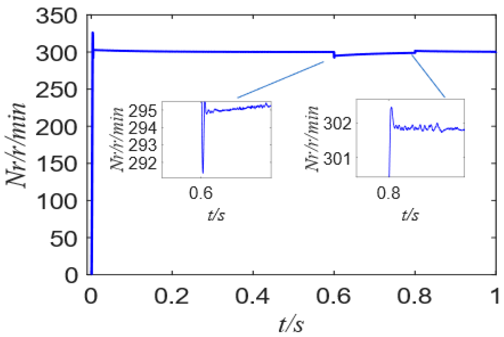
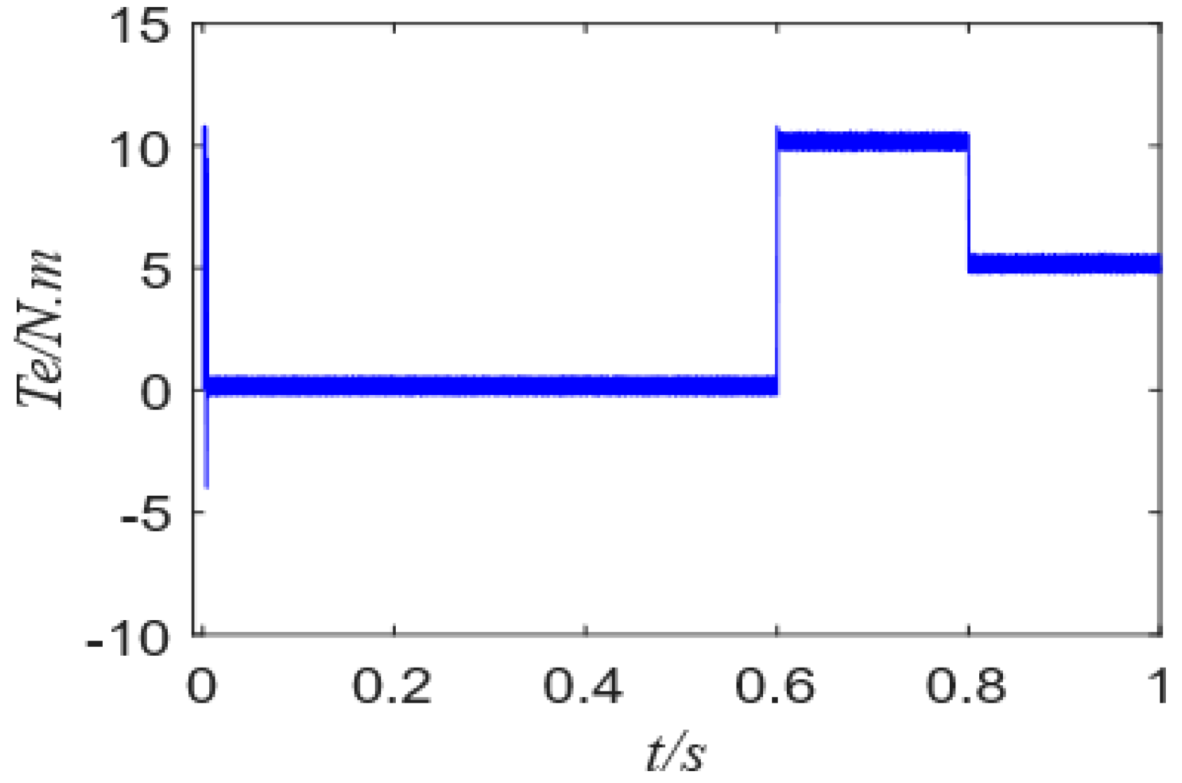
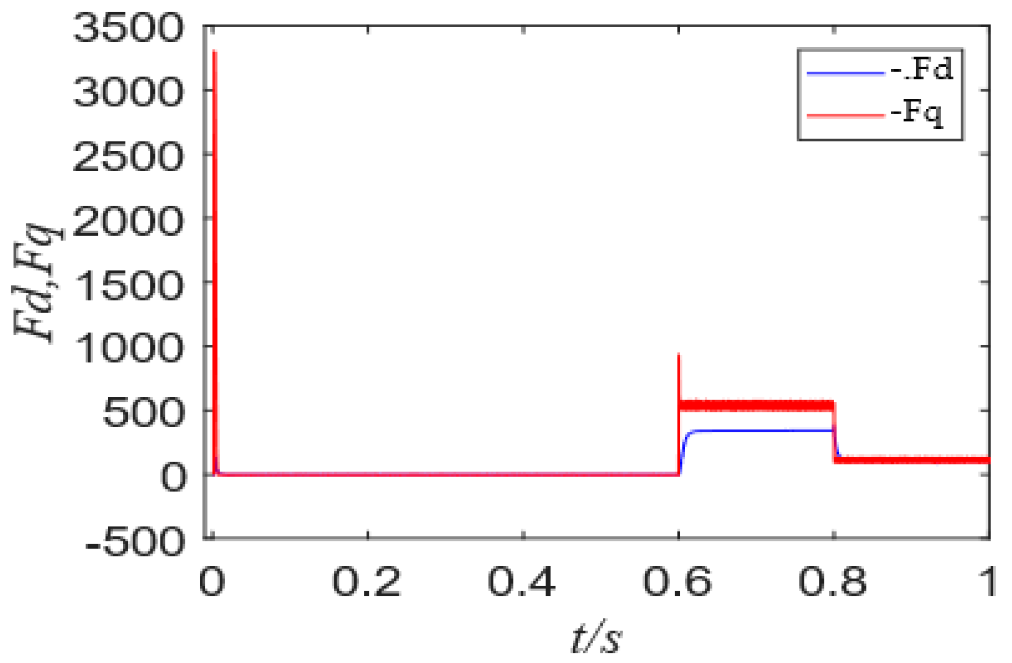
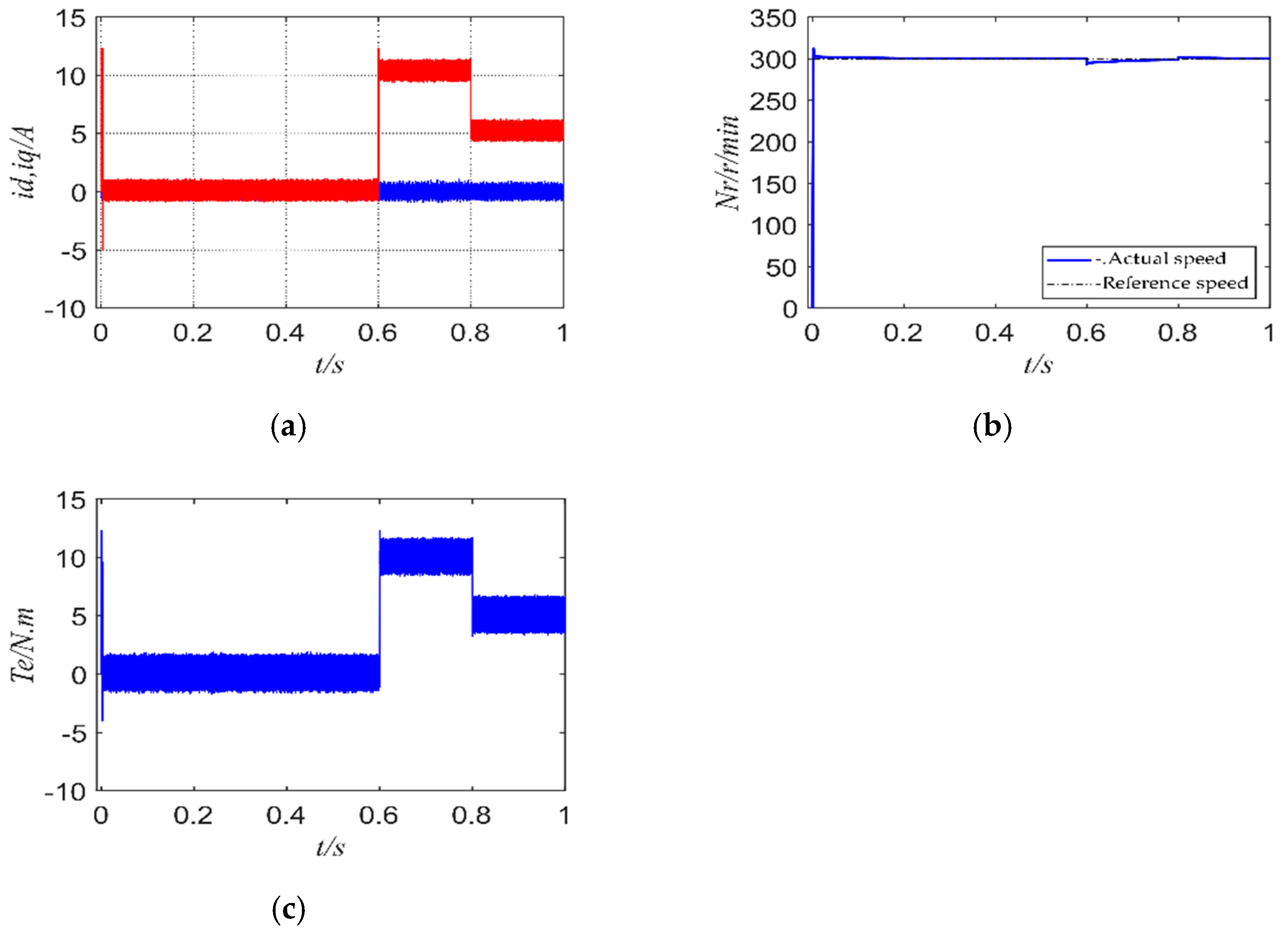
5.1. Simulation Results and Discussion of PMSM under Normal Parameters

In the simulation conditions, the reference speed was 300 r/min, the motor is no-load when starting, the load torque was increased to 10 N·m at 0.6 s, and the load torque changed to 5 N·m at 0.8 s. The motor parameters were all nominal values.
Figure 5 and Figure 6 show the d-axis current of FCS-MPCC and FCS-MPFCC, Figure 7 and Figure 8 show the q-axis current of FCS-MPCC and FCS-MPFCC. It can be seen in Figure 5 and Figure 6 that the d-axis current fluctuation has decreased. Although FCS-MFPCC has a certain overshoot when the motor starts, it is still smaller than the fluctuation of FCS-MPCC. Comparing Figure 7 with Figure 8, it can be clearly seen that the current fluctuation of the q-axis has decreased significantly. At the same time, in the case of 0.6 s and 0.8 s torque mutation, the overshoot is also significantly reduced, and the response can quickly reach the corresponding reference value.
Figure 9 and Figure 10 show the rotation speed waveform of the FCS-MPCC and FCS-MPFCC; Figure 11 and Figure 12 show the torque waveform of the FCS-MPCC and FCS-MFPCC, while Figure 13 shows the waveforms of FCS-MFPCC unknown quantities Fd and Fq. Comparing Figure 9 and Figure 10, it can clearly be seen that the speed response is similar and can reach the reference value quickly, but under the control of FCS-MFPCC, the overshoot is changed from 316 r/min to 326 r/min when the motor starts, and the overshoot increases by 10 r/min, but the overshoot changes from 291.2 r/min to 292.3 r/min in 0.6 s, becoming smaller, and when the torque changes at t = 0.8 s, the overshoot changes from 302.7 r/min to 301.9 r/min. As can be seen from Table 2, the speed fluctuation of FCS-MFPCC is smaller, and the fluctuation of FCS-MPCC in 0~0.6 s is greater than that of FCS-MFPCC, which is caused by the larger overshoot when the motor starts. Comparing Figure 11 with Figure 12, it can be seen that the torque ripple is reduced, the overshoot is reduced, and the response speed is similar. It can be seen from Figure 13 that the unknown quantities Fd and Fq change at 0.6 s and 0.8 s, respectively, providing an accurate prediction for the observer.
Figure 14 shows the simulation results of FCS-MFPCC when the sampling period is 50 us. It can be seen from Figure 14 that the simulation still maintains good results.
Through analysis, it can be seen that the FCS-MFPCC algorithm affords improvements over the FCS-MPCC algorithm; not only does it not affect the dynamic performance when the motor parameters are unchanged, but its dynamic performance is improved. The fast response characteristic of the traditional algorithm is maintained.
Table 2 shows the quantitative comparison results of the FCS-MPCC algorithm when the sampling period is 10 us, along with the quantitative comparison results of the FCS-MFPCC algorithm when the sampling period is 10 us and 50 us, including qd-axis current ripple, average torque, and speed ripple, as calculated by Equation (26).
σ = ( x i μ ) 2 N
where σ is the average pulsation, μ is the average value of the sampled data, x i is the sampled value, and N is the number of adopted data.

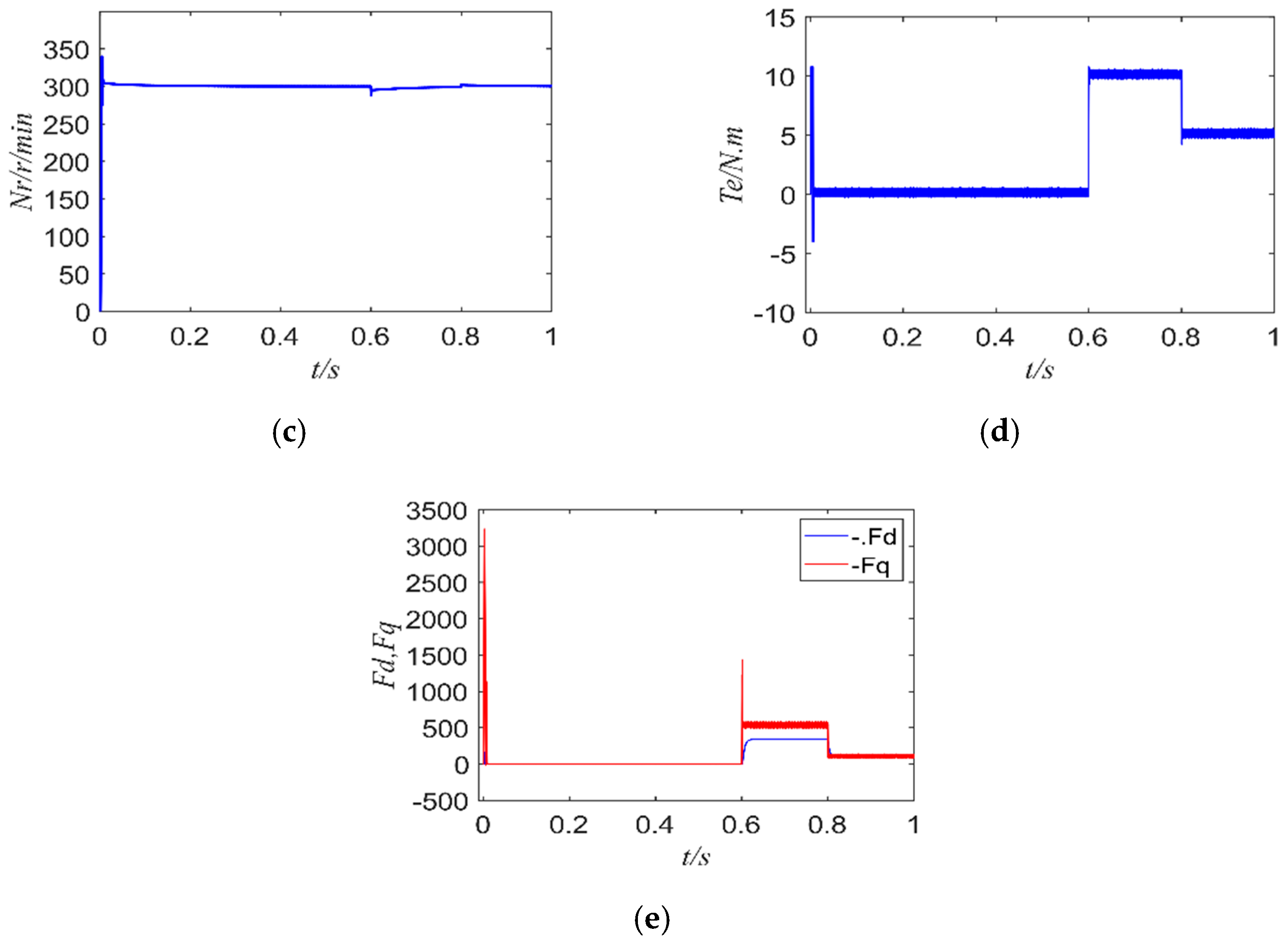
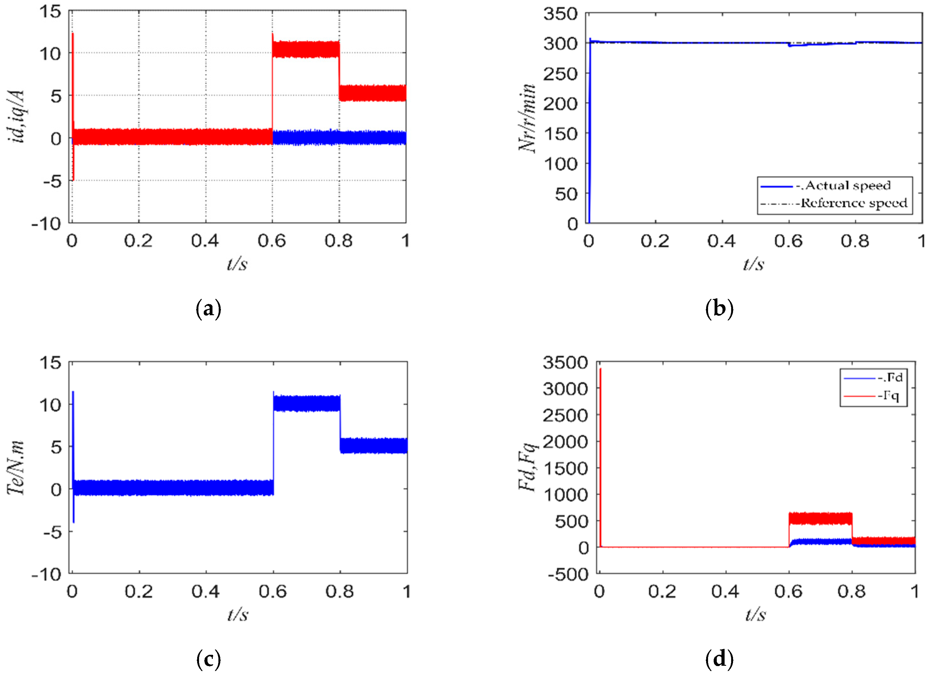
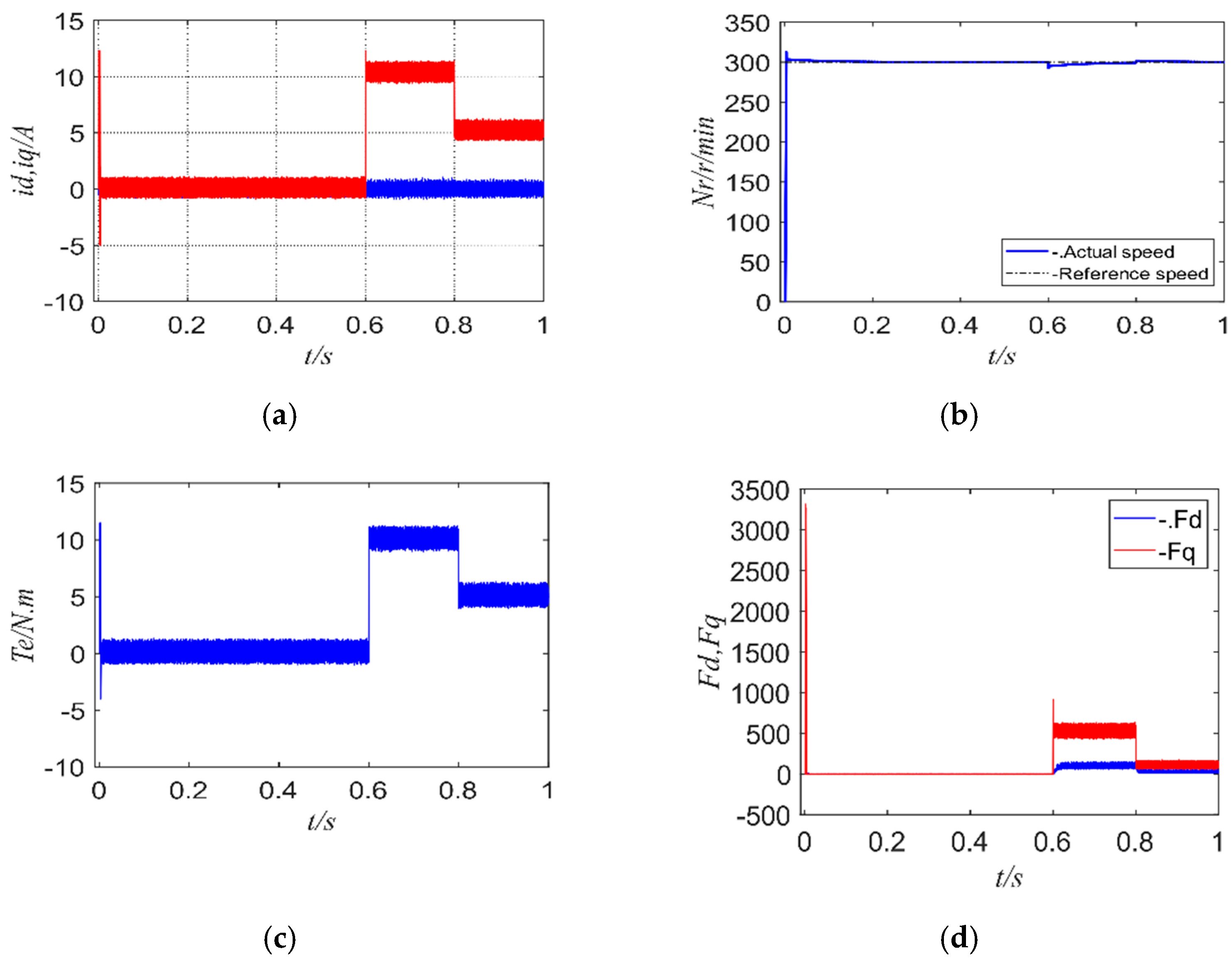
5.2. Simulation Results and Discussion of PMSM under Parameter Perturbation

The control performance of the FCS-MPCC algorithm and the FCS-MFPCC algorithm was compared when the motor parameters were perturbed. The simulation conditions were set as follows: the reference speed was 300 r/min, the motor was no-load when starting, the load torque was increased to 10 N·m in 0.6 s, and the load torque was suddenly changed to 5 N·m in 0.8 s. Rs = 0.738 Ω; Ld = Lq = 0.0012 Mh; other motor parameters were nominal values.
Figure 15 and Figure 16 show the simulation results of the two control methods in the event of parameter perturbation. Figure 15a and Figure 16a show the dq-axis current waveforms of the two control methods; Figure 15b and Figure 16b show the motor speed waveforms of the two control methods; Figure 15c and Figure 16c show the torque waveforms of the two control methods; Figure 16d shows the waveform of the unknown quantities Fd and Fq.
Comparing Figure 15 with Figure 16, it can be seen that in the event of motor parameter perturbation, the dq-axis current of the FCS-MPCC algorithm fluctuates greatly, and the load torque also fluctuates greatly, causing unstable speed, and the actual speed deviates from the reference speed. FCS-MFPCC also shows better control performance. Compared with FCS-MFPCC, the traditional FCS-MPCC has a larger overshoot of q-axis current and torque, indicating that the proposed FCS-MFPCC algorithm is more robust than FCS-MPCC. From Figure 16d, it can be seen that FCS-MFPCC shows high performance, and the unknown quantities Fd and Fq are accurately estimated as being closely related.
Figure 17 shows the simulation results of FCS-MFPCC under parameter perturbation when the sampling period is 50 us. It can be seen from Figure 17 that the simulation results of the sampling periods of 10 us and 50 us are similar, both of which can maintain good steady-state performance and robustness.
Through the analysis above, it can be determined that the control performance of the traditional FCS-MPCC is more affected when the motor is perturbed by resistance and inductance; under the same simulation conditions, the steady-state error of the dq-axis current and torque becomes worse, as does the response. This proves that once some unknown disturbances occur, the FCS-MPCC control method cannot guarantee that the motor can maintain a high performance.
Table 3 shows the quantitative comparison results of the FCS-MPCC algorithm when the sampling period is 10 us, and the quantitative comparison results of the FCS-MFPCC algorithm when the sampling period is 10 us and 50 us under parameter perturbation, including qd-axis current ripple, average torque, and speed ripple, as calculated by Equation (26).

6. Conclusions

There are always a large current ripple and parameter perturbation problems that cause the mismatch between the prediction model and the actual model during the operation of the motor. To overcome this problem, an effective FCS-MFPCC algorithm is proposed. This algorithm combines model-free control, deadbeat control, and the FCS-MPCC algorithm, and then the finite control set model-free predictive current controller is designed on the basis of the new hyperlocal model. The deadbeat two-step current predictive control method with predictive current error correction is applied to the current inner loop, the accuracy and stability of the system are improved, and a new reaching-law-based sliding mode control algorithm is used to precisely estimate the unknown part of the new hyperlocal model, and the stability of the sliding mode observer is demonstrated using the Lyapunov theory. Compared with the traditional FCS-MPCC algorithm, the simulation results show that the FCS-MFPCC algorithm can reduce the steady-state error of the current, and it also has better transient performance and greater robustness when the motor parameters are perturbed. Quantitatively, the improvements this makes to the MPCC include reducing the current fluctuation by 51.01%, 53.96%, and 55.61% and the torque fluctuation by 0.9%, 32.30%, and 39.39% in 0–0.6 s, 0.6–0.8 s, and 0.8–1 s, respectively, when the motor parameters are the nominal values. In addition, the FCS-MFPCC algorithm not only retains the fast response characteristic of the traditional FCS-MPCC algorithm, but also decreases the dependence of the motor on the mathematical model.

Author Contributions

The FCS-MFPCC algorithm was suggested and designed by F.Y., M.H. and Y.L. The writing of the original draft was carried out by F.Y. Writing, reviewing, and editing were carried out by M.H., Y.L., F.Y. and L.W. All authors have read and agreed to the published version of the manuscript.

Funding

For this work, no external funding was received.

Acknowledgments

This work was supported by Key R&D Projects in Hubei Province: 2020BAA005; the Industrial Internet Innovation and Development Project of the Ministry of Industry and Information Technology: TC200802C, TC200A00W; the Outstanding Youth Fund Project of Shandong Provincial Natural Science Foundation: ZR2020YQ40; and the Ministry of Education’s Coordinates Education Project: 201802240009.

Conflicts of Interest

The authors declare no conflict of interest.

References

  1. Ismagilov, F.; Vavilov, V.; Gusakov, D.; Uzhegov, N. Topology Selection of the High-speed High-voltage PMSM for Aerospace Application. In Proceedings of the IECON 2017—43RD Annual Conference of the IEEE Industrial Electronics Society, Beijing, China, 29 October–1 November 2017; Volume 10, pp. 2219–2224. [Google Scholar]
  2. Yuan, G.G.; Guo, R.S.; Sun, J.Y. The Application of PMSM in Motor Drive Control System of patrol Robot. Int. J. Control Automation. 2016, 9, 303–308. [Google Scholar] [CrossRef]
  3. Li, X.Q.; Meng, D.Z.; Yang, J.Q. Research on Decoupling Technology of Permanent Magnet Synchronous Motor Braking Current of Electric Vehicle Based on Identity Matrix. Large Electr. Mach. Hydraul. Turbine 2021, 4, 19–23+34. [Google Scholar]
  4. Zhao, K.H.; Li, P.; Zhang, C.F.; Li, X.F.; He, J.; Lin, Y.L. Sliding mode observer-based current sensor fault reconstruction and unknown load disturbance estimation for PMSM driven system (Article). Sensors 2017, 17, 2833. [Google Scholar] [CrossRef] [PubMed] [Green Version]
  5. Zhu, L.; Wen, X.H.; Zhao, F.; Kong, L. Control policies to prevent PMSMs from losing control under field-weakening operation. Proc. Chin. Soc. Electr. Eng. 2011, 31, 67–72. [Google Scholar]
  6. Li, Y.; Huang, H.B.; Cheng, S.Q.; Zhao, Y.; Wu, W.L. Design of MTPA control system for permanent magnet synchronous motor. J. Hubei Automot. Ind. Inst. 2021, 35, 65–70. [Google Scholar]
  7. Nasr, A.; Gu, C.; Bozhko, S.; Gerada, C. Performance Enhancement of Direct Torque-Controlled Permanent Magnet Synchronous Motor with a Flexible Switching Table. Energies 2020, 13, 1907. [Google Scholar] [CrossRef] [Green Version]
  8. Karlovsky, P.; Lettl, J. Induction Motor Drive Direct Torque Control and Predictive Torque Control Comparison Based on Switching Pattern Analysis. Energies 2018, 11, 1793. [Google Scholar] [CrossRef] [Green Version]
  9. Bouguenna, I.F.; Tahour, A.; Kennel, R.; Abdelrahem, M. Multiple-Vector Model Predictive Control with Fuzzy Logic for PMSM Electric Drive Systems. Energies 2021, 14, 1727. [Google Scholar] [CrossRef]
  10. Shi, J.X.; Xie, Z.X.; Chen, Z.Y.; Qiu, J.Q. Parameter-free hyperlocal model predictive control of permanent magnet synchronous motors. J. Electric Mach. Control 2021, 25, 1–8. [Google Scholar]
  11. Yang, F.; Hu, M.M.; Chen, X. Improved dual vector model predictive current control for permanent magnet synchronous motors. Mot. Control Appl. 2021, 48, 21–26. [Google Scholar]
  12. Zhang, Y.Q.; Yin, Z.G.; Li, W.; Liu, J.; Zhang, Y.P. Adaptive Sliding-Mode-Based Speed Control in Finite Control Set Model Predictive Torque Control for Induction Motors. IEEE Trans. Power Electron. 2021, 36, 8076–8087. [Google Scholar] [CrossRef]
  13. Guo, Z.H.; Zhu, J.G. Sliding mode control of six-phase permanent magnet synchronous motor based on a new approaching law. Large Electr. Mach. Hydraul. Turbine 2020, 2, 1–6. [Google Scholar]
  14. Pedapenki, K.K.; Kumar, J.; Anumeha. Fuzzy Logic Controller-Based BLDC Motor Drive. In Recent Advances in Power Electronics and Drives; Springer: Singapore, 2020; Volume 707, pp. 379–388. [Google Scholar]
  15. Jin, F.Z.; Wan, H.; Huang, Z.F.; Gu, M.X. PMSM Vector Control Based on Fuzzy PID Controller. J. Phys. Conf. Ser. 2020, 1617, 012016. [Google Scholar] [CrossRef]
  16. Yang, X.W.; Deng, W.X.; Yao, J.Y. Neural network based output feedback control for DC motors with asymptotic stability. Mech. Syst. Signal Processing 2022, 164, 108288. [Google Scholar] [CrossRef]
  17. Xu, Y.Z.; Yang, J.B.; Fang, L. Permanent magnet synchronous motor power supply imbalance and phase loss fault diagnosis based on artificial neural network. Large Electr. Mach. Hydraul. Turbine 2016, 4, 1–5+9. [Google Scholar]
  18. Zhong, Z.Z. Research on Predictive Current Control of Permanent Magnet Synchronous Motor with Finite Set Model; Guangdong University of Technology: Guangdong, China, 2020. [Google Scholar]
  19. Bao, G.Q.; Qi, W.G.; He, T. Direct Torque Control of PMSM with Modified Finite Set Model Predictive Control. Energies 2020, 13, 234. [Google Scholar] [CrossRef] [Green Version]
  20. Yao, X.L.; Ma, C.W.; Wang, J.F.; Huang, C.Q. Robust permanent magnet synchronous motor model predictive current control based on prediction error compensation. Proc. Chin. Soc. Electr. Eng. 2021, 41, 6071–6081. [Google Scholar]
  21. Liu, J.Q.; Hao, W.J.; Chen, A.F.; Tian, J.H. Research on deadbeat predictive current control strategy of permanent magnet synchronous motors. J. China Railw. Soc. 2021, 43, 62–72. [Google Scholar]
  22. He, C. Permanent Magnet Synchronous Motor Model Predictive Current Control Based on Finite Control Set; Harbin Institute of Technology: Harbin, China, 2019. [Google Scholar]
  23. You, Z.C.; Huang, C.H.; Yang, S.M. Online Current Loop Tuning for Permanent Magnet Synchronous Servo Motor Drives with Deadbeat Current Control. Energies 2019, 12, 3555. [Google Scholar] [CrossRef] [Green Version]
  24. Bozorgi, A.M.; Farasat, M.; Jafarishiadeh, S. Model predictive current control of surfacemounted permanent magnet synchronous motor with low torque and current ripple. IET Power Electron. 2017, 10, 1120–1128. [Google Scholar] [CrossRef]
  25. Luo, X.; Shen, A.; Tang, Q.P.; Liu, J.C.; Xu, J.B. Two-Step Continuous-Control Set Model Predictive Current Control Strategy for SPMSM Sensorless Drives. In Proceedings of the IEEE Transactions on Energy Conversion, Trieste, Italy, 5 August 2020; pp. 1110–1120. [Google Scholar]
  26. Fliess, M.; Join, C. Model-free control. Int. J. Control 2013, 86, 2228–2252. [Google Scholar] [CrossRef] [Green Version]
  27. Zhao, K.H.; Dai, W.K.; Zhou, R.R.; Leng, A.J.; Liu, W.C.; Qiu, P.Q.; Huang, G.; Wu, G.P. New model-free sliding mode control of permanent magnet synchronous motor based on extended sliding mode disturbance observer. Proc. Chin. Soc. Electr. Eng. 2021, 59, 1–13. Available online: http://kns.cnki.net/kcms/detail/11.2107.TM.20210824.1016.002.html (accessed on 27 November 2021).
  28. Zhao, K.H.; Zhou, R.R.; Leng, A.J.; Dai, W.K.; Huang, G. A finite set model-free fault-tolerant predictive control algorithm for permanent magnet synchronous motors. Trans. China Electrotech. Soc. 2021, 36, 27–38. [Google Scholar]
  29. Su, G.J.; Li, H.M.; Li, Z.; Zhou, Y.N. Model-free current control of permanent magnet synchronous linear motors. Trans. China Electrotech. Soc. 2021, 36, 3182–3190. [Google Scholar]
  30. Wang, Y.Q.; Zhu, Y.C.; Feng, Y.T.; Tian, B. A new approaching law sliding mode control strategy for permanent magnet synchronous motors. Electr. Power Autom. Equip. 2021, 41, 192–198. [Google Scholar]
  31. Hou, L.M.; He, P.Y.; Wang, W.; Yan, X.; Tu, N.W. Research on PMSM model-free adaptive sliding mode control based on ESO. Control Eng. China 2021, 28, 1–8. [Google Scholar]
  32. Shao, M.; Deng, Y.; Li, H.; Liu, J.; Fei, Q. Sliding Mode Observer-Based Parameter Identification and Disturbance Compensation for Optimizing the Mode Predictive Control of PMSM. Energies 2019, 12, 1857. [Google Scholar] [CrossRef] [Green Version]
  33. Lyu, M.; Wu, G.; Luo, D.; Rong, F.; Huang, S. Robust Nonlinear Predictive Current Control Techniques for PMSM. Energies 2019, 12, 443. [Google Scholar] [CrossRef] [Green Version]
  34. Zhang, Y.C.; Jin, J.L.; Huang, L.L. Model-Free Predictive Current Control of PMSM Drives Based on Extended State Observer Using Ultralocal Model. IEEE Trans. Ind. Electron. 2021, 68, 993–1003. [Google Scholar] [CrossRef]
  35. Zhang, X.G.; Zhang, L.; Zhang, Y.C. Model Predictive Current Control for PMSM Drives with Parameter Robustness Improvement. IEEE Trans. Power Electron. 2019, 34, 1645–1657. [Google Scholar] [CrossRef]
  36. Yuan, L.; Hu, B.X.; Wei, K.Y.; Chen, S. Modern Permanent Magnet Synchronous Motor Control Principle and Matlab Simulation; Beijing University of Aeronautics and Astronautics Press: Beijing, China, 2016. [Google Scholar]
Figure 1. Schematic diagram of one-beat delay.
Energies 15 01045 g001
Figure 2. Block diagram of improved deadbeat current prediction control.
Energies 15 01045 g002
Figure 3. Block diagram of solving unknown quantity F ^ .
Energies 15 01045 g003
Figure 5. d-axis current of FCS-MPCC.
Energies 15 01045 g005
Figure 6. d-axis current of FCS-MFPCC.
Energies 15 01045 g006
Figure 7. q-axis current of FCS-MPCC.
Energies 15 01045 g007
Figure 8. q-axis current of FCS-FMPCC.
Energies 15 01045 g008
Figure 9. Rotation speed of FCS-MPCC.
Energies 15 01045 g009
Figure 10. Rotation speed of FCS-MFPCC.
Energies 15 01045 g010
Figure 11. Torque of FCS-MPCC.
Energies 15 01045 g011
Figure 12. Torque of FCS-MFPCC.
Energies 15 01045 g012
Figure 13. Observed values of unknown quantities Fd and Fq.
Energies 15 01045 g013
Figure 14. FCS-MPCC simulation results under normal parameters when the sampling period is 50 us: (a) dq-axis current of FCS-MPCC; (b) speed of FCS-MPCC; (c) torque of FCS-MPCC; (d) torque of FCS-MFPCC; (e) observed values of unknown quantities Fd and Fq.
Energies 15 01045 g014aEnergies 15 01045 g014b
Figure 15. FCS-MPCC simulation results under parameter perturbation: (a) dq-axis current of FCS-MPCC; (b) speed of FCS-MPCC; (c) torque of FCS-MPCC.
Energies 15 01045 g015
Figure 16. FCS-MFPCC simulation results under parameter perturbation when the sampling period is 10 us: (a) dq-axis current of FCS-MFPCC; (b) speed of FCS-MFPCC; (c) torque of FCS-MFPCC; (d) observed values of the unknown quantities Fd and Fq under parameter perturbation.
Energies 15 01045 g016
Figure 17. FCS-MFPCC simulation results under parameter perturbation when the sampling period is 50 us: (a) dq-axis current of FCS-MFPCC; (b) speed of FCS-MFPCC; (c) torque of FCS-MFPCC; (d) observed values of the unknown quantities Fd and Fq under parameter perturbation.
Energies 15 01045 g017
Table 1. Nominal parameters of PMSM.
ParametersNumerical Value
Flux induced by magnets Ψf/Wb0.129
Stator inductance Ls/mH2.4
d-axis inductance Ld/mH2.4
q-axis inductance Lq/mH2.4
Motor stator resistance Rs/Ω0.369
Number of poles np5
Rotor inertia J/kgm20.001916
Damping coefficient Bm/Nm·rad/s0.00464
Table 2. Errors of different control methods.
ParametersTs (us)Error (Standard Deviation)
No Load (0 s~0.6 s)Load (0.6 s~0.8 s)Load (0.8 s~1 s)
id (A)FCS-MPCC100.26190.27260.2848
FCS-MFPCC100.12830.12550.1264
FCS-MFPCC500.14710.14580.1442
iq (A)FCS-MPCC100.85210.43870.3135
FCS-MFPCC100.81110.29700.1900
FCS-MFPCC500.90540.38270.1921
Te (N·m)FCS-MPCC100.79540.42440.3033
FCS-MFPCC100.74430.28740.1838
FCS-MFPCC500.83020.37030.1859
Nr (r/min)FCS-MPCC1011.43571.14300.3226
FCS-MFPCC1012.48561.14080.3188
FCS-MFPCC5013.51781.31760.4598
Table 3. Errors of different control methods under parameter perturbation.
ParametersTs (s)Error (Standard Deviation)
No Load (0 s~0.6 s)Load (0.6 s~0.8 s)Load (0.8 s~1 s)
id (A)FCS-MPCC100.72880.73040.7218
FCS-MFPCC100.44650.44710.4373
FCS-MFPCC50 0.29640.32080.3215
iq (A)FCS-MPCC101.05830.75360.7332
FCS-MFPCC100.86220.44740.4299
FCS-MFPCC500.85580.42890.3552
Te (N·m)FCS-MPCC101.02730.72910.7094
FCS-MFPCC100.81260.43280.4160
FCS-MFPCC500.80440.41500.3437
Nr (r/min)FCS-MPCC1010.92081.25630.4608
FCS-MFPCC1011.54661.24910.4588
FCS-MFPCC5012.16401.25790.4589
Publisher’s Note: MDPI stays neutral with regard to jurisdictional claims in published maps and institutional affiliations.

